| Issue |
A&A
Volume 571, November 2014
|
|
|---|---|---|
| Article Number | A51 | |
| Number of page(s) | 18 | |
| Section | Planets and planetary systems | |
| DOI | https://doi.org/10.1051/0004-6361/201322090 | |
| Published online | 06 November 2014 | |
Near-infrared emission from sublimating dust in collisionally active debris disks⋆
1
Astronomical Institute “Anton Pannekoek”, University of
Amsterdam,
PO Box 94249,
1090 GE
Amsterdam,
The Netherlands
e-mail:
This email address is being protected from spambots. You need JavaScript enabled to view it.
2
Department of Astrophysics/IMAPP, Radboud University
Nijmegen, PO Box
9010, 6500 GL
Nijmegen, The
Netherlands
3
Leiden Observatory, Leiden University,
PO Box 9513, 2300 RA
Leiden, The
Netherlands
Received: 14 June 2013
Accepted: 8 April 2014
Abstract
Context. Hot exozodiacal dust is thought to be responsible for excess near-infrared (NIR) emission emanating from the innermost parts of some debris disks. The origin of this dust, however, is still a matter of debate.
Aims. We test whether hot exozodiacal dust can be supplied from an exterior parent belt by Poynting–Robertson (P–R) drag, paying special attention to the pile-up of dust that occurs owing to the interplay of P–R drag and dust sublimation. Specifically, we investigate whether pile-ups still occur when collisions are taken into account, and if they can explain the observed NIR excess.
Methods. We computed the steady-state distribution of dust in the inner disk by solving the continuity equation. First, we derived an analytical solution under a number of simplifying assumptions. Second, we developed a numerical debris disk model that for the first time treats the complex interaction of collisions, P–R drag, and sublimation in a self-consistent way. From the resulting dust distributions, we generated thermal emission spectra and compare these to observed excess NIR fluxes.
Results. We confirm that P–R drag always supplies a small amount of dust to the sublimation zone, but find that a fully consistent treatment yields a maximum amount of dust that is about 7 times lower than that given by analytical estimates. The NIR excess due to this material is much less (≲10-3 for A-type stars with parent belts at ≳1 AU) than the values derived from interferometric observations (~10-2). Pile-up of dust still occurs when collisions are considered, but its effect on the NIR flux is insignificant. Finally, the cross-section in the innermost regions is clearly dominated by barely bound grains.
Key words: zodiacal dust / circumstellar matter
Appendices are available in electronic form at http://www.aanda.org
© ESO, 2014
1. Introduction
Circumstellar dust in debris disks reveals the location and dynamical state of larger bodies and thus sheds light on the architecture of planetary systems in the aftermath of planet formation (see Wyatt 2008 for a review). The dust can be studied by observing its infrared and (sub-)millimeter emission, as well as the stellar radiation it scatters, and is usually found at large distances from the star (tens of AUs, Carpenter et al. 2009). Recently, interferometric observations have found excess near-infrared (NIR) emission emanating from the innermost parts of several debris disks, which has been interpreted as thermal emission from hot (>1000 K) dust (Ciardi et al. 2001; Absil et al. 2006, 2008, 2009; di Folco et al. 2007; Akeson et al. 2009; Defrère et al. 2011, 2012, see Table 1 for an overview). This material is known as hot exozodiacal dust. Its origin, hence what it can tell us about planet formation, is still unclear. In this work, we investigate one possible scenario for explaining hot exozodiacal dust.
NIR interferometric detections of hot exozodiacal dust, together with associated outer debris belt locations.
Dust grains in debris disks have relatively short lifetimes because of their destruction by collisions and removal by radiation forces. To detect these grains around mature stars therefore implies the existence of a mechanism that continuously replenishes them. Cold dust populations at large distances from the star can be maintained by a collisional cascade grinding down much larger bodies that act as a reservoir of mass (Backman & Paresce 1993). Closer to the star, however, the pace at which material is processed by collisions is much higher, so that the lifetime of a debris belt in collisional equilibrium is much shorter there (Dominik & Decin 2003; Wyatt et al. 2007). For this reason, hot exozodiacal dust cannot be explained by in situ planetesimal belts (Wyatt et al. 2007; Lebreton et al. 2013)1, and a different mechanism is needed to replenish it, the lifetime of the dust needs to be extended by some process, or both.
Many of the systems that exhibit NIR excess also feature a debris belt at a large distance from the star (see Table 1). Inward transport of material from an outer belt may therefore be a natural explanation for the existence of hot exozodiacal dust. A possible transportation mechanism is Poynting–Robertson (P–R) drag (see, e.g., Burns et al. 1979). Because P–R drag acts on a timescale that is much longer than that of collisions, it is sometimes not favored as a possible mechanism for maintaining exozodiacal dust (e.g., Absil et al. 2006). However, as long as there are no mechanisms that prevent inward migration, a small amount of dust is always transported to the innermost part of the disk (Wyatt 2005), where it produces a NIR signal.
Morphological models of exozodiacal dust disks, constrained by the NIR observations, indicate that the hot dust is concentrated in a sharply peaked ring, whose inner boundary is determined by dust sublimation (Defrère et al. 2011; Mennesson et al. 2013; Lebreton et al. 2013). The process of dust sublimation may therefore play an important role in shaping exozodiacal clouds. Kobayashi et al. (2009) find that the interplay between P–R drag and dust sublimation can lead to a local enhancement of dust in the sublimation zone, leading to radial distributions of dust reminiscent of those found by the morphological models. However, they only investigate this pile-up effect for drag-dominated systems, where collisions are unimportant, and it is unclear what happens to the phenomenon if collisions are taken into account.
In this work, we examine whether it is possible to maintain a pile-up of dust in the sublimation zone of a collisionally active debris disk and whether such a pile-up could explain the exozodiacal NIR emission observed very close to some stars. To do this, we compute the steady-state distribution of dust in the inner parts of debris disks by solving the continuity equation, considering collisions, P–R drag, and sublimation. First, we find an analytical solution, using a number of simplifying assumptions (Sect. 2). Subsequently, we solve the continuity equation numerically using a debris disk model that for the first time treats the complex interaction of collisions, P–R drag, and sublimation in a self-consistent way (Sect. 3). From the obtained steady-state dust distributions, we compute emission spectra to compare with observational data (Sect. 4). We discuss our findings in Sect. 5, and give conclusions in Sect. 6. Details of the numerical techniques employed by the debris disk model are given in Appendix A, model verification tests are described in Appendix B, and the post-processing of model output into useful physical quantities in described in Appendix C.
2. Analytical constraints
In this section we analytically investigate the distribution of dust in the inner regions of debris disks. We focus on the radial distribution of material, by assuming (1) that the disk is axisymmetric and (2) that all particles have the same size. Throughout this work, radial distributions are expressed in terms of vertical geometrical optical depth, which is defined as the surface density of cross-section2. Under the two assumptions listed above, it is given by  (1)Here, r is the radial distance from the central star, σ the cross-section of a particle, and n(r) the one-dimensional number density (i.e., the particle number density integrated over disk height and azimuth).
We consider three processes affecting the evolution of dust particles in debris disks: collisions, P–R drag, and sublimation. The strategy for our analytical estimates is as follows. First, we review the balance between P–R drag and collisions (without considering sublimation) and calculate the inward flux of material due to these two effects (Sect. 2.1). Subsequently, we consider the interplay of P–R drag and sublimation (ignoring collisions), which can lead to the pile-up of dust in the sublimation zone (Sect. 2.2). Finally, we investigate whether collisions can be neglected in the innermost parts of a debris disk and estimate the radial distribution of dust in a disk where all three processes are in operation (Sect. 2.3). At the end of the section, we briefly summarize our findings (Sect. 2.4).
2.1. Poynting–Robertson drag and collisions
The balance between P–R drag and collisions was studied analytically by Wyatt (2005). Because of its importance to the present study, we summarize the main arguments of this work here. The model assumes that (1) there is a source of dust at distance r0 with a geometrical optical depth of τgeo(r0); (2) dust particles follow circular orbits; (3) collisions are always destructive; and (4) all dust grains have the same size. These assumptions lead to simple expressions for the timescales on which P–R drag and collisions typically act.
The P–R drag timescale tPR is defined as the time it takes for a particle on a circular orbit to spiral from a given distance r to the central star. It is given by (e.g., Burns et al. 1979)  (2)where c is the speed of light, G the gravitational constant, M⋆ the stellar mass, and β the ratio of the norms of the direct radiation pressure force and the gravitational force on a particle (β = | Frp/Fg |)3.
The collisional timescale tcoll indicates the average time between two collisions for a given particle. Wyatt (2005) finds  (3)where torb is the orbital period of a circular orbit, given by
  . This equation is valid for particles that are on circular orbits and whose most important collisional partners have similar sizes4.
2.1.1. The radial distribution due to P–R drag and collisions
Under the assumptions listed above, there is an analytical solution to the continuity equation, balancing the migration of particles due to P–R drag with the destruction of dust by collisions. Wyatt (2005) finds that the steady-state solution is 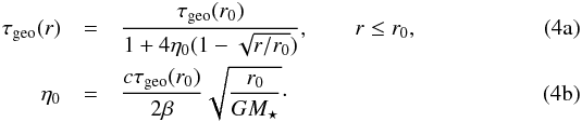 The parameter η0 characterizes the density of the parent belt. It is defined such that for η0 = 1 the collisional and P–R drag timescales are equal at r0. Disks with η0> 1 are collision-dominated at r0, while disks with η0< 1 are drag-dominated at r0. Most debris disks with observed outer belts have η0> 10 (Wyatt 2005).
The balance between P–R drag and collisions is self-limiting: a denser parent belt produces more dust drifting inwards, but this dust also suffers more mutual collisions that eliminate grains on their way in. This results in a maximum geometrical optical depth profile for η0 ≫ 1 (i.e., a very dense parent belt) of ![Mathematical equation: \begin{equation} \label{eq:max_tau_eff} \max[\tau\sub{geo}(r)] = \frac{ \sqrt{ G M\sub{\star} } \, \beta }{ 2 c \left( \sqrt{ r\sub{0} } - \sqrt{ r } \right) }, \qquad r \leq r\sub{0}. \end{equation}](/articles/aa/full_html/2014/11/aa22090-13/aa22090-13-eq44.png) (5)Figure 1 shows examples of this radial profile for different parent belt locations and host star masses, all for dust grains with β = 0.5. The value for β was set to the blowout limit: particles with β> 0.5 leave the system on hyperbolic paths after they are released from a large parent body on a circular orbit. Therefore, P–R drag is the most efficient for β = 0.5, and for a given system, this value corresponds to the maximum τgeo profile5.
(5)Figure 1 shows examples of this radial profile for different parent belt locations and host star masses, all for dust grains with β = 0.5. The value for β was set to the blowout limit: particles with β> 0.5 leave the system on hyperbolic paths after they are released from a large parent body on a circular orbit. Therefore, P–R drag is the most efficient for β = 0.5, and for a given system, this value corresponds to the maximum τgeo profile5.
 |
Fig. 1 Maximum geometrical optical depth as a function of distance to the star (Eq. (5)). The profiles are derived from the analytical model of Wyatt (2005), in which dust is produced by a source at radius r0 and subsequently migrates inward due to P–R drag, while suffering destruction from mutual collisions. The solid lines correspond to solar-mass stars, the dashed lines to 2 M⊙ stars. Profiles for different parent belt locations are shown in different colors. All profiles assume dust grains with β = 0.5. |
2.1.2. The inward flux of material
Since dust can pile up close to the star due to sublimation (to be discussed in Sect. 2.2.2), τgeo may exceed the upper limit given by Eq. (5) in the sublimation zone. The material that piles up, however, is supplied from farther out by P–R drag. To investigate the properties of the pile-up, it is therefore useful to assess the inward flux of material.
In the case of a uniform grain size, the inward particle flux due to P–R drag (i.e., the number of particles passing through a ring at radius r per unit of time) can be expressed as  (6)where ṙPR is the P–R drag velocity, counted positively towards r> 0. If the particle orbits are circular, radial migration due to P–R drag is described by (e.g., Burns et al. 1979)
  (7)The grain parameter β can be expressed as (e.g., Burns et al. 1979)
  (8)Here, L⋆ is the stellar luminosity, m the mass of an individual dust grain, and Qpr the radiation pressure efficiency averaged over the stellar spectrum. Combining Eqs. (1), (6)–(8) and multiplying by particle mass m gives the inward (collision-limited) P–R drag mass flux (cf. Rafikov 2011)
  (9)The maximum mass flux can now be found by substituting Eq. (5) for τgeo(r) in Eq. (9), which yields
 ![Mathematical equation: \begin{equation} \label{eq:max_mass_flux} \max \left[ \dot{ M }\sub{PR}(r) \right] = \frac{ \sqrt{ G M\sub{\star} } \, L\sub{\star} \beta Q\sub{pr} } { 2 c^3 \left( \sqrt{ r\sub{0} } - \sqrt{ r } \right) }, \qquad r \leq r\sub{0}. \end{equation}](/articles/aa/full_html/2014/11/aa22090-13/aa22090-13-eq60.png) (10)Figure 1 shows that max [ τgeo(r) ] levels off in the innermost part of the system (r ≪ r0), at the radii where exozodiacal dust is seen. The mass flux corresponding to this plateau is
(10)Figure 1 shows that max [ τgeo(r) ] levels off in the innermost part of the system (r ≪ r0), at the radii where exozodiacal dust is seen. The mass flux corresponding to this plateau is ![Mathematical equation: \begin{eqnarray} \label{eq:max_mass_flux_r0} \max [ \dot{ M }\sub{PR}( r = 0 ) ] && \approx 5.6 \times 10^{-13} \, \biggl( \frac{ M\sub{\star} }{ \mathrm{1~M}\sub{\odot} } \biggr)^{1/2} \, \biggl( \frac{ L\sub{\star} }{ \mathrm{1~L}\sub{\odot} } \biggr) \nonumber \\ && \quad \times \biggl( \frac{ r\sub{0} }{ \mathrm{1~AU} } \biggr)^{-1/2} \, \biggl( \frac{ Q\sub{pr} }{ 1 } \biggr) \, \biggl( \frac{ \beta }{ 0.5 } \biggr) \; {M}\sub{\earth} \; \mathrm{yr}^{-1}. \end{eqnarray}](/articles/aa/full_html/2014/11/aa22090-13/aa22090-13-eq63.png) (11)The maximum mass flux only depends on grain properties through Qpr and β6. The radiation pressure efficiency Qpr must obey 0 ≤ Qpr ≤ 2, and particles with β> 1 are always unbound. Therefore, Eq. (11) with Qpr = 2 and β = 1 gives a solid upper limit on the inward mass flux due to P–R drag, unless one of the model assumptions does not hold (e.g., collisions are non-destructive).
(11)The maximum mass flux only depends on grain properties through Qpr and β6. The radiation pressure efficiency Qpr must obey 0 ≤ Qpr ≤ 2, and particles with β> 1 are always unbound. Therefore, Eq. (11) with Qpr = 2 and β = 1 gives a solid upper limit on the inward mass flux due to P–R drag, unless one of the model assumptions does not hold (e.g., collisions are non-destructive).
2.2. P–R drag and sublimation
In the preceding, we found that P–R drag supplies a small but non-zero amount of dust to the innermost parts of a debris disk. As this material approaches the central star, it is heated by stellar radiation. Eventually, the dust grains become so hot that they start sublimating. We now review the evolution of these particles considering P–R drag and sublimation, but ignoring collisions.
2.2.1. Dust sublimation formalism
For a spherical dust grain in a gas-free environment, the rate at which the grain radius s changes is given by (e.g., Kobayashi et al. 2008)  (12)Here, Pv is the phase-equilibrium vapor pressure, ρd the bulk density of the dust, μ the molecular weight of dust molecules, mu the atomic mass unit, kB the Boltzmann constant, and T the temperature of the dust. This theoretical sublimation rate is sometimes lowered to comply with experimental results, parameterized in a sticking efficiency or accommodation coefficient. Here, we ignore this weak effect, by assuming a sticking efficiency of unity.
The temperature dependence of Pv is given by (Kobayashi et al. 2009)  (13)where P0 is a normalization constant and H the latent heat of sublimation. By assuming P0 is constant, we neglect a small temperature dependence beyond the exponential.
Sublimation parameters depend on material and can be determined by laboratory measurements. The material we consider in this study is carbonaceous dust. This choice is motivated by the proximity of hot exozodiacal dust to its host star, which suggests a very refractory material, like carbon (Mennesson et al. 2013; Lebreton et al. 2013). Specifically, we use the sublimation parameters of graphite, for which many laboratory measurements are available. For the molecular weight, we use μ = 36.03, reflecting that graphite sublimation typically releases clusters of three carbon atoms at the temperatures and pressures relevant to this work (Abrahamson 1974). The parameters for C3 sublimation are P0 = 2.95 × 10¹⁴ dyn cm-2 and H = 2.15 × 10¹¹ erg g-1 (Zavitsanos & Carlson 1973). For the bulk density of the material, we use ρd = 1.8 g cm-3.
For our analytical estimates, we approximate the grain temperature T by its black-body temperature  (14)where σSB is the Stefan–Boltzmann constant. In reality, the grain temperature is a function of size. Temperatures are generally higher than Tbb for particles that are smaller than the typical wavelength of the stellar radiation, because these grains do not cool efficiently. For simplicity, we ignore this effect here and investigate it further in our numerical calculations, which use realistic grain temperatures (see Sect. 3.2.2).
In the black-body approximation, the sublimation rate ṡ becomes independent of grain size. This leads to a simple expression for the sublimation timescale tsubl, defined as the time it takes for a spherical dust grain to disappear, which is  (15)This estimate assumes that the grain temperature remains constant (at Tbb) throughout the sublimation process. As a sublimating particle becomes smaller, the black-body approximation is bound to become inaccurate. For sufficiently large particles, however, the true sublimation time is dominated by the black-body regime, and Eq. (15) provides a good approximation.
2.2.2. The pile-up of dust in the sublimation zone
As dust grains become smaller due to sublimation, their β-ratio changes. As a result of this, the interplay between P–R drag and sublimation can lead to a pile-up of dust in the sublimation zone. This phenomenon was studied in detail by Kobayashi et al. (2008, 2009, 2011). Here, we give a brief explanation of the pile-up mechanism.
When dust grains migrate inward owing to P–R drag, their temperature gradually increases. At some point, the grains are heated to the point where sublimation becomes substantial, and their sizes start decreasing significantly. For particles larger than the peak wavelength of the stellar spectrum λ⋆7, the radiation pressure efficiency is roughly constant at Qpr ≈ 1, and therefore the approximation β ∝ s-1 holds (see Eq. (8)). As the particles lose mass, radiation pressure therefore becomes more important (relative to stellar gravity), which has the effect of increasing the semi-major axes and eccentricities of their orbits, compensating for the decrease terms due to P–R drag. This effectively slows down the inward migration of the dust grains, leading to an accumulation of dust in the sublimation zone. Eventually, the dust grains either sublimate completely or their β ratios increase to the point where they become unbound and are blown out of the system.
Accumulation of dust occurs when the decrease of semi-major axis due to P–R drag is compensated by the increase of semi-major axis due to sublimation. This happens approximately at the radial distance where the timescale of P–R drag equals that of sublimation (Kobayashi et al. 2008)8, We denote this distance with rpile, and determine its value by solving tPR(rpile) = tsubl(rpile). Assuming that the dust in the pile-up has the black-body temperature Tpile = Tbb(rpile), which holds for s ≳ λ⋆, this equation can be written as  (16)which shows that Tpile is independent of stellar parameters, the bulk density of the dust, and grain size (Qpr is nearly constant for s ≳ λ⋆), and only depends on material properties (cf. Kobayashi et al. 2008, 2009, 2011). Using Qpr = 1 and the sublimation parameters of graphite given in Sect. 2.2.1, we numerically solve Eq. (16) to find Tpile ≈ 2020 K, hence
  (17)The pile-up distance is independent of grain size because larger particles take longer to sublimate, but also migrate more slowly because of P–R drag. This holds as long as the black-body approximation is valid, so the grain temperature in the pile-up is independent of grain size.
2.2.3. Conditions for dust pile-up
Kobayashi et al. (2011) list two conditions for the accumulation of dust to be substantial: (1) sufficiently high values of β need to be reached as dust grains sublimate; and (2) the orbital eccentricities of the dust grains need to be low enough when they enter the sublimation zone.
Considering an inward stream of dust grains with a range of sizes, the particles contributing the most to the pile-up are those with the highest β. These particles have the strongest P–R drag drift rates, so per unit of time more of them arrive in the sublimation zone, where their inward drift is canceled as a result of sublimation. In addition, for the typical size distribution resulting from a collisional cascade, the total cross-section is dominated by the smallest particles. Since dust grains with β> 0.5 are typically blown out as soon as they are created, particles that are barely bound (β ≈ 0.5) before the onset of substantial sublimation are the most important for the pile-up. A requirement for dust migration to slow down is that β increases as the grain size decreases. For a given system, however, β reaches a maximum value βmax at s ~ λ⋆, because smaller particles have lower Qpr. Considering that relatively high values of β are needed for an efficient pile-up, low luminosity stars do not have significant pile-ups. Kobayashi et al. (2009, 2011) set the limit at βmax> 0.5, and derive a lower limit on the stellar luminosity for significant pile-up, assuming that Qpr ≈ 1 holds for s ≳ λ⋆. This limit is 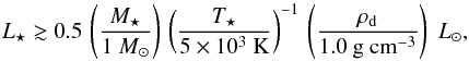 (18)where T⋆ is the effective temperature of the central star.
The pile-up of dust in the sublimation zone is highly dependent on the eccentricity of the dust as it enters the sublimation zone (Kobayashi et al. 2008). For the pile-up mechanism to produce a significant enhancement, the eccentricity of the dust particles in the sublimation zone must be very low (e ≲ 10-2; Kobayashi et al. 2008, 2011). Particles with higher orbital eccentricities do not spend enough time in the sublimation zone before they are blown out (or sublimate completely) to contribute significantly to the dust enhancement.
When dust particles are created in collisions in the parent belt, they are put on eccentric orbits with their periastron in the parent belt. Particles released from circular orbits will acquire orbital eccentricities of  (19)The particles that are the most important for the pile-up are the ones with β ≈ 0.5. These barely bound particles initially follow very elliptic orbits, with eccentricities close to unity.
The initial eccentricity of the β ≈ 0.5 particles is far too high for any significant pile-up to occur. However, as the dust grains migrate inward owing to P–R drag, their orbits are circularized. The eccentricity evolution of dust particles experiencing P–R drag is coupled to their orbital size evolution according to (Wyatt & Whipple 1950) 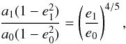 (20)where (a0,e0) are the initial semi-major axis and eccentricity, which evolve into (a1,e1). This coupling can be used to place a lower limit on the distance of the source region, if significant pile-up is to occur, using the maximum allowed eccentricity in the sublimation zone for efficient pile-up. Written in terms of periastron distance q = a(1 − e), Eq. (20) becomes
 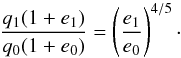 (21)Substituting r0 and rpile for q0 and q1, respectively, and using e0 ≈ 1 and e1 ≲ 10-2, yields a lower limit on the source radius
  (22)for a significant enhancement in the dust density to be possible. Other mechanisms may help in the circularization of the orbits of small particles, decreasing the limit on r0. An example is the drag force from small amounts of gas that are present in the disk (Takeuchi & Artymowicz 2001).
2.3. Pile-up in a collisionally active disk
So far, we have looked separately at the balance between P–R drag and collisions (without considering sublimation) and at the balance between P–R drag and sublimation (without considering collisions). We now investigate under what conditions this pairwise approach is justified, and combine the previous findings to estimate the distribution of dust in a debris disk in which all three processes are operational.
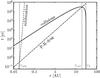 |
Fig. 2 Characteristic timescale as function of radial distance for sublimation (Eq. (15)), P–R drag (Eq. (2)), and mutual collisions (minimum timescale, Eq. (23)), for β = 0.5 particles in a debris disk around a solar-mass star with a very dense (η0 ≫ 1) parent belt located at 30 AU. The gray vertical lines indicate the radial distances used by the analytical model: rpile is the radius for which the sublimation timescale equals the P–R drag timescale, rcrit is the radius for which the P–R drag timescale equals the collisional timescale, and r0 is the location of the parent belt. For the sublimation timescale, we assume that the dust grains are solid spheres of graphite (see Sect. 2.2.1 for the values of the sublimation parameters) with a radius of s = 0.64 μm (the size corresponding to β = 0.5). |
2.3.1. Do collisions interfere with dust pile-up?
Since collisions might interfere with the process of dust pile-up, the results of Sect. 2.2 are only valid if collisions do not play an important role at distances where sublimation becomes significant. We now investigate whether collisions can indeed be neglected in the inner regions of debris disks by comparing the characteristic timescales of the three processes as a function of radius.
In the case of a very dense parent belt (η0 ≫ 1), τgeo(r) is given by Eq. (5). Putting this in Eq. (3) results in the minimum collisional timescale ![Mathematical equation: \begin{equation} \label{eq:min_t_coll} \min \left[ t\sub{coll}(r) \right] = \frac{ c r^{3/2} }{ \beta G M\sub{\star} } \left( \sqrt{ r\sub{0} } - \sqrt{ r } \right), \qquad r \leq r\sub{0}. \end{equation}](/articles/aa/full_html/2014/11/aa22090-13/aa22090-13-eq129.png) (23)In Fig. 2 this timescale is compared with the sublimation and P–R drag timescales for a debris disk around a solar-mass star with a dense parent belt at 30 AU, consisting of barely bound (β = 0.5) dust grains and using the sublimation parameters of graphite. In this example system, the collisional timescale is longer than the other timescales at rpile, implying that P–R drag dominates collisions in the sublimation zone, and collisions do not interfere with dust pile-up. We now check whether this a general result or under which conditions it is the case.
(23)In Fig. 2 this timescale is compared with the sublimation and P–R drag timescales for a debris disk around a solar-mass star with a dense parent belt at 30 AU, consisting of barely bound (β = 0.5) dust grains and using the sublimation parameters of graphite. In this example system, the collisional timescale is longer than the other timescales at rpile, implying that P–R drag dominates collisions in the sublimation zone, and collisions do not interfere with dust pile-up. We now check whether this a general result or under which conditions it is the case.
We let rcrit be the radial distance at which collisional and P–R drag timescales are equal. Solving tPR(rcrit) = tcoll(rcrit) for rcrit, with τgeo(r) given by Eq. (4), yields 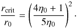 (24)For η0 = 1 we recover rcrit = r0, as expected. From the limiting case η0 ≫ 1 (i.e., a very dense parent belt), we find
 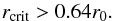 (25)This shows that far enough inward from the parent belt, P–R drag always dominates collisions. Furthermore, if Eq. (22) holds we find rcrit ≳ 12.8rpile, which means that in systems where the parent belt is distant enough for significant dust pile-up to occur, P–R drag dominates collisions in the sublimation zone, and collisions are so infrequent there that they do not interfere with the pile-up process.
The pile-up of dust means that τgeo increases around rpile, locally decreasing the collisional timescale. However, a significant pile-up requires Eq. (22) to hold, in which case the ratio between the minimum collisional timescale and the P–R drag timescale is found to satisfy ![Mathematical equation: \hbox{$ \min \left[ t\sub{coll}(r\sub{pile}) \right]/t\sub{PR}(r\sub{pile}) = 4 ( \sqrt{ r\sub{0}/r\sub{pile} } - 1 ) \gtrsim 13.9 $}](/articles/aa/full_html/2014/11/aa22090-13/aa22090-13-eq136.png) . To overcome this difference, the pile-up would have to raise τgeo by the same factor. Since the τgeo enhancement factor is never found to be greater than about 10 (Kobayashi et al. 2009), we expect the disk to remain drag (or sublimation) dominated inside rcrit.
. To overcome this difference, the pile-up would have to raise τgeo by the same factor. Since the τgeo enhancement factor is never found to be greater than about 10 (Kobayashi et al. 2009), we expect the disk to remain drag (or sublimation) dominated inside rcrit.
2.3.2. Estimating the pile-up magnitude
The efficiency of dust pile-up was studied in detail by Kobayashi et al. (2009, 2011), who give formulae for the resulting enhancement in particle number density and geometrical optical depth. Here, we present a simple order-of-magnitude estimate of the maximum amount of material in the pile-up, which can be used to assess whether pile-ups can explain the observed NIR excess emission.
Dust grains reside in the pile-up for roughly one sublimation timescale, after which they are either completely sublimated or their size is reduced so much that they are blown out of the system. Since the pile-up occurs roughly at rpile, defined such that tsubl(rpile) = tPR(rpile), the dust stays in the pile-up for about one P–R drag timescale. Given this, the total number of particles in the pile-up is 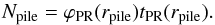 (26)To describe the radial profile in terms of geometrical optical depth, it is necessary to specify the radial width of the pile-up Δrpile. In reality, Δrpile depends on the orbital eccentricities of the particles in the pile-up and on differences in pile-up distance for particles of different sizes that contribute. Since this is beyond the scope of this work, we keep the relative pile-up width Δrpile/rpile as a free parameter.
Combining Eqs. (1), (6), and (26), we find that the geometrical optical depth due to the material in the pile-up is given by 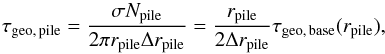 (27)where τgeo, base(r) denotes the base level of dust due to P–R drag and collisions given by Eq. (4). Kobayashi et al. (2009) find that sublimating dust particles slowly move outward. Therefore, we assume that the pile-up extends from rpile outward, overlapping with the inward migrating material. The complete geometrical optical depth profile, which includes the effects of collisions, P–R drag, and sublimation, can then be formally described by (cf. Kobayashi et al. 2011)
  (28)Using Eq. (5) for τgeo, base(r) gives the maximum profile. Figure 3 shows this maximum profile for different values of Δrpile/rpile.
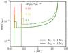 |
Fig. 3 Maximum geometrical optical depth profiles of debris disks with collisions, P–R drag, and sublimation (Eq. (28) with τgeo, base(r) given by Eq. (5)), for different values of relative pile-up width Δrpile/rpile shown in different colors. The solid lines correspond to disks around solar-mass stars, the dashed lines to disks around 2 M⊙ stars. All profiles assume a parent belt at r0 = 30 AU, dust grains with β = 0.5, and rpile ≈ 0.019 AU, and rpile ≈ 0.064 AU, for the M⋆ = 1 M⊙, and M⋆ = 2 M⊙ cases, respectively, corresponding to spherical graphite grains with β = 0.5. |
We can make a rough estimate of the geometrical optical depth enhancement factor fτgeo of the pile-up (i.e., how much higher τgeo in the pile-up is compared to the base level of the inner disk), as a function of the radial width of the pile-up Δrpile: 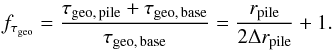 (29)For a pile-up width of Δrpile ≈ 0.05rpile (Kobayashi et al. 2011), this gives fτgeo ≈ 11, which is comparable to the highest values found by Kobayashi et al. (2009, see their Fig. 6) for carbonaceous dust grains around early F-type stars.
For comparison with observations, it suffices to assume that all the pile-up material is located at rpile (i.e., Δrpile/rpile ≪ 1). This gives the highest possible temperature to all pile-up particles, and therefore results in the maximum NIR flux. In the τgeo profile, however, it would give a singularity at r = rpile. To avoid this, we instead compute the fractional luminosity of the pile-up. Fractional luminosity is defined as the ratio of the infrared luminosity of the dust LD to the stellar luminosity. Assuming the disk is radially optically thin and the dust grains have unity absorption and emission efficiencies at all wavelengths (i.e., assuming black-body grains), it can be approximated by the fraction of the star that is covered by dust  (30)Evaluating this with n(r)dr = Npile, and using the maximum geometrical optical depth (Eq. (5)), we find that the maximum fractional luminosity due to material in the pile-up is
 ![Mathematical equation: \begin{equation} \label{eq:max_fraclum_pr} \max \left[ \left( \frac{ L\sub{D} }{ L\sub{\star} } \right)\sub{pile} \right] = \frac{ \sqrt{ G M\sub{\star} } \, \beta }{ 8 c \left( \sqrt{ r\sub{0} } - \sqrt{ r\sub{pile} } \right) }\cdot \end{equation}](/articles/aa/full_html/2014/11/aa22090-13/aa22090-13-eq160.png) (31)In the limit of r0 ≫ rpile, this becomes
(31)In the limit of r0 ≫ rpile, this becomes ![Mathematical equation: \begin{equation} \label{eq:max_fraclum_pr_r0} \max \left[ \left( \frac{ L\sub{D} }{ L\sub{\star} } \right)\sub{pile} \right] \approx 6.2 \times 10^{-6} \, \left( \frac{ M\sub{\star} }{ {1~M}\sub{\odot} } \right)^{1/2} \, \left( \frac{ r\sub{0} }{ \mathrm{1~AU} } \right)^{-1/2} \, \left( \frac{ \beta }{ 0.5 } \right)\cdot \end{equation}](/articles/aa/full_html/2014/11/aa22090-13/aa22090-13-eq162.png) (32)This is only the fractional luminosity due to the dust in the pile-up. Material just beyond rpile is not accounted for, and will increase the total fractional luminosity.
(32)This is only the fractional luminosity due to the dust in the pile-up. Material just beyond rpile is not accounted for, and will increase the total fractional luminosity.
2.4. Summary of analytical findings
The analytical model presented above yields several tentative conclusions about dust in the inner parts of debris disks:
-
1.
P–R drag gives rise to a small but non-zero inward mass flux ofdust in the inner disk, which is self-limited by collisions(Eq. (11)).
-
2.
A pile-up of sublimating dust occurs, as long as the star is luminous enough (Eq. (18)), and the parent belt is distant enough (Eq. (22)).
-
3.
P–R drag dominates collisions in the inner parts of the disk (Eq. (25)), so collisions do not interfere with dust pile-up.
-
4.
Given that the pile-up of dust occurs around the radial distance where the sublimation timescale equals the P–R drag timescale and that sublimating dust resides in the pile-up for about one sublimation timescale, there is a maximum fractional luminosity that this dust can provide (Eq. (32)).
3. Numerical modeling
The analytical approach used in Sect. 2 contains several simplifying assumptions. Most importantly, we only self-consistently solve the continuity equation for P–R drag and collisions (under the assumptions listed in Sect. 2.1), and afterwards estimate the effect of dust pile-up due to sublimation, assuming the grains reside in the sublimation zone for one P–R drag timescale (see Sect. 2.3.2). To test the impact of these assumptions, we now proceed to solve the continuity equation numerically using a debris disk model that self-consistently handles the effects of stellar gravity, direct radiation pressure, P–R drag, sublimation, and destructive collisions. Our strategy here is to simulate a few specific cases and compare the results to the analytical maximum distributions found in Sect. 2, to assess the validity and generality of these simple expressions. A description of our numerical debris disk model is given in Sect. 3.1, the runs we performed are detailed in Sect. 3.2, and the resulting dust distributions are presented in Sect. 3.3.
3.1. Model description
Our debris disk model closely follows the method developed by Krivov et al. (2005, 2006) and Löhne (2008). We refer the reader to these publications for a detailed description of the method and only provide a brief outline of its principles here. We focus on the changes we made, which are including a time-dependent treatment of dust sublimation (see Sect. 3.1.3) and implementing additional numerical acceleration techniques (see Appendix A). Our code was tested by comparing its predictions to solutions of the equations of motion and sublimation for individual particles and by benchmarking it against the results of Krivov et al. (2006). This verification is described in Appendix B. Two physical processes that are included by Löhne (2008), but not considered by our present code, are stellar wind drag and erosive (cratering) collisions. We discuss the impact they may have on our results in Sect. 5.
3.1.1. Method basics
The method of Krivov et al. (2005) applies the kinetic method of statistical physics to debris disks, simultaneously following the spatial and size distributions of dust and planetesimals in a phase space of orbital elements and particle masses. Using orbital element instead of radial distance to follow the spatial distribution makes it possible to account for particles on eccentric orbits, whose orbits can span a wide range of radial distances. The continuity equation is solved in this phase space, with processes that affect the evolution of a particle’s phase-space coordinates in a continuous fashion (P–R drag and sublimation) as diffusion terms, and processes that abruptly change phase-space coordinates (collisions) as source and sink terms. Formally, this is decribed by (cf. Krivov et al. 2005; Löhne 2008)  (33)where n(m,k,t) is the phase-space number density at time t (i.e., the distribution function that describes the state of the disk), k the vector of orbital elements, and { m,k } denotes the vector consisting of m and k. The divergence term represents the diffusion of material in phase space (i.e., transport due to P–R drag and sublimation). For brevity, we omit the arguments (m,k,t) for all terms on the righthand side of the equation.
To make the numerical evaluation of the continuity equation manageable with limited computational capacity, the number of phase-space variables needs to be reduced. By assuming the disk is axisymmetric, the distribution function can be averaged over three of the orbital elements: longitude of the ascending node, argument of the periastron, and true anomaly. This implicitly assumes that collisional timescales are much longer than orbital timescales, which generally holds for debris disks (for a more detailed discussion, see Sect. 3.1.3 of Löhne 2008). A further assumption is that the distribution of particles over inclinations is constant, which allows the averaging of the distribution function over inclination. The three remaining phase-space variables are (1) particle mass m; (2) orbital eccentricity e; and (3) an orbital element characterizing the size of the orbit, such as semi-major axis a or periastron distance q = a(1 − e).
The final phase-space variable can be chosen to fit the numerical needs of the problem under investigation. For our study of the pile-up of dust due to sublimation, we chose periastron distance. A particle on an eccentric orbit experiences most sublimation around the periastron, owing to the strong temperature dependence of sublimation. Since the periastron distance does not evolve for β changes that happen at the periastron, the orbit’s periastron distance changes much more slowly than its semi-major axis. Using q instead of a as phase-space variable therefore has numerical advantages.
In practice, the phase space is divided into a grid of bins, and the distribution function is replaced by a vector listing the number of particles in each bin. Equation (33) then becomes a system of ordinary differential equations. The source, sink, and diffusion terms are discretized, and they determine the rates at which the particle numbers evolve, dependent on the population levels of other bins. We now proceed to describe these terms for each of the physical processes considered by our model.
3.1.2. Poynting–Robertson drag
P–R drag affects the orbits of particles, circularizing them, and making them smaller. These effects are accounted for in the model by diffusion terms in the continuity equation that move particles to adjacent bins in the phase-space grid. Since the P–R drag timescale is usually longer than the orbital period, we use the orbit-averaged change rates of the orbital elements, given by (e.g., Burns et al. 1979)  For the rate of change in periastron distance, we find
3.1.3. Sublimation
The formalism that we use for dust sublimation is described in Sect. 2.2.1. For a spherical dust particle, it gives a mass loss rate of  (38)In our numerical model, we use realistic dust grain temperatures (as opposed to the black-body temperatures used in Sect. 2). The method for computing these temperatures is explained in Sect. 3.2.2.
Since the sublimation rate strongly depends on grain temperature, which varies along the path of an eccentric orbit, the mass loss rate needs to be averaged over the orbit. As described qualitatively in Sect. 2.2.2, the change in β ratio associated with mass loss induces changes in orbital elements. Kobayashi et al. (2009) derive the orbit-averaged change rate in orbital elements and mass to be 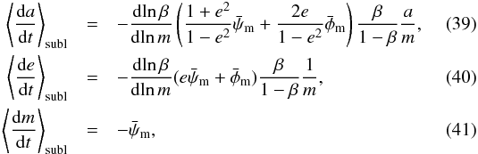 with
with 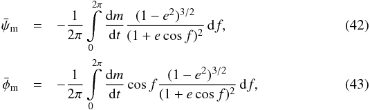 where f denotes the true anomaly. For the periastron distance, we find
 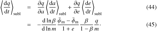 For each phase-space bin, quantities
  and
and  are numerically evaluated using the standard Euler method9. The change rates of the phase-space variables (Eqs. (40), (41), and (45)) are then used in diffusion terms in the continuity equation.
Using orbit-averaged mass loss rates is only correct if the sublimation timescale is longer than the orbital period. For phase-space bins for which this does not hold (small particles close to the star), we compute an equilibrium population of particles from the product of their sublimation timescale and the sum of their gain terms. This implicitly assumes that particles are created on their orbits with a uniform distribution over true anomaly.
3.1.4. Collisions
Collisions are different from P–R drag and sublimation in that they cause abrupt rather than smooth changes in phase-space coordinates. In the continuity equation, they are described by sink terms at the phase-space coordinates of targets and projectiles and by source terms at the coordinates of the resulting fragments. Here, we give a summary of the way our model handles collisions. More thorough descriptions of the treatment of collisions, including all relevant equations, are given by Krivov et al. (2006) and Löhne (2008).
For each pair of phase-space bins, we determine collision rates for a range of relative orbit orientations (differences in the longitudes of the periastra of the two orbits). The collision rate is the product of the target and projectile number densities, their relative velocity, the collisional cross-section, and the effective volume of interaction. Krivov et al. (2006) found analytical expressions for these factors in two dimensions as a function of the orbital elements and masses corresponding to both bins and the relative orientation of the orbits. To account for the third dimension, a correction is applied based on the semi-opening angle of the disk, equivalent to the maximum inclinations of the particles. This correction assumes that the disk is relatively flat, consistent with observations of resolved edge-on systems.
To save computational power, we ignore collisions involving unbound particles. This is a valid approximation if the radial geometrical optical depth of the system is much smaller than unity (true for most debris disks), because then the blowout timescale of such particles is much shorter than their collisional timescale10.
The nature of a collision is determined by the impact energy available per unit of mass. We only consider catastrophic collisions, defined as destructive events in which the largest fragment contains at most half of the mass of the more massive of the two impactors. The threshold for these catastrophic collisions is the critical specific energy for dispersal  , which incorporates the fact that fragments may reassemble after destruction, and generally depends on particle size. If the specific energy of a collision is higher than this threshold, the impact destroys both bodies, and their mass is distributed over a swarm of fragments. At specific energies just below , collisions are erosive. Such cratering collisions, however, are not considered in our present model, so if the specific energy of an impact is lower than , no collision is considered to occur.
A catastrophic collision results in a range of fragments with different masses and orbits. The fragments are distributed over particle masses according to a single power law, up to a maximum fragment mass, which is determined by the kinetic energy of the impact and the material strength of the target. The maximum fragment mass is at most half of the mass of the target and projectile combined, but it can also be less, if the specific energy involved in the collision is more than . The amount of particles that end up in each mass bin (up to the maximum fragment mass) is computed by integrating the fragment mass distribution. Particles with masses below the lowest mass bin (i.e., that fall off the grid) are considered lost due to immediate blowout or vaporization. For each fragment mass bin, new orbital elements are calculated using the conservation of momentum, and taking into account direct radiation pressure (i.e., the values of β of the fragments), using Eqs. (19) and (20) of Krivov et al. (2006). This assumes that the fragments are not launched away from the collision with any velocity. These orbital elements are rounded to the nearest periastron distance and eccentricity bins for each fragment mass bin.
3.2. Setup of the model runs
3.2.1. Stellar and disk parameters
Hot exozodiacal dust has been detected around stars with spectral types ranging from A to K (see Table 1). To focus on this range of stellar types, we did one model run with a solar-mass star and one using a 2 M⊙ star. Following the mass–luminosity relation for main-sequence stars (L⋆ ∝ M⋆3.5; Allen 1976), we set the stellar luminosities corresponding to these stellar masses to L⋆ = 1 L⊙ and L⋆ = 11.31 L⊙, respectively.
Both runs use a parent belt radius of r0 = 30 AU. Lower values of r0 can in principle yield higher dust levels in the innermost regions (see Eq. (5)), but parent belts closer to the star are generally not dense enough to provide these large amounts of dust, because they do not survive the intense collisional grinding (Dominik & Decin 2003; Wyatt et al. 2007). In addition, many of the observed outer belts are located at tens of AUs (see Table 1). The level of dust in the source region is set to τgeo(r0) ≈ 5 × 10⁻⁵, chosen such that (i.e., iterated until) the geometrical optical depth in the inner regions does not become any higher by increasing the level of dust at the source11. This roughly corresponds to η0 ~ 10 for both stellar mass cases, which is apparently enough to approximate an inner disk τgeo profile corresponding to η0 ≫ 1. For the semi-opening angle of the disk we use ε = 8.5°.
3.2.2. Material properties
We consider carbonaceous dust particles with a density of ρd = 1.8 g cm-3. To compute the optical properties of these grains with different radii, we use the DHS method of Min et al. (2005) with an irregularity parameter of fmax = 0.8. This method simulates the properties of irregularly shaped particles. For the material we use amorphous carbon with the refractive index data taken from Preibisch et al. (1993). These optical properties are used to compute β(s) and dust temperatures. The dust temperatures are computed by solving the balance between absorption and thermal emission as a function of grain size and distance to the central star. For the sublimation properties, we use those of graphite, given in Sect. 2.2.1.
Modeling collisions requires a prescription for the specific energy threshold for dispersal  , which is generally found to depend on size. In our numerical simulation, we consider particles with radii up to 1 cm. (see Sect. 3.2.4). For bodies smaller than s ~ 100 m, is often described by a power law with a negative exponent (e.g., Benz & Asphaug 1999). However, such a prescription predicts unrealistically high values for the small particles that we consider. Therefore, following Heng & Tremaine (2010), we use the constant value of
  erg g-1 found in laboratory experiments with high-velocity collisions of small particles (Flynn & Durda 2004). We follow Krivov et al. (2006) in setting the collisional fragment mass distribution to n(m) ∝ m−11 /6, and in assuming the maximum fragment mass scales with specific impact energy to the power −1.24 (Fujiwara et al. 1977).
3.2.3. The phase-space grid
Because this problem is computationally very demanding, great care has to be taken in setting up the phase-space grid. Specifically, resolving the pile-up requires high resolution in the sublimation zone and at small particles sizes, where radiation pressure becomes important. To achieve this with limited computational resources, we designed a non-uniform grid that has a higher resolution where it is required.
The eccentricity grid contains ten logarithmic bins between e = 0 and e = 1, with the lowest bin at e = 10-4. In addition, there are two linearly spaced eccentricity bins between e = 1 and e = 2 for hyperbolic orbits, as well as two bins between e = −2 and e = −1 to account for “anomalous” hyperbolic orbits followed by β> 1 particles (see Krivov et al. 2006).
The periastron distance grid consists of two parts: (1) a high-resolution, linear grid of 21 bins is used to cover the sublimation zone (0.01 AU <q< 0.03 AU for the M⋆ = 1 M⊙ run, and 0.05 AU <q< 0.1 AU for the M⋆ = 2 M⊙ run). (2) A low-resolution, logarithmic grid covers the rest of the disk out to about q = 100 AU, with 60 bins in the M⋆ = 1 M⊙ run and 50 bins in the M⋆ = 2 M⊙ run. Care was taken to place one bin exactly at q = 30 AU, which was used as the source region.
The mass grid has 48 logarithmically spaced bins in both runs with higher resolution at the smaller sizes (β ≳ 0.05) and a maximum mass corresponding to s = 1 cm. For the M⋆ = 1 M⊙ run, the high-resolution part consists of 30 bins between s = 0.5 μm and s = 10 μm. The high-resolution part of the M⋆ = 2 M⊙ run has 36 bins between s = 2 μm and s = 100 μm.
3.2.4. Simulation strategy
Owing to computational limitations, the largest particles we consider have a radius of 1 cm. In reality, the size distribution in the parent belt extends up to planetesimals of tens to hundreds of kilometers. To account for the fragmentation of these larger bodies, we include a source of dust at r0. This artificial source term adds particles with sizes between s = 1 mm and s = 1 cm, following the power-law size distribution n(s) ∝ s-3.5. The size of these grains is chosen such that the effect of radiation pressure on them is very small (β< 10-4). Therefore, their eccentricity distribution follows that of the parent bodies. We add the source particles at eccentricities ranging from e = 0 to e = 0.1.
The artificial supply of large dust particles is balanced by the loss of material due to blowout and sublimation. Therefore, solving the continuity equation results in a steady-state distribution function. We start the integration without any material in the disk (only the artificial supply is acting) and let the model run until steady state is reached. This is considered to be the case when relative changes in the radial and size distributions between logarithmic (base-10) time steps become less than 1%12. Initially, we only consider collisions and P–R drag, and the sublimation module of the code is switched off. At this stage, particles migrate inward due to P–R drag until they reach the inner edge of the grid. Once steady state is reached, sublimation is switched on, and we let the distribution function settle into a new steady state. This procedure is necessary because sublimation forces the time step to become very short. With sublimation switched on from the start, the computation would take unnecessarily long. Additionally, it allows us to isolate the effect of dust pile-up (i.e., the dust in the pile-up can be isolated by subtracting the pre-sublimation state from the final one).
3.3. Results
The output of each model run is a steady-state distribution of particles in the phase space of orbital elements and masses. To analyze this output, we convert it into a radial geometrical optical depth profile (Sect. 3.3.1) and size distributions (in terms of cross-section density per unit size decade A) at different radial locations (Sect. 3.3.2). The conversion from raw model output to these quantities is detailed in Appendix C.
3.3.1. Radial distribution
Figure 4 shows the geometrical optical depth profiles derived from the numerical model runs, together with the analytical maxima given by Eq. (28), using a pile-up width of Δrpile/rpile = 0.15, chosen to match the numerical profile. Generally, there is good correspondence between the numerical results and the analytical maxima, but there are some important differences. The profiles have roughly the same shape, with a slightly steeper slope close to the source region in the numerical results. For both cases of stellar mass, the base level of τgeo in the inner disk (i.e., away from the pile-up) is a factor of about 7 lower in the numerical profiles. This discrepancy is a result of the the assumption in the analytical model that all orbits are circular. In the numerical model, the small particles that contribute most to the cross-section are released in the parent belt on eccentric orbits. They therefore suffer a higher rate of destruction by collisions.
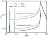 |
Fig. 4 Geometrical optical depth profiles of debris disks with a dense parent belt at 30 AU around stars of M⋆ = 1 M⊙ (solid lines) and M⋆ = 2 M⊙ (dashed lines). The black lines show the end results of the numerical simulations. In green are the maximum τgeo profiles as given by the analytical model (Eq. (28), with τgeo, base(r) given by Eq. (5), Δrpile/rpile = 0.15, r0 = 30 AU, and β = 0.5). |
As predicted, switching on sublimation leads to an accumulation of dust. The pile-ups are located very close to rpile, as determined for graphite grains, using black-body temperatures and Qpr = 1 (Eq. (17), which gives rpile ≈ 0.019 AU for the M⋆ = 1 M⊙ case, and rpile ≈ 0.064 AU for the M⋆ = 2 M⊙ case). The temperature of the dust (as computed using the full optical properties) at the inner edge of the disk and in the pile-up is between 2000 and 2100 K. In both runs, the pile-up has a geometrical optical depth enhancement factor of about fτgeo ≈ 3. The fractional luminosities due to the pile-ups are (LD/L⋆)pile ≈ 7.5 × 10⁻⁸ for the M⋆ = 1 M⊙ case and (LD/L⋆)pile ≈ 1.1 × 10⁻⁷ for the M⋆ = 2 M⊙ case. Both are about a factor 15 lower than the maxima given by Eq. (32). Given that the base levels of τgeo in the numerical profiles are a factor of about 7 lower than the analytical maxima, however, the discrepancy is only about a factor of 2. In short, the pile-up mechanism is found to be somewhat less efficient than predicted by the analytical estimates.
The outer disk (r> 30 AU) is not the focus of this work. Nevertheless, its radial profile is relevant, since it reflects the status of the balance between collisions and P–R drag. To first order, the geometrical optical depth profile of the outer disk can be characterized by a power law τgeo ∝ r−α. Strubbe & Chiang (2006) derive the theoretical values of α = 1.5 and α = 2.5 for collision and P–R drag-dominated disks, respectively. We find slopes of α ≈ 2.0 for both runs, consistent with the outer slope found by Vitense et al. (2010) for the Edgeworth–Kuiper Belt, and interpreted as the sign of a disk that is in between drag and collision-dominated. This indicates that the density of the parent belt (characterized by η0 ~ 10) is insufficient to make the outer disk completely collision-dominated.
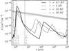 |
Fig. 5 Size distributions at different radial distances for the M⋆ = 1 M⊙ run before switching on sublimation. The quantity on the vertical axis, A, is the cross-section density per unit size decade (see Appendix C.2), which is horizontal if all sizes contribute equally to the cross-section. The gray band indicates the slope of a size distribution that follows the classical Dohnanyi (1969) power law (n(s) ∝ s-3.5, hence A ∝ s-0.5). The vertical lines mark the particle sizes corresponding to relevant values of β. |
3.3.2. Size distribution
The size distribution results of the two runs are similar in many ways, so we only discuss the M⋆ = 1 M⊙ run here. Figure 5 shows how the size distribution changes with radial distance when only considering P–R drag and collisions (i.e., before sublimation is switched on in the model). In the parent belt (r = 30 AU), it follows the classical Dohnanyi (1969) power law (n(s) ∝ s-3.5, which is valid for an infinite collisional cascade with self-similar collisions), from the blowout radius upwards. Particles with β> 0.5 are depleted by about three orders of magnitude in terms of collective cross-section. Superimposed on the power law is a well-known wave pattern related to the discontinuity in the size distribution at the blowout size (see, e.g., Campo Bagatin et al. 1994; Durda & Dermott 1997; Gáspár et al. 2012). The first bump (i.e., the one at β ≈ 0.5) in the size distribution at r = 30 AU does not extend far above the power-law prediction. The reason for this may be that particles with β ≳ 0.1 experience more destructive collisions, because their eccentricities are significantly higher than those of the parent bodies, which are distributed over the range 0 <e< 0.1 (Sect. 3.2.4, see also Eq. (19), and cf. Fig. 5 of Krivov et al. 2006).
Inward from the parent belt, the size distribution seems to become steeper, which is expected from the dependence of the radial profile on β (Eq. (5)). However, this effect is difficult to isolate, because the profile is distorted by the wave pattern, which increases in amplitude and “wavelength” with decreasing radial distance (cf. Fig. 7 of Krivov et al. 2006). The prominent wave pattern indicates that collisions are still important for larger particles in the inner disk (while P–R drag dominates for β ≈ 0.5 particles there, see Fig. 2). In the innermost parts of the disk (r ≲ 1 AU), particles with β ≈ 0.5 clearly dominate the cross-section, contributing at least three orders of magnitude more than any other size. At r = 0.1 AU, the local slope of the size distribution between the blowout size and s ≈ 10 μm is approximately A ∝ s-7.5, equivalent to n(s) ∝ s-10.5. This means that not only the cross-section, but also the mass is dominated by barely bound grains in the innermost parts of the disk. Interestingly, such steep size distributions are also invoked to explain NIR interferometric observations of hot exozodiacal dust (Defrère et al. 2011; Mennesson et al. 2013; Lebreton et al. 2013). The drop in the size distribution from β ≈ 0.5 to β ≈ 1 is also much more pronounced in the inner disk than in the parent belt.
Sublimation only has a significant effect on the size distribution around r ≈ rpile (i.e., in the pile-up). Figure 6 shows the size distribution in the pile-up, before and after sublimation is switched on. It clearly demonstrates that sublimation enhances the density of particles with 0.5 ≲ β< 1 around r = rpile. This indicates that the pile-up consists mostly of particles that started with β ≈ 0.5 before active sublimation and lost mass due to sublimation, increasing their β. The rest of the size distribution does not change significantly. Size distributions at larger radial distances are largely unaffected by sublimation.
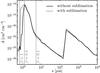 |
Fig. 6 Size distribution at r = 0.02 AU (the location of pile-up) for the M⋆ = 1 M⊙ run, before and after sublimation is switched on. |
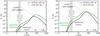 |
Fig. 7 SEDs of stars and their debris disks at a distance of 10 pc. The disk SED is shown for different dust distributions with the numerical results in black and the analytical distributions in green. Dust distributions including the pile-up of dust in the sublimation zone are shown with dashed lines, and distributions in which the pile-up is excluded are shown with solid lines, but the spectra largely overlap. Disk SEDs are calculated according to Eqs. (46) and (47). The stellar photosphere is indicated by a dotted Planck curve. The vertical gray areas mark the NIR H and K bands in which hot exozodiacal dust is observed. |
4. Comparison with observations
To assess whether the pile-up effect can explain the observed NIR excess, we computed the spectral energy distributions (SEDs) of the dust distributions found in the previous sections. We only calculated the emission spectrum of the dust and ignored the (viewing-angle-dependent) contribution of scattered light, since thermal emission was found to dominate scattered light at the wavelengths in which hot exozodiacal dust is detected (Absil et al. 2006). For the analytical dust distributions, we assumed the dust has a black-body temperature (Eq. (14)). The flux density of the dust, expressed as a function of wavelength λ, can then be computed as 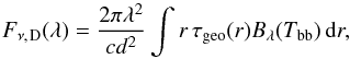 (46)where d is the distance to the source, and Bλ(T) the Planck function. For the numerically determined dust distributions, we use realistic dust temperatures and optical properties (see Sect. 3.2.2), which leads to
 ![Mathematical equation: \begin{equation} \label{eq:sed_dust_num} F_{\nu,\;\!\mathrm{D}}(\lambda) = \frac{ 2 \pi \lambda^2 }{ c d^2 } \int\limits_{s} \! \! \! \int\limits_{r} r Q\sub{abs}(s) \, \tau\sub{geo}(s,r) B_\lambda[T(s,r)] \, \dif s \, \dif r. \end{equation}](/articles/aa/full_html/2014/11/aa22090-13/aa22090-13-eq256.png) (47)Here, Qabs is the absorption efficiency of the grains (equal to their emission efficiency) and τgeo(s,r) is the geometrical optical depth profile of dust with grain radius s.
(47)Here, Qabs is the absorption efficiency of the grains (equal to their emission efficiency) and τgeo(s,r) is the geometrical optical depth profile of dust with grain radius s.
Figure 7 shows the debris disk spectra corresponding to dust distributions found from the numerical modeling, as well as the analytical maximal dust profiles and the stellar spectra. The analytical maxima are computed from Eq. (28), with τgeo, base(r) given by Eq. (5), r0 = 30 AU, β = 0.5, and all the pile-up material at rpile (i.e., Δrpile/rpile ≪ 1)13. Singularities at r = r0 are removed by imposing the condition τgeo ≤ 0.01, which corresponds to η0 ≈ 2200. The numerical dust distributions without pile-up were created by subtracting the isolated pile-up dust from the final profile (see Sect. 3.2.4). The stellar spectra are given by black-body curves, with L⋆ = 1 L⊙, T⋆ = 5780 K for the M⋆ = 1 M⊙ star, and L⋆ = 11.31 L⊙, T⋆ = 7730 K for the M⋆ = 2 M⊙ star, following the main-sequence relations L⋆ ∝ M⋆3.5 and T⋆ ∝ L⋆0.12 (Allen 1976). The distance is arbitrarily set to 10 pc.
The synthetic spectra are similar to those described by Wyatt (2005), but are truncated at short wavelengths because there is no material with a higher temperature than the sublimation temperature. Apart from an overall shift in flux, the differences between the analytical and numerical SEDs are minor. In the solar-mass star run, the peak of emission of the numerical result is shifted toward shorter wavelengths with respect to the analytical SED. This is because the grains that dominate the emission in the parent belt are significantly hotter than the black-body temperature.
Only considering thermal emission, the NIR flux originates almost exclusively in the inner 1 AU of the debris disk. The pile-up does not add a significant amount of flux. The theoretical SEDs display NIR flux ratios between the disk and star of about Fν,D/Fν,⋆ ~ 10-4. This is much less than the observed flux ratios that indicate hot exozodiacal dust, which are typically on the order of 1% (see Table 1). Furthermore, the NIR radiation is accompanied by mid-IR flux at a comparable level, which is incompatible with observed excess spectra (e.g., Akeson et al. 2009). The pile-up does not contain enough material to create a bump in thermal flux in the NIR.
To generalize the above results, we investigate how the NIR flux ratio depends on parent belt distance and stellar type using the analytical model. In Fig. 8, we show the analytical maximum NIR flux ratios for four different stellar types. As in the above analysis, the disk flux is calculated from Eq. (46), using the analytical maximum dust distribution, and the stars are approximated by black bodies. The M0V, G2V, A5V, and B5V stars correspond to M⋆ = 0.5, 1, 2, and 4 M⊙, respectively, with L⋆ ∝ M⋆3.5 and T⋆ ∝ L⋆0.12 (Allen 1976). Comparing the analytical maximum NIR flux ratios to the observed ones demonstrates that P–R drag does not provide enough material to the inner disk to explain the observations.
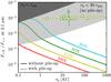 |
Fig. 8 Flux ratio between the disk and the star at 2.1 μm (K band), as function of parent belt radius r0. Solid lines indicate the flux ratio due to the maximum amount of material moved in by P–R drag, truncated at r = rpile. Ratios including the small effect due to pile-up are shown with dashed lines. Different colors are used for different stellar types. The light shaded area marks the region in parameter space where no significant pile-up is expected to occur because the orbits of small dust grains cannot circularize sufficiently (see Eq. (22)). The dark shaded area marks where the parent belt r0 is closer than the pile-up radius rpile. The observed K-band excess fluxes of main-sequence stars from Table 1 are shown at their respective estimated parent belt distances with a different symbol for each star and coloring according to the star’s spectral type: Vega (the CHARA/FLUOR measurement): circles; β Leo: hexagon; Fomalhaut: squares; β Pic: diamond; η Lep: upward pointing triangles; 110 Her: left-pointing triangle; 10 Tau: right-pointing triangle; τ Cet: pentagon. |
5. Discussion
5.1. The size distribution in the inner disk
The size distribution in the inner parts of dense debris disks (i.e., inward from the parent belt) has not been studied many times before. Acke et al. (2012) analytically derive a power-law distribution of n(s) ∝ s-3, but ignore collisions in the inner disk. In a detailed modeling study of the debris disk around ε Eri, Reidemeister et al. (2011) find a flat profile (n(s) ∝ s-3, flat in terms of A) for small sizes, and a steeper one (n(s) ∝ s-3.7) for larger sizes. However, this system is a special case, because ε Eri is not luminous enough to blow small dust grains out of the system.
With our numerical model, we find a size distribution that deviates significantly from a power law. Specifically, in the innermost regions of the disk (r ≲ 1 AU), the cross-section is completely dominated by barely bound (β ≈ 0.5) particles. This is the result of two effects: (1) Since the efficiency of P–R drag depends on β, larger particles tend to stay closer to the parent belt (apparent from Eq. (5)). (2) Owing to the high relative velocities in the inner disk14, the wave in the size distribution is extremely strong. As a consequence, the single size assumption used in our analytical model is a good approximation.
Erosive (cratering) collisions affect the size distribution (Thébault & Augereau 2007). We expect that including this type of collisions in our model would result in a less wavy size distribution, possibly eliminating the second bump in the size distribution (see Sect. 4.3.4 of Löhne 2008). This would mean that β ≈ 0.5 particles dominate the cross-section even more than suggested by Fig. 5. Since erosive collisions present an additional mechanism for destroying dust, we expect that including them in our model would only lower the level of dust in the inner disk, so it does not change the conclusions of this work. Erosive collisions do affect the timescale on which debris disks evolve, but since we compute steady-state dust distributions, this does not have any impact on our results.
It may be surprising that a large number of particles are present in the pile-up with 0.5 ≲ β< 1. Usually (as in Sect. 2), particles with β> 0.5 are assumed to be absent, because they are blown out of the system as soon as they are released from parent bodies on circular orbits. Parent bodies on eccentric orbits can give rise to a population of bound grains with β> 0.5, but the parent body orbits in our model runs are not eccentric enough to produce bound dust grains with β values close to unity. The origin of this high β population is the sublimation of barely bound β ≈ 0.5 grains. As these particles migrate inward from the parent belt, their orbits are circularized by P–R drag. When they arrive in the sublimation zone, their orbital eccentricities are as low as e ≈ 10-4. Kobayashi et al. (2009) find that the subsequent evolution of the eccentricities during the active sublimation phase can be described by  (48)where subscript 1 denotes quantities at the start of substantial sublimation, and the exponent κ can be treated as a constant, which mostly depends on the optical and sublimation properties of the material under consideration. For spherical, black-body graphite particles, we find κ ≈ 10. This shows that particles starting with β1 ≈ 0.5, and e1 ≈ 10-4 will only become unbound (e ≥ 1) when they reach β ≳ 0.8 (corresponding to s ≈ 0.8 μm).
5.2. Stellar wind drag
Neither our analytical nor our numerical model includes the effects of stellar wind. For stars with a strong stellar wind and/or low luminosity, the stellar wind equivalent of P–R drag shortens the inward migration timescale and thus increases the maximum geometrical optical depth profile. Since stellar wind drag works in the same way as P–R drag, its effect can be accounted for by replacing β with (Burns et al. 1979; Minato et al. 2004, 2006)  where Ṁ⋆ is the stellar mass loss rate by stellar wind, and Qsw is the stellar wind momentum transfer efficiency. For carbonaceous particles orbiting the Sun, Minato et al. (2004, 2006) find γ ~ 1.
Kobayashi et al. (2011) argue that the pile-up scenario could work for Vega if the disk is drag-dominated, which requires γ ≈ 300. While this value is consistent with the upper limit on the mass-loss rate of Vega from radio-continuum observations (Ṁ⋆ ≲ 10-10 M⊙ yr-1; Hollis et al. 1985), stellar wind models predict much lower mass-loss rates for main-sequence A-type stars (Ṁ⋆ ≲ 10-16 M⊙ yr-1; Babel 1995). This theoretical mass-loss rate, together with L⋆ ≈ 10 L⊙ and Qsw ≈ Qpr, gives a ratio between stellar wind drag and P–R drag of γ ≲ 10-4. We therefore conclude that it is unlikely that stellar wind drag has a significant effect on debris disks around main-sequence A-type stars.
5.3. Other explanations for hot exozodiacal dust
We find that P–R drag does not provide enough material to the innermost parts of the disk to explain the interferometric detections of NIR excess. There are two additional problems with this scenario, which also serve as clues for solving the hot exozodiacal dust mystery. (1) Hot exozodiacal dust is thought to consist mostly of blowout grains with sizes around 0.01–0.1 μm (Akeson et al. 2009; Defrère et al. 2011; Mennesson et al. 2013; Lebreton et al. 2013), while P–R drag only transports bound grains to the sublimation zone, the smallest of which have sizes of about 1 μm. (2) The dust distribution resulting from the balance between P–R drag and collisions yields an SED with a positive slope in the infrared domain, while observations find negative slopes (e.g., Akeson et al. 2009; Acke et al. 2012), and the pile-up of dust is too inefficient to have an effect on the slope of the SED15. For these reasons, the origin of hot exozodiacal dust must involve mechanisms that we did not consider in this work.
Our treatment of sublimation assumes spherical dust grains that sublimate uniformly (i.e., layers of material are removed one by one). In reality, dust grains may be aggregates that fall apart during sublimation, abruptly increasing the collective cross-section of the material. To investigate this scenario, the steady-state amount of material can be estimated by multiplying the maximum P–R drag inward mass flux (Eq. (11)) with an estimate of the lifetime of the fragments. We performed this analysis for Fomalhaut and find that P–R drag from a parent belt at 2 AU still does not supply enough material, unless the lifetime of the fragments is significantly longer than what can be expected from sublimation and blowout (Lebreton et al. 2013).
Two mechanisms have recently been proposed that can lead to an extended lifetime for small exozodiacal dust particles. Lebreton et al. (2013) investigate the impediment of blowout due to the presence of gas for the hot dust around Fomalhaut, but find that this requires unrealistically high gas densities. Su et al. (2013) propose that charged nanograins can remain trapped in the magnetic field of the star and qualitatively show that this may help explain the NIR excess of Vega.
Another mechanism for the inward transport of material from a cold outer belt is the inward scattering of material by planets. Bonsor et al. (2012) investigated this scenario and find that it is marginally capable of providing mass influxes compatible with observations. However, this requires relatively contrived planetary system architectures, consisting of closely packed chains of low-mass planets. Furthermore, the scenario was investigated for the inward scattering down to 1 AU, and reaching the sublimation zone is likely to be less efficient.
6. Conclusions
In this work, we investigated hot dust in the inner regions of debris disks, whose presence is suggested by interferometrically resolved excess NIR emission observed in some debris disk systems (Table 1). We tested whether the hot dust can be supplied by P–R drag from a distant parent belt and whether the pile-up of dust in the sublimation zone still occurs if collisions are considered. Our main conclusions follow.
-
1.
As predicted by Wyatt (2005), P–R drag al-ways brings a small amount of dust from an outer debris beltinto the sublimation zone. The maximum geometrical opticaldepth that can be reached in the innermost parts of the disk de-pends on the mass of the central star and distance to the parent belt(Fig. 1). When the production of dust is treatedself-consistently, this maximum is found to be a factor of about 7lower than the analytical estimate (Fig. 4). Thisis because small dust particles, which are efficiently draggedinward by radiation forces, are also put on highly eccentric orbitsby those radiation forces and therefore suffer more collisionaldestruction.
-
2.
Dust that reaches the sublimation zone produces some NIR emission, but this excess flux is insufficient to explain the interferometric observation. While the observed excess ratios are ~10-2, the maximum flux ratio due to material supplied by P–R drag is ≲10-3 for A-type stars with parent belts at ≳1 AU (Fig. 8).
-
3.
The pile-up of dust from the interplay of P–R drag and sublimation still occurs when collisions are considered (Fig. 4), as long as the parent belt in which the dust originates is distant enough to allow for sufficient circularization of the orbits, and the central star is luminous enough to blow small dust grains out of the system. Collisions do not interfere with the pile-up process, since in the inner disk, the collisional timescale is longer than the P–R drag timescale for the barely bound grains that are the most important for the pile-up. The fractional luminosity provided by dust in the pile-up is relatively low, so the pile-up does not influence the disk SED significantly (Fig. 7).
-
4.
In the inner parts of dense debris disks, the cross section is clearly dominated by barely bound (β ≈ 0.5) grains, and the size distribution features a prominent wave pattern, related to the discontinuity in the size distribution at the blowout size (Fig. 5). In the pile-up, there is an enhancement of particles with 0.5 ≲ β< 1 (Fig. 6). These particles are still bound, because of their almost circular orbits at the start of substantial sublimation.
Online material
Appendix A: Numerical techniques
Our model is computationally very demanding, primarily because of the large number of calculations needed for collisions, which scales with the number of phase-space bins cubed. To ensure that the model can produce results in a reasonable amount of time, an effort was made to reduce the amount of calculations needed per run. To achieve this, we used an integration technique that allows large time-step sizes, which reduces the number of steps needed per run (Appendix A.1). Furthermore, we calculated as many time-independent numerical factors as possible before the actual integration, so these factors do not have to be determined at every time step (Appendix A.2).
Appendix A.1: Integration method
After discretization, the distribution function n(m,k,t) is replaced by the vector of population levels n, and Eq. (33) can be treated as the system of linear equations 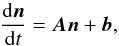 (A.1)where A is a matrix of coefficients, and b is a constant vector containing the artificial source terms that replenish dust in the parent belt16. This system of equations suffers from stiffness: the population levels of some bins change very rapidly compared to others mainly due to large differences in collisional timescales, and the time-step size is therefore determined by the stability of the integration method rather than by its accuracy. When using standard explicit integrators, this leads to an impractically small step size that prevents long integrations.
Following Löhne (2008), we resolve the stiffness by writing the differentials as  (A.2)where A′ is a diagonal matrix that contains only the diagonal elements of A, while the terms marked “const” contain the off-diagonal parts of A, as well as the constant terms b. Our integration scheme for the jth component of n, for timestep m + 1, reads as
![Mathematical equation: \appendix \setcounter{section}{1} \begin{equation} \label{eq:exp_eul} n_{ j, \; \! m + 1 } = n_{ j, \; \! m } \exp \left( A'_{ jk, \; \! m } \Delta t \right) + \frac{ \dot{n}_{ j, \; \! m }| \sub{const} }{ A'_{ jk, \; \! m } } \left[ \exp \left( A'_{ jk, \; \! m } \Delta t \right) - 1 \right], \end{equation}](/articles/aa/full_html/2014/11/aa22090-13/aa22090-13-eq310.png) (A.3)where Δt denotes the time-step size17. This scheme is known as the exponential Euler method (see Hochbruck & Ostermann 2010 for an introductory review). It is suitable for time integration of semi-linear problems, which consist of a stiff linear part and a non-stiff non-linear part. In short, the strategy is to solve the linear part exactly and to approximate the non-linear part using an explicit integration scheme.
(A.3)where Δt denotes the time-step size17. This scheme is known as the exponential Euler method (see Hochbruck & Ostermann 2010 for an introductory review). It is suitable for time integration of semi-linear problems, which consist of a stiff linear part and a non-stiff non-linear part. In short, the strategy is to solve the linear part exactly and to approximate the non-linear part using an explicit integration scheme.
The time-step size Δt is determined dynamically from the condition that population levels can never become negative. We use a scheme similar to that of Krivov et al. (2005), but adapted for the exponential Euler method.
Appendix A.2: Precalculation
Only considering collisions (i.e., ignoring diffusion terms), the evolution of the jth component of n can be written as (Löhne 2008)  (A.4)Here, t and p are the target and projectile bin indices, respectively, and Bjtp is an entry in the time-independent tensor of collisional coefficients B. Specifically, coefficient Bjtp is the rate at which the population level of bin j changes, per particle in bin t, per particle in bin p, combining all considered relative orbit orientations. If j = t or j = p, this is the loss rate of the target or projectile bin, respectively, caused by collisional destruction (assuming that the mass grid resolution is high enough that fragments do not end up in their parent bin). Otherwise, it is a rate at which fragments are created.
For the phase-space grids we use, the entire tensor B is too large to be stored in memory. However, it is very sparse, because (1) not all orbits that are part of the phase-space grid have mutual overlap; (2) overlap may occur for a limited range in relative orbit orientation; (3) impact velocities are not always high enough to cause catastrophic collisions; and (4) only a fraction of all possible masses are created as fragments.
By only storing the non-zero entries of B, it becomes possible to keep it in memory. We store the source and sink terms separately. For the source terms, which are by far the most memory intensive, each non-zero entry requires (1) the index of the target bin; (2) the index of the projectile bin; (3) the index of the bin fragment bin; and (4) the rate at which particles are created in the fragment bin, per particle in the target bin, per particle in the projectile bin. By further manual compression, only (3) and (4) need to be stored for each entry separately. The target bin index (1) only needs to be stored once for each possible target bin, along with the number of possible projectile bins for that target bin. Then, the projectile bin index (2) only needs to be stored once for each possible collisional pair of bins, along with the number of possible fragment bins for that pair. A similar scheme is used for the sink terms.
The compressed version of B is still very large (several gigabytes for the runs presented in this work). A disadvantage of the precalculation technique is therefore that the size of the grid that can be used is restricted by the available amount of memory, whereas a code that recalculates (parts of) B at each time step is only limited by CPU power. A cubic dependence of the non-zero entries of B on the number of mass bins (as opposed to quadratic dependencies on the orbital element variables) motivates the choice of a relatively small mass grid, representing only a part of the collisional cascade.
Appendix B: Model verification
We performed several tests to verify our numerical debris disk model. The P–R drag and sublimation modules of the code were tested by comparing the behavior of the model with independent numerical solutions of the equations of motion and sublimation for individual particles. For this purpose, the collisional module of the code was switched off, and a single bin was filled as the initial setup of the model, corresponding to the orbital elements of the particle. For all these tests, the resulting evolution of the dust distribution (not shown here) matches that of the independent solution. The accuracy of the predictions is limited by numerical diffusion and becomes better with higher resolution (i.e., larger phase-space grids).
To test the collisional module of our code, we benchmarked the model against the code of Krivov et al. (2006), by replicating one of their model runs for the debris disk of Vega as accurately as possible. Since the code of Krivov et al. (2006) uses semi-major axes as the distance dimension of the phase-space grid, the benchmark runs were performed with a version of our code that also uses the semi-major axis (as opposed to periastron distance, used in the rest of this paper). These runs do not include the effects of P–R drag or sublimation, so they can be used to separately test the collisional module of our code by switching off P–R drag and sublimation. Of the various runs presented by Krivov et al. (2006), the specific one that was reproduced is characterized by an initial optical depth profile in the outer disk (beyond 120 AU) that scales as τgeo(r) ∝ r-4, an initial eccentricity distribution between 0 and 0.375, and material properties for “rocky” grains. We refer the reader to Krivov et al. (2006) for the specific values used for parameters describing the phase-space grid, the initial setup of the disk, material properties, etc.
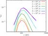 |
Fig. B.1 Evolution of the radial geometrical optical depth profile of the benchmark run, to be compared with Fig. 10 of Krivov et al. (2006). |
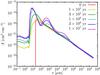 |
Fig. B.2 Evolution of the size distribution at r = 100 AU of the benchmark run, to be compared with Fig. 6 of Krivov et al. (2006). |
The evolution of the radial and size distribution predicted by the benchmark run are shown in Figs. B.1 and B.2, respectively. The corresponding results of Krivov et al. (2006) are their Figs. 10 and 6, respectively. Comparison of the results reveals good agreement between the two codes, and the remaining discrepancies can be accounted for. Relative to the benchmark, our model predicts (1) lower unbound particle populations and (2) shorter evolutionary timescales. Point (1) is to be expected since the unbound particle densities of Krivov et al. (2006) are computed using the product of their production rate and their disk crossing time, rather than from Eqs. (C.6) (Löhne, priv. comm.). We attribute point (2) to a mislabeling of the time steps in Figs. 6 and 10 of Krivov et al. (2006). Further discrepancies can be due to small differences in the input parameters and numerical techniques used.
Appendix C: Post-processing of model output
The output of a model run are the population levels n of all bins in the three-dimensional phase space of particle mass and orbital elements, as well as their change rates ṅ (which should equal zero once steady state is reached, except for bins corresponding to unbound orbits). While this data is useful for analyzing the orbital characteristics of different classes of particles in the debris disk, it is often more convenient to know about the state of the disk as a function of distance from the star. This is essential, for example, if the results of the model are to be compared with observations. Here, we describe the processing steps that are applied to the model output to derive the quantities used in Sect. 3.3.
Appendix C.1: Conversion from orbital elements to radial distance
To find the radial distribution of matter in the debris disk, the orbital element phase-space distribution function n(m,q,e) (dimension: [g-1 cm-1]) needs to be converted to the configuration space distribution function  , which denotes the vertically averaged number density of particles with masses [m,m + dm] at distance r (dimension: [g-1 cm-3]). This problem was first solved by Haug (1958) for a rotationally symmetric ensemble of particles on Keplerian orbits. Here, we give a brief derivation under the additional assumption that the distribution of inclinations is independent of the distribution of the other orbital elements.
Consider an individual particle on a bound Keplerian orbit that spends dt time to cross a radial annulus with width dr at distance r from the star. The contribution of this particle to is 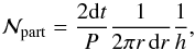 (C.1)where P is the particle’s orbital period, and h = 2r sin ε is the disk height, where ε is the semi-opening angle of the disk. The explicit factor 2 in the numerator accounts for the fact that the particle passes through this radial annulus twice during each orbit. In terms of orbital elements q and e, the orbital period P, accounting for direct radiation pressure, is given by
 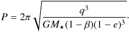 (C.2)The radial velocity ṙ of the particle is given by
 ![Mathematical equation: \appendix \setcounter{section}{3} \begin{equation} \label{eq:rdot} \frac{ \dif r }{ \dif t } = \pm \sqrt{ \frac{ G M\sub{\star} ( 1 - \beta ) }{r} \left[ 2 - \frac{r}{q} (1 - e) - \frac{q}{r} (1 + e) \right] }. \end{equation}](/articles/aa/full_html/2014/11/aa22090-13/aa22090-13-eq334.png) (C.3)Combining Eqs. (C.1)–(C.3), and considering all particles on bound orbits, gives (cf. Krivov et al. 2005)
(C.3)Combining Eqs. (C.1)–(C.3), and considering all particles on bound orbits, gives (cf. Krivov et al. 2005) ![Mathematical equation: \appendix \setcounter{section}{3} \begin{eqnarray} \label{eq:haug} \mathcal{N}(m,r) & = &\frac{1}{ 4 \pi^{2} \sin (\varepsilon) } \frac{1}{ r^{3} } \int\limits_{q} \! \! \! \int\limits_{e} n(m,q,e) \left[ \frac{r}{q} (1-e) \right]^{3/2} \nonumber\\ & &\quad \times \left[ 2 - \frac{r}{q}(1 - e) - \frac{q}{r}(1+e) \right]^{-1/2} \dif q \, \dif e, \end{eqnarray}](/articles/aa/full_html/2014/11/aa22090-13/aa22090-13-eq335.png) (C.4)with the integration domain
(C.4)with the integration domain 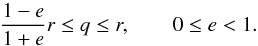 (C.5)The contribution of unbound particles to is calculated using their production rate ṅ(m,q,e) and the radial velocity with which they leave the system (Löhne, priv. comm.). Assuming all unbound particles are created at the periastron of their orbits, their vertically-averaged particle number density is given by
 ![Mathematical equation: \appendix \setcounter{section}{3} \begin{eqnarray} \label{eq:unbound_lohne_basic} \mathcal{N}(m,r) & = &\frac{ 1 }{ 2 \pi r h } \int\limits_{q} \! \! \! \int\limits_{e} \frac{ \dot n(m,q,e) }{ | \dot r(m,q,e,r) | } \, \dif q \, \dif e \\ \label{eq:unbound_lohne} & = & \frac{ 1 }{ 4 \pi \sin\varepsilon \sqrt{ G M\sub{\star} ( 1 - \beta ) r^3 } } \int\limits_{q} \! \! \! \int\limits_{e} \dot n(m,q,e) \nonumber\\ & &\quad \times \left[ 2 - \frac{r}{q} (1 - e) - \frac{q}{r} (1 + e) \right]^{-1/2} \dif q \, \dif e, \end{eqnarray}](/articles/aa/full_html/2014/11/aa22090-13/aa22090-13-eq338.png) with the integration domain
with the integration domain  (C.8)Negative eccentricities correspond to “anomalous” hyperbolic orbits (see Krivov et al. 2006).
In applying this theory to the raw data, we replace the integrals in Eqs. (C.4) and (C.7) with sums; replace n(m,q,e) and ṅ(m,q,e) with n and ṅ, respectively; and evaluate the resulting equations at discrete points of r. For each bin, we sample the phase space it represents using a Monte Carlo method.
Appendix C.2: Derived quantities
For radial dust distribution profiles, we use the vertical geometrical optical depth τgeo, defined as the surface density of collective (i.e., combining particles of all sizes) cross-section. It is computed from as  To characterize size distributions, we use the quantity A(s,r), defined as the cross-section density per base-10 logarithmic unit of size. It is given by
 ![Mathematical equation: \appendix \setcounter{section}{3} \begin{eqnarray} A(s,r) & = &\frac{ \dif s }{ \dif \log\sub{10} (s) } \frac{ \dif m }{ \dif s } \sigma(s) \mathcal{N}(m,r) \\[0.5em] & = &4 \pi^{2} \ln(10) \rho\sub{d} s^{5} \mathcal{N}(m,r). \end{eqnarray}](/articles/aa/full_html/2014/11/aa22090-13/aa22090-13-eq342.png) This quantity allows for an easy comparison between the relative contributions of particles with different sizes to the total cross-section of the disk. In the size distributions plots (Figs. 5 and 6), a horizontal line means particles of all sizes contribute equally to the cross-section, and equal areas under the curve correspond to equal contributions to the total cross-section.
This quantity allows for an easy comparison between the relative contributions of particles with different sizes to the total cross-section of the disk. In the size distributions plots (Figs. 5 and 6), a horizontal line means particles of all sizes contribute equally to the cross-section, and equal areas under the curve correspond to equal contributions to the total cross-section.
Kennedy & Wyatt (2013) find that “warm” exozodiacal dust around solar-type stars can be explained by in-situ planetesimal belts. This type of exozodiacal dust is detected at mid-infrared wavelengths and has a typical temperature of a few hundred K, placing it around 1 AU from the star.
The geometrical optical depth corresponds to the true vertical optical depth only for an extinction efficiency of unity (Qext = 1) for all particle sizes.
Assuming circular orbits is valid for particles with low β ratios, while the small particles most relevant to our study have high β ratios. We relax this simplifying assumption in our numerical model (Sect. 3).
Equation (3) ignores a factor  in the orbital period of radiation pressure affected particles, but this only changes the collisional timescale by a factor of about 0.7 for β = 0.5.
Debris disks around stars with a strong stellar wind have higher values of τgeo. We ignore stellar wind in our present analysis, and discuss its effects in Sect. 5.2.
While larger grains constitute more mass for a given geometrical optical depth profile (m/τgeo ∝ m/σ ∝ s), they also migrate more slowly (ṙPR ∝ β ∝ s-1). These two effects cancel each other out.
Following Wien’s displacement law, λ⋆ ≈ 0.5 μm for the stars considered in this research.
More precise estimates of the pile-up distance are given by Kobayashi et al. (2009, 2011). We use this simple approximation to facilitate the estimate of the pile-up magnitude in Sect. 2.3.2.
Integrating over true anomaly rather than, e.g., mean anomaly warrants a higher sampling around the periastron, where sublimation rate varies the most.
If the radial geometrical optical depth is higher than ~10-2, the disk is subject to dust avalanches (Grigorieva et al. 2007).
The actual input parameter used (which indirectly determines the geometrical optical depth at the source region) is the mass supply term of large dust particles in the source region (see Sect. 3.2.4). It is set to 10-10M⊕yr-1 for the M⋆ = 1 M⊙ run and 8 × 10⁻¹⁰M⊕yr-1 for the M⋆ = 2 M⊙ run. Comparing these mass fluxes to those given by Eq. (11) indicates that the vast majority of the material is destroyed in collisions before it reaches the sublimation zone.
Formally, steady state is only reached after ~ 10 Gyr, which is the time it takes for the largest particles we consider to move from the parent belt to the sublimation zone by P–R drag. The barely bound grains that dominate the cross-section, however, already settle into a steady state after ~ 10 Myr, which is short compared to the typical lifetime of a debris disk.
Our approach to computing the SED of a dust profile with pile-up is different from that of Kobayashi et al. (2011), who use τgeo, pile and Δrpile as independent input variables. In our estimate, the total amount of dust is fixed, and placing it all at rpile is the most optimistic configuration for detecting the pile-up.
In debris disks relative velocities are mostly due to the eccentricities and mutual inclinations of particle orbits. While orbital eccentricities are diminished in the inner disk by P–R drag induced circularization, inclinations are simply inherited from the parent belt. This is handled correctly in our code, since orbital inclinations are parameterized by the (constant) opening angle of the disk.
For the M⋆ = 1 M⊙, r0 = 30 AU case, the pile-up efficiency should be at least ~100 times higher to make the slope of the SED negative.
Collision rates are proportional to target and projectile densities, so the entries of matrix A contain terms with elements of n. Because target and projectile bin can be the same, the system of equations is in fact non-linear.
This corresponds to Eq. (3.107) of Löhne (2008), corrected for a typographical error.
Acknowledgments
We thank the anonymous referee for a very thorough and detailed report, that helped us to improve the quality of this paper.
References
- Abrahamson, J. 1974, Carbon, 12, 111 [CrossRef] [Google Scholar]
- Absil, O., di Folco, E., Mérand, A., et al. 2006, A&A, 452, 237 [NASA ADS] [CrossRef] [EDP Sciences] [Google Scholar]
- Absil, O., di Folco, E., Mérand, A., et al. 2008, A&A, 487, 1041 [NASA ADS] [CrossRef] [EDP Sciences] [Google Scholar]
- Absil, O., Mennesson, B., Le Bouquin, J.-B., et al. 2009, ApJ, 704, 150 [NASA ADS] [CrossRef] [Google Scholar]
- Absil, O., Defrère, D., Coudé du Foresto, V., et al. 2013, A&A, 555, A104 [NASA ADS] [CrossRef] [EDP Sciences] [Google Scholar]
- Acke, B., Min, M., Dominik, C., et al. 2012, A&A, 540, A125 [NASA ADS] [CrossRef] [EDP Sciences] [Google Scholar]
- Akeson, R. L., Ciardi, D. R., Millan-Gabet, R., et al. 2009, ApJ, 691, 1896 [NASA ADS] [CrossRef] [Google Scholar]
- Allen, C. W. 1976, Astrophysical Quantities (London: Athlone) [Google Scholar]
- Babel, J. 1995, A&A, 301, 823 [Google Scholar]
- Backman, D. E., & Paresce, F. 1993, in Protostars and Planets III, eds. E. H. Levy, & J. I. Lunine, 1253 [Google Scholar]
- Benz, W., & Asphaug, E. 1999, Icarus, 142, 5 [NASA ADS] [CrossRef] [Google Scholar]
- Bonsor, A., Augereau, J.-C., & Thébault, P. 2012, A&A, 548, A104 [NASA ADS] [CrossRef] [EDP Sciences] [Google Scholar]
- Bonsor, A., Kennedy, G. M., Crepp, J. R., et al. 2013, MNRAS, 431, 3025 [NASA ADS] [CrossRef] [Google Scholar]
- Burns, J. A., Lamy, P. L., & Soter, S. 1979, Icarus, 40, 1 [NASA ADS] [CrossRef] [Google Scholar]
- Campo Bagatin, A., Cellino, A., Davis, D. R., Farinella, P., & Paolicchi, P. 1994, Planet. Space Sci., 42, 1079 [NASA ADS] [CrossRef] [Google Scholar]
- Carpenter, J. M., Bouwman, J., Mamajek, E. E., et al. 2009, ApJS, 181, 197 [NASA ADS] [CrossRef] [Google Scholar]
- Chen, C. H., Patten, B. M., Werner, M. W., et al. 2005, ApJ, 634, 1372 [NASA ADS] [CrossRef] [Google Scholar]
- Chen, C. H., Sargent, B. A., Bohac, C., et al. 2006, ApJS, 166, 351 [NASA ADS] [CrossRef] [Google Scholar]
- Ciardi, D. R., van Belle, G. T., Akeson, R. L., et al. 2001, ApJ, 559, 1147 [NASA ADS] [CrossRef] [Google Scholar]
- Defrère, D., Absil, O., Augereau, J.-C., et al. 2011, A&A, 534, A5 [NASA ADS] [CrossRef] [EDP Sciences] [Google Scholar]
- Defrère, D., Lebreton, J., Le Bouquin, J.-B., et al. 2012, A&A, 546, L9 [NASA ADS] [CrossRef] [EDP Sciences] [Google Scholar]
- Dent, W. R. F., Walker, H. J., Holland, W. S., & Greaves, J. S. 2000, MNRAS, 314, 702 [NASA ADS] [CrossRef] [Google Scholar]
- di Folco, E., Thévenin, F., Kervella, P., et al. 2004, A&A, 426, 601 [NASA ADS] [CrossRef] [EDP Sciences] [Google Scholar]
- di Folco, E., Absil, O., Augereau, J.-C., et al. 2007, A&A, 475, 243 [NASA ADS] [CrossRef] [EDP Sciences] [Google Scholar]
- Dohnanyi, J. S. 1969, J. Geophys. Res., 74, 2531 [NASA ADS] [CrossRef] [Google Scholar]
- Dominik, C., & Decin, G. 2003, ApJ, 598, 626 [NASA ADS] [CrossRef] [Google Scholar]
- Durda, D. D., & Dermott, S. F. 1997, Icarus, 130, 140 [NASA ADS] [CrossRef] [Google Scholar]
- Eiroa, C., Marshall, J. P., Mora, A., et al. 2013, A&A, 555, A11 [NASA ADS] [CrossRef] [EDP Sciences] [Google Scholar]
- Flynn, G. J., & Durda, D. D. 2004, Planet. Space Sci., 52, 1129 [CrossRef] [Google Scholar]
- Fujiwara, A., Kamimoto, G., & Tsukamoto, A. 1977, Icarus, 31, 277 [NASA ADS] [CrossRef] [Google Scholar]
- Gáspár, A., Psaltis, D., Rieke, G. H., & Özel, F. 2012, ApJ, 754, 74 [NASA ADS] [CrossRef] [Google Scholar]
- Gáspár, A., Rieke, G. H., & Balog, Z. 2013, ApJ, 768, 25 [NASA ADS] [CrossRef] [Google Scholar]
- Greaves, J. S., Wyatt, M. C., Holland, W. S., & Dent, W. R. F. 2004, MNRAS, 351, L54 [NASA ADS] [CrossRef] [MathSciNet] [Google Scholar]
- Grigorieva, A., Artymowicz, P., & Thébault, P. 2007, A&A, 461, 537 [NASA ADS] [CrossRef] [EDP Sciences] [Google Scholar]
- Haug, U. 1958, Z. Astrophys., 44, 71 [NASA ADS] [Google Scholar]
- Heng, K., & Tremaine, S. 2010, MNRAS, 401, 867 [NASA ADS] [CrossRef] [Google Scholar]
- Hochbruck, M., & Ostermann, A. 2010, Acta Numerica, 19, 209 [Google Scholar]
- Hollis, J. M., Chin, G., & Brown, R. L. 1985, ApJ, 294, 646 [NASA ADS] [CrossRef] [Google Scholar]
- Kalas, P., Graham, J. R., & Clampin, M. 2005, Nature, 435, 1067 [NASA ADS] [CrossRef] [PubMed] [Google Scholar]
- Kennedy, G. M., & Wyatt, M. C. 2013, MNRAS, 433, 2334 [NASA ADS] [CrossRef] [Google Scholar]
- Kobayashi, H., Watanabe, S.-I., Kimura, H., & Yamamoto, T. 2008, Icarus, 195, 871 [NASA ADS] [CrossRef] [Google Scholar]
- Kobayashi, H., Watanabe, S.-I., Kimura, H., & Yamamoto, T. 2009, Icarus, 201, 395 [NASA ADS] [CrossRef] [Google Scholar]
- Kobayashi, H., Kimura, H., Watanabe, S.-i., Yamamoto, T., & Müller, S. 2011, Earth, Planets, and Space, 63, 1067 [Google Scholar]
- Krivov, A. V., Sremčević, M., & Spahn, F. 2005, Icarus, 174, 105 [NASA ADS] [CrossRef] [Google Scholar]
- Krivov, A. V., Löhne, T., & Sremčević, M. 2006, A&A, 455, 509 [NASA ADS] [CrossRef] [EDP Sciences] [Google Scholar]
- Lagage, P. O., & Pantin, E. 1994, Nature, 369, 628 [NASA ADS] [CrossRef] [Google Scholar]
- Lawler, S. M., Beichman, C. A., Bryden, G., et al. 2009, ApJ, 705, 89 [NASA ADS] [CrossRef] [Google Scholar]
- Lebreton, J., van Lieshout, R., Augereau, J.-C., et al. 2013, A&A, 555, A146 [NASA ADS] [CrossRef] [EDP Sciences] [Google Scholar]
- Löhne. 2008, Ph.D. Thesis, Friedrich-Schiller-Universität Jena, Germany [Google Scholar]
- Marshall, J. P., Krivov, A. V., del Burgo, C., et al. 2013, A&A, 557, A58 [NASA ADS] [CrossRef] [EDP Sciences] [Google Scholar]
- Mennesson, B., Absil, O., Lebreton, J., et al. 2013, ApJ, 763, 119 [NASA ADS] [CrossRef] [Google Scholar]
- Min, M., Hovenier, J. W., & de Koter, A. 2005, A&A, 432, 909 [NASA ADS] [CrossRef] [EDP Sciences] [Google Scholar]
- Minato, T., Köhler, M., Kimura, H., Mann, I., & Yamamoto, T. 2004, A&A, 424, L13 [NASA ADS] [CrossRef] [EDP Sciences] [Google Scholar]
- Minato, T., Köhler, M., Kimura, H., Mann, I., & Yamamoto, T. 2006, A&A, 452, 701 [NASA ADS] [CrossRef] [EDP Sciences] [Google Scholar]
- Morales, F. Y., Werner, M. W., Bryden, G., et al. 2009, ApJ, 699, 1067 [NASA ADS] [CrossRef] [Google Scholar]
- Pantin, E., Lagage, P. O., & Artymowicz, P. 1997, A&A, 327, 1123 [NASA ADS] [Google Scholar]
- Plavchan, P., Werner, M. W., Chen, C. H., et al. 2009, ApJ, 698, 1068 [NASA ADS] [CrossRef] [Google Scholar]
- Preibisch, T., Ossenkopf, V., Yorke, H. W., & Henning, T. 1993, A&A, 279, 577 [NASA ADS] [Google Scholar]
- Rafikov, R. R. 2011, ApJ, 732, L3 [NASA ADS] [CrossRef] [Google Scholar]
- Reidemeister, M., Krivov, A. V., Stark, C. C., et al. 2011, A&A, 527, A57 [NASA ADS] [CrossRef] [EDP Sciences] [Google Scholar]
- Strubbe, L. E., & Chiang, E. I. 2006, ApJ, 648, 652 [NASA ADS] [CrossRef] [Google Scholar]
- Su, K. Y. L., Rieke, G. H., Malhotra, R., et al. 2013, ApJ, 763, 118 [NASA ADS] [CrossRef] [Google Scholar]
- Takeuchi, T., & Artymowicz, P. 2001, ApJ, 557, 990 [NASA ADS] [CrossRef] [Google Scholar]
- Thébault, P., & Augereau, J.-C. 2007, A&A, 472, 169 [NASA ADS] [CrossRef] [EDP Sciences] [Google Scholar]
- Trilling, D. E., Bryden, G., Beichman, C. A., et al. 2008, ApJ, 674, 1086 [NASA ADS] [CrossRef] [Google Scholar]
- Vitense, C., Krivov, A. V., & Löhne, T. 2010, A&A, 520, A32 [NASA ADS] [CrossRef] [EDP Sciences] [Google Scholar]
- Wyatt, M. C. 2005, A&A, 433, 1007 [NASA ADS] [CrossRef] [EDP Sciences] [Google Scholar]
- Wyatt, M. C. 2008, ARA&A, 46, 339 [NASA ADS] [CrossRef] [Google Scholar]
- Wyatt, M. C., Smith, R., Greaves, J. S., et al. 2007, ApJ, 658, 569 [NASA ADS] [CrossRef] [Google Scholar]
- Wyatt, S. P., & Whipple, F. L. 1950, ApJ, 111, 134 [NASA ADS] [CrossRef] [Google Scholar]
- Zavitsanos, P. D., & Carlson, G. A. 1973, J. Chem. Phys., 59, 2966 [NASA ADS] [CrossRef] [Google Scholar]
All Tables
NIR interferometric detections of hot exozodiacal dust, together with associated outer debris belt locations.
All Figures
|
Fig. 1 Maximum geometrical optical depth as a function of distance to the star (Eq. (5)). The profiles are derived from the analytical model of Wyatt (2005), in which dust is produced by a source at radius r0 and subsequently migrates inward due to P–R drag, while suffering destruction from mutual collisions. The solid lines correspond to solar-mass stars, the dashed lines to 2 M⊙ stars. Profiles for different parent belt locations are shown in different colors. All profiles assume dust grains with β = 0.5. |
| In the text | |
|
Fig. 2 Characteristic timescale as function of radial distance for sublimation (Eq. (15)), P–R drag (Eq. (2)), and mutual collisions (minimum timescale, Eq. (23)), for β = 0.5 particles in a debris disk around a solar-mass star with a very dense (η0 ≫ 1) parent belt located at 30 AU. The gray vertical lines indicate the radial distances used by the analytical model: rpile is the radius for which the sublimation timescale equals the P–R drag timescale, rcrit is the radius for which the P–R drag timescale equals the collisional timescale, and r0 is the location of the parent belt. For the sublimation timescale, we assume that the dust grains are solid spheres of graphite (see Sect. 2.2.1 for the values of the sublimation parameters) with a radius of s = 0.64 μm (the size corresponding to β = 0.5). |
| In the text | |
|
Fig. 3 Maximum geometrical optical depth profiles of debris disks with collisions, P–R drag, and sublimation (Eq. (28) with τgeo, base(r) given by Eq. (5)), for different values of relative pile-up width Δrpile/rpile shown in different colors. The solid lines correspond to disks around solar-mass stars, the dashed lines to disks around 2 M⊙ stars. All profiles assume a parent belt at r0 = 30 AU, dust grains with β = 0.5, and rpile ≈ 0.019 AU, and rpile ≈ 0.064 AU, for the M⋆ = 1 M⊙, and M⋆ = 2 M⊙ cases, respectively, corresponding to spherical graphite grains with β = 0.5. |
| In the text | |
|
Fig. 4 Geometrical optical depth profiles of debris disks with a dense parent belt at 30 AU around stars of M⋆ = 1 M⊙ (solid lines) and M⋆ = 2 M⊙ (dashed lines). The black lines show the end results of the numerical simulations. In green are the maximum τgeo profiles as given by the analytical model (Eq. (28), with τgeo, base(r) given by Eq. (5), Δrpile/rpile = 0.15, r0 = 30 AU, and β = 0.5). |
| In the text | |
|
Fig. 5 Size distributions at different radial distances for the M⋆ = 1 M⊙ run before switching on sublimation. The quantity on the vertical axis, A, is the cross-section density per unit size decade (see Appendix C.2), which is horizontal if all sizes contribute equally to the cross-section. The gray band indicates the slope of a size distribution that follows the classical Dohnanyi (1969) power law (n(s) ∝ s-3.5, hence A ∝ s-0.5). The vertical lines mark the particle sizes corresponding to relevant values of β. |
| In the text | |
|
Fig. 6 Size distribution at r = 0.02 AU (the location of pile-up) for the M⋆ = 1 M⊙ run, before and after sublimation is switched on. |
| In the text | |
|
Fig. 7 SEDs of stars and their debris disks at a distance of 10 pc. The disk SED is shown for different dust distributions with the numerical results in black and the analytical distributions in green. Dust distributions including the pile-up of dust in the sublimation zone are shown with dashed lines, and distributions in which the pile-up is excluded are shown with solid lines, but the spectra largely overlap. Disk SEDs are calculated according to Eqs. (46) and (47). The stellar photosphere is indicated by a dotted Planck curve. The vertical gray areas mark the NIR H and K bands in which hot exozodiacal dust is observed. |
| In the text | |
|
Fig. 8 Flux ratio between the disk and the star at 2.1 μm (K band), as function of parent belt radius r0. Solid lines indicate the flux ratio due to the maximum amount of material moved in by P–R drag, truncated at r = rpile. Ratios including the small effect due to pile-up are shown with dashed lines. Different colors are used for different stellar types. The light shaded area marks the region in parameter space where no significant pile-up is expected to occur because the orbits of small dust grains cannot circularize sufficiently (see Eq. (22)). The dark shaded area marks where the parent belt r0 is closer than the pile-up radius rpile. The observed K-band excess fluxes of main-sequence stars from Table 1 are shown at their respective estimated parent belt distances with a different symbol for each star and coloring according to the star’s spectral type: Vega (the CHARA/FLUOR measurement): circles; β Leo: hexagon; Fomalhaut: squares; β Pic: diamond; η Lep: upward pointing triangles; 110 Her: left-pointing triangle; 10 Tau: right-pointing triangle; τ Cet: pentagon. |
| In the text | |
|
Fig. B.1 Evolution of the radial geometrical optical depth profile of the benchmark run, to be compared with Fig. 10 of Krivov et al. (2006). |
| In the text | |
|
Fig. B.2 Evolution of the size distribution at r = 100 AU of the benchmark run, to be compared with Fig. 6 of Krivov et al. (2006). |
| In the text | |
Current usage metrics show cumulative count of Article Views (full-text article views including HTML views, PDF and ePub downloads, according to the available data) and Abstracts Views on Vision4Press platform.
Data correspond to usage on the plateform after 2015. The current usage metrics is available 48-96 hours after online publication and is updated daily on week days.
Initial download of the metrics may take a while.