| Issue |
A&A
Volume 626, June 2019
|
|
|---|---|---|
| Article Number | A2 | |
| Number of page(s) | 19 | |
| Section | Interstellar and circumstellar matter | |
| DOI | https://doi.org/10.1051/0004-6361/201935250 | |
| Published online | 30 May 2019 | |
Hot exozodiacal dust: an exocometary origin?
1
CNRS, IPAG, Université Grenoble Alpes,
38000
Grenoble, France
e-mail: This email address is being protected from spambots. You need JavaScript enabled to view it.
2
LESIA, Observatoire de Paris, CNRS, Université Paris Diderot, Université Pierre et Marie Curie,
5 place Jules Janssen,
92190
Meudon,
France
Received:
11
February
2019
Accepted:
12
March
2019
Abstract
Context. Near- and mid-infrared interferometric observations have revealed populations of hot and warm dust grains populating the inner regions of extrasolar planetary systems. These are known as exozodiacal dust clouds, or exozodis, reflecting the similarity with the solar system’s zodiacal cloud. Radiative transfer models have constrained the dust to be dominated by tiny submicron-sized, carbon-rich grains that are accumulated very close to the sublimation radius. The origin of this dust is an unsolved issue.
Aims. We explore two exozodiacal dust production mechanisms, first re-investigating the Poynting-Robertson drag pile-up scenario, and then elaborating on the less explored but promising exocometary dust delivery scenario.
Methods. We developed a new, versatile numerical model that calculates the dust dynamics, with non-orbit-averaged equations for the grains close to the star. The model includes dust sublimation and incorporates a radiative transfer code for direct comparison to the observations. We consider in this study four stellar types, three dust compositions, and we assume a parent belt at 50 au.
Results. In the case of the Poynting-Robertson drag pile-up scenario, we find that it is impossible to produce long-lived submicron-sized grains close to the star. The inward drifting grains fill in the region between the parent belt and the sublimation distance, producing an unrealistically strong mid-infrared excess compared to the near-infrared excess. The dust pile-up at the sublimation radius is by far insufficient to boost the near-IR flux of the exozodi to the point where it dominates over the mid-infrared excess. In the case of the exocometary dust delivery scenario, we find that a narrow ring can form close to the sublimation zone, populated with large grains from several tens to several hundreds of micrometers in radius. Although not perfect, this scenario provides a better match to the observations, especially if the grains are carbon-rich. We also find that the number of active exocomets required to sustain the observed dust level is reasonable.
Conclusions. We conclude that the hot exozodiacal dust detected by near-infrared interferometry is unlikely to result from inward grain migration by Poynting-Robertson drag from a distant parent belt, but could instead have an exocometary origin.
Key words: zodiacal dust / circumstellar matter / methods: numerical / infrared: planetary systems / comets: general
© É. Sezestre et al. 2019
 Open Access article, published by EDP Sciences, under the terms of the Creative Commons Attribution License (http://creativecommons.org/licenses/by/4.0), which permits unrestricted use, distribution, and reproduction in any medium, provided the original work is properly cited.
1 Introduction
Hot exozodiacal dust clouds (exozodis) have been detected by means of interferometric observations in the near-infrared (near-IR, H- or K-band), around about 25 main sequence stars (Absil et al. 2013; Ertel et al. 2014, 2016; Kral et al. 2017; Nuñez et al. 2017). These exozodis are very bright, amounting to ~1% of the stellar flux in the K-band, which is about 1000 times more than the solar system’s own zodiacal cloud in the same spectral range. For some of these systems, a warm counterpart has also been detected in the mid-infrared (mid-IR, 8–20 μm, e.g., Mennesson et al. 2013, 2014; Su et al. 2013; Ertel et al. 2018), but this mid-IR exozodi-to-star flux ratio never exceeds the flux ratios in the H- or K-band (Kirchschlager et al. 2017). Furthermore, for the handful of systems for which parametric modeling based on radiative transfer codes has been performed (Absil et al. 2006, 2008; Di Folco et al. 2007; Akeson et al. 2009; Defrère et al. 2011; Lebreton et al. 2013; Kirchschlager et al. 2017), the ratio between the fluxes in the near-IR and mid-IR has constrained the dust to be dominated by tiny submicron-sized grains that are accumulated very close to the sublimation radius rs (typically a few stellar radii).
The presence of such large amounts of very small grains so close to their star poses a challenge when it comes to explaining the origin of the exozodis. The canonical explanation invoked for standard cold debris disks, i.e., the in situ steady production of small grains by a collisional cascade starting from larger parent bodies (e.g., Krivov 2010), cannot hold here because collisional erosion is much too fast in these innermost regions to be sustained over periods comparable to the system’s age (Bonsor et al. 2012; Kral et al. 2017). Therefore, the long-term existence of a hot exozodi requires both an external reservoir of material and an inward transport mechanism, feeding with dust the region close to the sublimation radius at a rate of about 10−10–10−9 M⊕ yr−1 (e.g., Absil et al. 2006; Kral et al. 2017). A significant fraction (more than ~20%) of nearby solar- and A-type stars possess an extrasolar analog to the Kuiper belt (Montesinos et al. 2016; Sibthorpe et al. 2018; Thureau et al. 2014), indicating that external reservoirs for exozodis are common. The inward transport mechanism must then be sufficiently generic to affect more than 10% of the nearby stars, independent of their age and spectral type (Ertel et al. 2014; Nuñez et al. 2017). For instance, large-scale dynamical instabilities in planetary systems, that could occur randomly (e.g., the Late Heavy Bombardment in the solar system), were shown to significantly increase the number of small bodies scattered from an external Kuiper-like belt toward the star, but because each event lasts less than a few million years, the probability of observing hot exozodiacal dust produced during such an event is less than 0.1% (Bonsor et al. 2013). This mechanism cannot explain the vast majority of the hot exozodis.
To date, two main categories of exozodi-origin scenarios have been explored. The first assumes that the dust is collisionally produced farther out in the system (in an asteroidal or Kuiper-like belt) and migrates inward because of Poynting-Robertson drag (hereafter PR-drag), until it reaches the sublimation distance rs. There, it starts to sublimate and shrink until radiation pressure becomes significant and increases its orbital semi-major axis and eccentricity, while keeping its periastron nearly the same. This will slow down the inward migration and thus potentially create a pile-up of small grains close to rs. This scenario follows the pioneering work of Belton (1966) predicting a density peak near the sublimation distance in the solar system, and the works by Mukai et al. (1974) and Mukai & Yamamoto (1979) attempting to explain the observed flux bump at about 4 R⊙ in the F-corona (the hot component of the zodiacal dust cloud). However, the estimated amplitude of this pile-up seems to be too weak to explain the observed near-IR excesses in extrasolar systems (Kobayashi et al. 2008, 2009, 2011; Van Lieshout et al. 2014). Another problem is that this scenario does not seem to be able to produce grains that are as small as those derived from radiative transfer modeling. However, it is worth noting that these results were obtained using orbit-averaged equations of motion that might become inaccurate close to rs because of the very fast variations imposed by the sublimation.
A second way of delivering dust in the innermost regions of planetary systems is by the sublimation of large asteroidal or cometary bodies, originating in an external belt, and scattered inward by a chain of low-mass planets (Bonsor et al. 2012, 2014; Raymond & Bonsor 2014; Marboeuf et al. 2016). There is evidence for exocometary activity around other stars than the Sun, found through the observation of transient, Doppler-shifted gas absorption lines (e.g., Beust & Morbidelli 2000; Kiefer et al. 2014a,b, and references therein), and the analysis of Kepler transit light curves attributed to trailing dust tails passing in front of the star (Kiefer et al. 2017; Rappaport et al. 2018, with mass loss rates of ~ 10−12 and > 10−10 M⊕ yr−1, respectively). In the solar system, comets are supposed to contribute significantly to the zodiacal cloud (e.g., Liou et al. 1995; Dermott et al. 1996). Nesvorný et al. (2010) estimated for example that ~ 90% of the zodiacal dust originates from Jupiter family comets. The cometary hypothesis as a source of hot exozodiacal dust has, however, never been tested quantitatively in terms of the level of dustiness that can be obtained near the rs region.
This paper reinvestigates both these scenarios. For the PR-drag case (Sect. 3), we use for the first time a sophisticated numerical model that does not rely on orbit-averaged equations in the crucial sublimation region (Sect. 2). We also explore the potential role played by the differential Doppler effect (DDE) evoked by Kimura et al. (2017, 10th Meeting on Cosmic Dust, Tokyo)1. As for the comet-delivery case, we perform the first quantitative exploration of this scenario in the context of exozodis, following the fate of the dust that is produced as the comet sublimates (Sect. 4). For each scenario, we explore a wide range of possible grain compositions and stellar types (Sect. 2). Rather than checking the validity of each scenario by assessing how well they can reproduce the predictions of radiative-model fits (grain location and typical sizes), we chose to directly focus on the observational constraints themselves, in particular the fluxes in the near- and mid-IR.
2 Numerical model
2.1 General philosophy
We use in essence the same numerical code to investigate both the PR-drag pile-up and the cometary delivery scenarios. Our model performs a consistent treatment of a grain’s evolution, from its release to its ejection, sublimation, or fall onto the star. We take into account stellar gravity, stellar radiation/wind pressure, PR-drag, and sublimation. In a more advanced version, the stellar magnetic field can be turned on, but this capability will not be used in this paper.
In this study, we chose to neglect collective effects such as mutual collisions. This might appear as a step back when compared to the studies of Kobayashi et al. (2009) and Van Lieshout et al. (2014), who did take into account collisional effects (albeit in a very simplified way) for the PR-drag pile-up scenario. However, we believe that this neglect of collisions does not radically bias our results. Van Lieshout et al. (2014) has indeed shown that, because of the self-regulating interplay between collisions and PR-drag, collisional effects will only play a significant role, potentially halting the inward drift of grains, very close to the location of the parent body belt releasing the dust grains. As soon as the dust has migrated away from the parent belt, its number density is always low enough for mutual collisions not to have a major effect on its evolution (see Fig. 2 in Van Lieshout et al. 2014). In this respect, the only drawback of not taking into account collisions is that we cannot derive the density and the mass of the dust-producing parent belt, but this is not the main focus of our study, which concentrates on the evolution of the dust once it has reached the inner regions of the system.
For the dust evolution in these innermost regions, our code presents a step forward compared to previous studies because it does not rely on orbit-averaged da/dt and de/dt estimates, but integrates the exact equations of motion up until the grain is removed. This is a crucial point in the critical region close to the sublimation radius, where a grain radius can vary on timescales much smaller than the local orbital period, thus inducing dynamical changes that cannot be accounted for with averaged estimates. In addition, the orbit-averaged de/dt estimates can lead to eccentricity values that can be infinitely small, whereas in reality there is always a minimum “residual” osculating eccentricity below which the particle’s orbit cannot go (see Sect. 3.1).
In addition to the dust evolution, the output of the code is a global density map assuming the system is at steady state. This is used to produce a synthetic spectrum of the exozodi that can be compared to measured spectra, and also flux levels measured by interferometric studies. Since the mass of dust close to the star in the PR-drag scenario is not constrained by the mass of the dust producing belt, we try to reproduce the trend of the spectra, and use the mass of the exozodi as a free parameter. More specifically, we scale the mass such that the excess corresponds to observationsat 2 μm, and we use the excess observed in mid-IR to discuss the relevancy of the examined scenarios (around 1% at 8–20 μm; e.g., Kirchschlager et al. 2017). On the contrary, in the cometary release scenario, the flux level can be estimated by the mass of the releasing comet, providing constraints on its radius.
2.2 Dynamical approach
The code computes the dynamics of a set of compact dust grains with initial sizes chosen to sample different dynamical behaviors. The equation of motion is solved with a fourth-order Runge-Kutta integrator with an adaptive timestep. The code is able to take into account stellar gravity (Fgrav), radiation pressure and Poynting-Roberston drag (FPR), and differential Doppler effect (FDDE; e.g., Burns et al. 1979). Each of these effects can be individually switched on or off at any time.
The forces are expressed as
![Mathematical equation: \begin{eqnarray}&& \hspace*{-6pt}{\boldsymbol F}_{\textrm{grav}} = - \frac{G M_{\star} m }{r^2} \cdot \vec{e}_{\textrm{r}},\\ && \hspace*{-6pt}{\boldsymbol F}_{\textrm{PR}} = \beta_{\textrm{pr}} \frac{G M_{\star} m }{r^2} \> \left[ \left( 1 - \frac{\dot{r}}{c} \right) \vec{e}_{\textrm{r}} - \frac{{\boldsymbol v}}{c} \right],\\ && \hspace*{-6pt}{\boldsymbol F}_{\textrm{DDE}} = - \frac{\omega_{\star} R_{\star}^2 }{4} \frac{\beta_{\textrm{pr}}}{\sqrt{1-\beta_{\textrm{pr}}} } \sqrt{\frac{GM_{\star}}{r^5}} \cdot \frac{{\boldsymbol v}}{c},\end{eqnarray}](/articles/aa/full_html/2019/06/aa35250-19/aa35250-19-eq1.png)
where er is the radial unit vector, G the gravitational constant, c the speed of light, M⋆ the mass of the star, R⋆ the stellar radius, ω⋆ the rotation frequency of the star, m the mass of the grain, r the distance of the grain to the star, v the grain velocity and ṙ the radial velocity, and βpr the ratio of the radiation pressure force to the gravitational force.
Other forces, in particular the stellar wind pressure and the Lorentz force, are implemented in the code but will not be used in this study. The pressure due to the stellar wind is comparable to the radiation pressure alone for submicron-sized grains around late-type stars. As we focus on K-type and earlier stars (Sect. 2.3), we do not take into account the stellar wind pressure. For consistency and simplicity, we refer to the βpr parameter as β in the following. The Lorentz force acting on charged grains interacting with the large-scale stellar magnetic field can also affect the grain dynamics, as evidenced by Czechowski & Mann (2012) and Rieke et al. (2016). We will also not discuss the Lorentz force as it is beyond the scope of this study.
The initial conditions of the simulations depend on the scenario that is considered. These are detailled in Sects. 3 and 4 for the PR-drag pile-up and the cometary delivery scenarios, respectively. The grain dynamics is computed until one of following criteria is met:
-
the grain sublimates completely. This occurs when the grain size is below the lower limit of the predefined size grid, which in most cases corresponds to a size smaller than 1 nm;
-
the grain falls onto the star. This is assumed to happen when the distance of the grain to the surface of the star is less than 0.1 R⋆;
-
the grain is expelled. This is assumed to occur when the distance to the star is over 1000 au;
-
the grain is too old. This is considered to be the case when the integration time is over one million years, meaning the grain has not evolved.
The integration timestep is taken as a fraction of the local revolution period (typically a hundredth), to ensure a sufficient resolution at every distance from the star. As a test of the code, we reproduced the results in Fig. 5 of Krivov et al. (1998) with great precision, as shown in Fig. A.1. However, for the grains released from parent bodies in a distant belt and then migrating inward by PR-drag, like in the scenario developed in Sect. 3, this short timestep becomes a numerical limitation. Therefore, and as long as the grain remains far from the star, we opt in this case for the orbit-averaged prescription of Wyatt & Whipple (1950, their Eq. (9)) to evolve the grains by PR-drag. This approach saves computational time during the less critical evolution stages (stage I as defined in Sect. 3.1.1), and is similar to the methodology employed by Kobayashi et al. (2009) and Van Lieshout et al. (2014). According to Wyatt & Whipple (1950), the quantity ae−4∕5(1 − e2) remains constant during the PR-dragmigration, where a is the grain semi-major axis and e its eccentricity. We use this conservation principle to estimate the semi-major axis and the eccentricity as the grain migrates inward until the full, non-orbit-averaged simulation is switched on, in contrast with what was done in previous studies. The switch is done when the grain reaches an equilibrium temperature at periastron that is half its sublimation temperature, to prevent sublimation from occurring during the orbit-averaged phase. We also continuously monitor the evolution of the grain radius due to sublimation during this phase in order to stop the orbit-averaged treatment if the radius is decreased by more than 1% of its initial value. We checked on a test run that this approach provides the same results as those obtained with the full simulation. In the cometary scenario developed in Sect. 4, it should be noted that the whole grain evolution was done using non-orbit-averaged equations.
Reference stars used in the code.
2.3 Stellar and grain properties
In this paper, we consider four different stellar types, ranging from A0 to K0. For this purpose, we chose four representative nearby starsthat do not necessarily possess hot exozodiacal dust. Their properties are summarized in Table 1.
We consider three different grain compositions, parameterized by their physical, optical, and thermodynamical properties. In the following, “carbon” refers to amorphous carbonaceous grains, “astrosilicates” and “glassy silicate” to amorphous silicate grains. The two silicate compositions differ in their optical indexes. Optical indexes for carbon grains are taken from Zubko et al. (1996, ACAR sample), while those for astrosilicates are from Draine (2003). The optical indexes for glassy silicates combine measurements for obsidian from Lake Co. Oregon (Pollack et al. 1973; Lamy 1978) in the spectral range 0.1–50 μm, with a constant value for the real part beyond λ = 50 μm, and a constant value from λ = 50 to 300 μm for the imaginary part, followed by the imaginary part of the astrosilicates of Draine (2003) beyond λ = 300 μm. Below λ = 0.1 μm, both the real and imaginary parts are assumed to be constant. This set of optical indexes for the glassy silicates corresponds to that used in Kimura et al. (1997) and Krivov et al. (1998) for silicate grains, the only addition being the extension beyond λ = 300 μm which is specific tothis study.
We employ the Mie theory, valid for hard spheres, to compute the dust optical properties. These are used to derive the β ratios (e.g., Eq. (3) in Sezestre et al. 2017) and the radial profiles of the grain temperature (e.g., Eq. (4) in Lebreton et al. 2013). Both depend on the grain size, on the grain composition, and on the star that is considered, as shown in Figs. 1a, b, and c in the case of the β ratios.
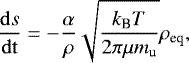
The sublimation prescription is taken from Lebreton et al. (2013, their Eqs. (17) and (18)), and follows the methodology described in Lamy (1974). The evolution of the grain size s reads
 (4)
(4)
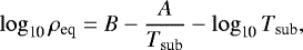
where ρ is the grain density, kB is the Boltzmann constant, T is the grain temperature, μ is the mean molecular mass of the considered dust composition, and mu is the atomic mass unit. The equilibrium gas density ρeq around the grain is given by
 (5)
(5)
with Tsub being the sublimation temperature of the grain. We have assumed that the pressure of the gas surrounding the grain (ρgas in Lebreton et al. 2013) is negligible, and the efficiency factor α to be 0.7, asin Lamy (1974). The thermodynamical properties are documented in Table 2 for each of the three compositions considered in this paper. The sublimation prescription used here is similar to that used by Kobayashi et al. (2011), with the transformations from one set of thermodynamical parameters to another given in Appendix B. At each timestep in the dynamical code, the mass lost by a grain due to sublimation is computed, and the grain size and the β value are modified accordingly for the next dynamical timestep. It is worth noting that the sublimation timescales can be very sensitive to the composition. In particular, the behavior of the glassy silicates is very different from that of the carbon and astrosilicate grains. For example, while it takes 2 × 10⁶ and 3 × 10⁶ s to entirely sublimate a carbon and an astrosilicate grain of 1 μm, respectively, once the sublimation temperature is reached, a glassy silicate grain of the same size will sublimate in only 102 s at its own sublimation temperature.
 |
Fig. 1 βpr for three different grain compositions around different spectral type stars (ticks correspond to the grain sizes used in our simulations). The solid horizontal line is the limit β = 0.5: grains over this value are blown out by radiation pressure if produced from circular orbits. The dashed horizontal line is the limit β = 1: grains above this value are always expelled, regardless of the way they are produced. |
Grain parameters used in the code.
2.4 Synthetic spectral energy distributions
By combining the different, single-size (single-β) grain runs, we can estimate a density profile, as parameterized by the vertical optical depth τ, assuming that the grains are produced at steady state from the parent belt. The usual method consists in recording the grains positions at regularly spaced time intervals, and pile up these different positions following a procedure similar to that used by Thébault et al. (2012) until the grain is removed from the system (ejection, sublimation, or fall onto the star). Here, we employ a different approach to compute τ, described in detail in Appendix C. It combines density profiles derived from the limited number of test grains for which the dynamics have been calculated accurately, and timescale estimates for a broader range of grain sizes, to produce 2D (r, s) density and optical depth maps. These maps are obtained assuming an initial differential size distribution proportional to s−3.5.
We also developed a Python implemented version of the GRaTeR radiative transfer code (Augereau et al. 1999) that allows us to calculate thermal emission and scattered light maps at any wavelength from the 2D (r, s) maps, as well as spectral energy distributions (SED) of the exozodis in order to directly compare our numerical results with the observations.
3 PR-drag pile-up scenario
We consider a setup similar to the one explored by Kobayashi et al. (2011) and Van Lieshout et al. (2014), with a population of small grains assumed to be released by collisions in a Kuiper belt-like ring (parent bodies located at r0 = 50 au), whose evolution is then followed, taking into account PR-drag and sublimation near the star, until the grains leave the system either by total sublimation, by falling onto the star, or by dynamical ejection. We explore four stellar types and three different grain compositions (see Tables 1 and 2). We consider 24 initial grain sizes, ranging from 1.7 nm to 1 mm, and thus 24 different initial β values (vertical tick marks in Figs. 1a, b, and c). We consider that the grains are released from parent bodies on circular orbits at r0 = 50 au, so that the grains’ initial orbit is given by a = r0 × (1 − β)∕(1 − 2β) and e = β∕(1 − β).
3.1 Grain evolution
3.1.1 General behavior
Figures 2 and 3 present the evolution of grain sizes and orbital elements for a subset of the explored parameter space (stellar type, grain composition).
As can be seen, the initial stage (labeled “stage I”, after Kobayashi et al. 2009, and reproduced in Figs. 2c and d) is similar for all cases and corresponds to the behavior found by previous studies using orbit-averaged equations: the grain drifts inward due to PR-drag, and its orbit is progressively circularized, while its size remains constant because it is too far from the sublimation region. We note, however, that contrary to the predictions of orbit-averaged prescriptions, the eccentricity stops decreasing at a given point and starts to slowly increase again as its semi-major axis continues to drop (named Stage Ib in Fig. 2d). This inflection point corresponds to a residual value below which the osculating eccentricity of the PR-drag drifting particle cannot fall, which is due to the intrinsic curvature of the tightly wound spirals that the grain actually follows as it migrates inward. The osculating eccentricity corresponding to these spirals can be approximated to a first order by (da/a)orb, which is the relative variation of the particle’s semi-major axis, due to PR-drag, over one orbital period as given by the averaged equations used by Kobayashi et al. (2009) or Van Lieshout et al. (2014). Taking the right-hand term of Eq. (1) in Kobayashi et al. (2011) (drift rate due to PR-drag), we get
 (6)
(6)
where T is the orbital period and c the speed of light. This leads to a residual eccentricity on the order of
 (7)
(7)
which increases with decreasing a. This non-zero eres is always relatively small, less than a few 10−3, but it cannot be ignored because even such a small value can make a difference in the fate of a grain as it starts sublimating.
As expected, the situation radically changes as the grains approach the sublimation region. As already identified in previous studies, as the grains start to sublimate, radiation-pressure increases and eventually halts their inward drift. During this “stage II” (again following Kobayashi et al. 2009), the grain shrinks while staying at its sublimation radius rs, which does not always correspond to a constant distance to the star because grain temperatures, and thus their sublimation distance, depend on their size (see, e.g., Fig. 2e). In parallel with this size decrease, the grain’s eccentricity increases rapidly. At one point, this eccentricity becomes significant enough for the particle to spend only a very small fraction of its orbit in the narrow sublimating region around rs. The grain then enters “stage III” where its sublimation drastically slows down, only occurring at periastron passages. Its orbital eccentricity continues to increase, albeit more slowly than before, receiving additional kicks at each sublimating-periastron passage.
The fate of the grain was not investigated in Kobayashi et al. (2009) or Van Lieshout et al. (2014) because it occurs in a fast-evolving regime where orbit-averaged equations are no longer valid. The fate depends on the dust composition and the stellar type. This is discussed in detail below.
3.1.2 Ejection
In most cases, the dust grain is parked on these ever-more-eccentric orbits, all having their periastron at rs, until its eccentricity reaches 1 and the grain is ejected from the system. By the time it reaches the e = 1 limit, its β is higher than the classical 0.5 value expected for a grain released from a β = 0 progenitor on a circular orbit (Fig. 4); when grains start to sublimate in stage II, PR-drag is still able to force their eccentricities to low values, lower than they should have according to the canonical e = β∕(1 − β) relation. So that once sublimation becomes really intensive and the grain approaches the β = 0.5 value, its eccentricity is still relatively small, allowing it to stay on a bound orbit beyond this critical 0.5 value. The highest possible β value for a grain reaching e = 1 is β = 1, obtained for an idealized case where the e = 1 grain is produced from a β = 0.5 progenitor on a circular orbit. However, in practice, we never obtain β values exceeding 0.8–0.85 (see Fig. 4 for the simulation leading to the highest beta values for e = 1 particles), which is because the grains’ eccentricities are never exactly zero as they enter stage II. And even values as small as a few 10−4 are enough to prevent the orbit from reaching β = 1 by the time it reaches e = 1. This can be understood by looking at Eq. (58) of Kobayashi et al. (2009) and Eq. (48) of Van Lieshout et al. (2014), which give the evolution of e during stage II as a function of the initial e when it enters this stage.
The fact that β < 0.85 by the time the grains are ejected has important consequences. It means that the DDE always remains negligible because its magnitude only becomes significant for β values very close to 1. Taking Eqs. (2) and (3), the ratio of the DDE force to the radiation pressure plus PR-drag force along the velocity reads
 (8)
(8)
For the highest β value obtained in our runs, i.e., 0.85 for an F0 star and carbon grains, we get a maximum FDDE∕FPR value of 0.03. We can thus safely conclude that DDE only has a very marginal influence on the grains’ evolution, whose effect can be neglected on the density pile-up of grains close to rs.
3.1.3 Total sublimation
For a small subset of our simulations, the grains’ fate is radically different, as they are removed from the system by total sublimation. These correspond to the specific cases of a G0 star and glassy silicates, and of a K0 star for both astrosilicate and glassy silicates (Fig. 3). The behavior for the K0 cases is easy to understand: the maximum possible β value is indeed always below 1, regardless of particle size (Fig. 1). This means that, as they sublimate during stage II, grains will never reach β values high enough for them to reach the e = 1 limit. They will thus stay on bound orbits all the time, while still sublimating at their orbital periastron, so that they eventually get fully sublimated. As a consequence, the grains that reach the maximum possible β value will survive longer than grains close in size, but with smaller β values.
For a G0 star and glassy silicates, β can exceed one, but only in a relatively narrow size range (see Fig. 1c). As a consequence, as it sublimates, the radius of a grain can directly cross the whole β > 1 size domain, and even sometimes the β > 0.5 domain, before having the time to be pushed on an unbound orbit. The fate of a grain is very difficult to predict in advance, as it strongly depends on its orbital location by the time it begins to significantly sublimate. All we can safely establish is that there is a significant fraction of grains that will disappear because of full sublimation (Fig. 3a).
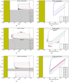 |
Fig. 2 PR-drag pile-up scenario: grain evolution as a function of initial grain size for three different stellar types and two grain compositions. Left panels: grain size as a function of stellar distance. The arrows denote the temporal evolution. The dash-dotted line is the sublimation distance as a function of grain size, while the vertical dashed line indicates the position of the parent bodies. The gray horizontal zone identifies the range of grains with β > 1, and the horizontal dotted lines correspond to β = 0.5 (see also Fig. 1). Right panels: eccentricity as a function of semi-major axis. The horizontal plain line represents the e = 1 limit beyond which particles are on unbound orbits. For both the left and right panels, the left yellow area corresponds to the physical location of the star and the arrows denote the evolution way. |
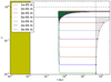 |
Fig. 4 PR-drag pile-up scenario: evolution of β as a function of stellar distance r for the initially bound astrosilicate grains around the A0 star. The parent belt is located at 50 au (vertical dashed line), and the grains are released on increasingly eccentric orbits as β raises. The arrows represent the inital apoastron of the grains. |
3.2 Global disk properties and spectra
3.2.1 Grain size
Figure 5 and Table 3 provide an overview of the smallest grain sizes that can be reached for our sample of stars and grain compositions. We see that for early-type stars we are unable to produce submicron-sized grains regardless of the considered grain composition. This absence of submicron-sized grains also extends to the case of late-type stars when considering carbonaceous dust. These results are in apparent contradiction with constraints on dominant grain sizes derived from precisespectral modeling of observed exozodis, which always tend to favor submicron-sized dust (see Sect. 1).
The only cases for which submicron-sized grains are produced are those where the grain can experience full sublimation, i.e., those for which the maximum possible β value is lower than 1 or barely exceeds it. As is discussed in Sect. 3.1.3, this is only true for K0 stars (astro- and glassy silicates) and G0 stars (glassy silicates only). However, even in these cases the lifetime of such tiny grains is very short (sublimation being very fast and efficient), which might not be enough to leave an observable signature.
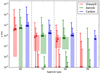 |
Fig. 5 Arrows representing the initial to final grain size evolution for a sample of simulations. The arrow head corresponds to the ejection size, or to total sublimation if it reaches the bottom of the figure. The colored rectangles are the range of grain sizes for which β > 0.5. |
PR-drag pile-up scenario: minimal distance and grain size reached for each configuration.
3.2.2 Surface density profiles
Another prediction of radiative transfer models of exozodis is that the hot dust is expected to be confined close to its sublimation radius. In order to evaluate the level of dust pile-up at rs, we compute the radial distribution of the total geometrical optical depth, τ, of the dust produced by the PR-drag scenario, following the approach described in Appendix C.
As can be seen in Fig. 6, the τ(r) profiles are almost flat for most of the domain between the release belt position down to rs, which is the expected result for a PR-drag scenario (Burns et al. 1979). The only departure from the flat profile occurs close to the sublimation radius, rs, where we obtain a dust pile-up generating a density enhancement of a factor of a few at most (earliest type stars, carbon grains) with respect to the plateau at larger distance, which is compatible with the values obtained by Van Lieshout et al. (2014). This enhancement is due to the biggest grains sublimating at rs, all passing through the (r,s) = (0.2 au, 10−5 m) bin in the 2D maps in the case of an A0 star and carbon grains (see also the upper left panel of Fig. 8) before being expelled. The radial extent of this pile-up is also very narrow, and is only marginally resolved in our simulations. Thus, we can constrain the enhancement to occur over less than 10−2 au, corresponding to a ratio Δr∕r of around 0.1. We note that for astrosilicates and glassy silicates the pile-up is even weaker than for carbon grains because for most stellar types, the β ratio is below 1 for the smallest grains of these compositions (Fig. 1). This means that as grains start to sublimate close to rs, they will not stay a long time on eccentric orbits (the reason for the pile-up) before sublimating completely.
3.2.3 SED
As mentioned in the introduction, the best way to evaluate how well our numerical scenario is able to explain exozodis observations is not to estimate how it reproduces the predictions of radiative transfer models regarding dust size or pile-up, but rather to evaluate how well it reproduces the observational constraints themselves. To this end, we use the Python version of the GRaTeR code developed for this study to generate synthetic SEDs. As explained in Sect. 2.1, because we neglect collisional effects in the parent belt, we cannot constrain the absolute level of dustiness, and thus the absolute near-IR fluxes, but we can focus on the relative balance between the near-IR and mid-IR fluxes as the main criteria to assess the validity of exozodi producing scenarios. As a consequence, we chose to rescale all our synthetic SEDs in order for the emission at 2 μm to correspond to the level measured for four observationally detected exozodis corresponding to the four different spectral types considered: Vega (A0), η Corvi (F0), 10 Tau (G0), and τ Ceti (a G8 star that is relatively close to a K0 star). For all these cases, we note that the flux excess at 2 μm is always on the order of ~1% of the stellar contribution.
The four corresponding synthetic SEDs are shown in Figs. 7a–d. We clearly see, for all considered spectral types and grain compositions, that the shape of the synthetic SED contradicts the observational constraints. The synthetic SEDs peak in the far-IR and the flux density in the 10–20 μm domain is always much higher than that found in exozodi observations, which are only a small percent of the stellar flux around 10 μm. This clearly illustrates the fact that the pile-up near the sublimation region is far from being sufficient to boost the near-IR flux at the point where it can dominate over the mid-IR flux. This mid-IR flux excess is due to the continuous flow of PR-drag drifting grains in the region between the production belt and rs. This can be clearly seen in Fig. 8, which shows, for the two extreme cases of A0 and K0, the contributions of the grains to the fluxes at 2 and 10 μm as a function of their size and spatial location.
We checked whether one way to alleviate this problem could be to start with a parent belt much closer than the considered 50 au. We reproduce this situation in a simple manner without running additional simulations. We consider our original simulations with a parent belt at 50 au, and integrate the flux coming from the grains within a given distance to the star. That distance is assumed to mimic the new location of the parent belt. In the specific case of Vega, the results are shown in Fig. 7e, where all fluxes have been normalized to the same observed flux at λ = 2.12 μm. The “unwanted” mid-IR (10 μm) flux falls to observation-compatible levels only for an extremely close-in parent belt located at 0.4 au. This solution appears highly unlikely given that such a massive collisional belt would probably not be able to survive longenough so close to the star to sustain the hot dust for a duration comparable to the age of the star.
Overall, these conclusions hint at a production process other than the PR-drag mechanism to populate the hot exozodiacal dust systems.
 |
Fig. 6 PR-drag pile-up scenario: radial profiles for the size-integrated geometrical optical depth for all grain compositions and stellar types. |
4 Exocometary dust delivery scenario
Another classic process of exozodiacal dust production is the cometary grain release very close to the star. In this scenario, an outer mass reservoir remains necessary, but the dust grains are deposited by large, undetectable parent bodies in the immediate vicinity of the place where they are detected. A benefit of this process compared to the PR-drag pile-up scenario is that it leaves essentially no observable signature between the parent belt and the exozodi.
In Bonsor et al. (2012), we investigated the planetary system architecture required to sustain an inward flux of exocomets. In Bonsor et al. (2014), we highlighted the importance of planetesimal-driven migration of the planet closest to the inner edge of the belt to maintain this flux on sufficiently long timescales (see also Raymond & Bonsor 2014). In Marboeuf et al. (2016), we evaluated the cometary dust ejection rate as a function of the distance to the star and spectraltype to help connect dynamical simulations to exozodi observations in future studies (e.g., Faramaz et al. 2017). Here, we take an important further step by discussing the fate of the grains once released by an exocomet passing close to the star, and by calculating the resulting emission spectra for a direct comparison to the data.
4.1 Numerical setup
In order to compare the outcome of our cometary model to the results obtained for the PR-drag pile-up scenario (Sect. 3), we consider a reservoir of exocomets whose aphelion is at a fixed distance of 50 au and whose perihelion rp is just outside the sublimation limit, which for each composition and spectral type we define as the largest sublimation distance of the considered grain sizes (often corresponding to the smallest grains; see vertical dashed lines in Figs. 9a–d).
We assume that all grains leaving the comet are produced when the comet passes at perihelion rp. This is a simplifying assumption because grains should be dragged from the comet by the evaporation of volatiles, which should happen overa large fraction of its orbit. However, as shown by Marboeuf et al. (2016), the volatile and dust production rate strongly increase with decreasing distance to the star (see Eq. (17) in that paper), so that most of the mass loss happens in a narrow region close to the comet’s perihelion, as is clearly illustrated in Fig. 10.
Grains produced at perihelion have the highest possible speed once released from the comet and are thus less likely to remain bound. More precisely, the blowout limit in term of β is lowered compared to the PR-drag pile-up scenario and can be expressed as (e.g., Murray & Dermott 1999)
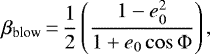 (9)
(9)
where Φ is the longitude of the release position on the cometary orbit and e0 the parent body eccentricity. This reduces to βblow = (1 − e0)∕2 for a release at perihelion. For the grain compositions and spectral types explored in this study (Sect. 2.3), the release distance varies between 2 and ~0.02 au, corresponding, for an apoastron of 50 au, to parent body eccentricities varying between 0.923 and 0.999, and βblow values between 3.8 × 10⁻² and 5.0 × 10⁻⁴, respectively. These low βblow values translate into large grain sizes, of several tens to several hundred of μm, for the limiting blowout size. The release distances, orbit eccentricities, blowout β values, and grain sizes sblow are documented in Table 4 for the four spectral types and three compositions investigated in this study.
4.2 Grain evolution
4.2.1 Carbon and astrosilicate grains
In our model, the carbon and astrosilicate bound grains (β < βblow, i.e., s > sblow) are delivered by an exocomet a little beyond their sublimation distance, leaving room for dynamical evolution. The fate of these grains shows similarities to that discussed in the case of the PR-drag pile-up scenario. Their semi-major axis and eccentricity both decrease by PR-drag, until they are totally sublimated (Sect. 3.1.3) or expelled from the system by radiation pressure due to partial sublimation (Sect. 3.1.2), as illustrated in Figs. 9c and d.
There are, however, important differences between the cometary and PR-drag pile-up scenarios. In particular, the high orbital eccentricity of the grains inherited from the comet implies that those grains spend only a very small fraction of their orbital period (typically less than a day) close to the sublimation zone in the early phases of their evolution. Therefore, these grains see their size remaining essentially constant while migrating inward by PR-drag, as in stage I of the PR-drag pile-up scenario (Sect. 3.1.1). Their orbit is getting circularized until sublimation becomes significant, thereby moving into the stage II phase. However, they enter this phase with a significant residual eccentricity (on the order of 0.1; see Fig. 9e), much larger than in the case of the PR-drag pile-up scenario. As a consequence, the carbon and astrosilicate grains are expelled when they reach a β value of about 0.6 (Fig. 9f), to be compared to the 0.8 accessible in the PR-drag scenario. The only exception is for astrosilicate grains around the K0-type star, for which the β = 0.6 value is never reached across all grain sizes, meaning that the bound grains end up completely sublimated. Another consequenceof the significant residual eccentricity during stage II is that here the grains again do not reach β values close enough to 1 for the DDE mechanism to operate.
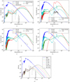 |
Fig. 7 Panels a–d: SED for each spectral type and all compositions in the PR-drag pile-up scenario. All spectra are normalized to the flux ratio at 2 μm, and compared to observed fluxes for exozodis around stars of similar type (for the F0 star, for which there is no available observed photometry at 2 μm, the valueis put to 1% of the stellar flux). Data points for Vega are from Absil et al. (2006), η Crv are from Lebreton et al. (2016), 10 Tau are from Kirchschlager et al. (2017), τ Cet are from Di Folco et al. (2007). Additional values are from Absil et al. (2013) and Mennesson et al. (2014). Panel e: SEDs for an A0 star and carbon grains, but only considering the flux within a radial distance indicated in the top right corner, and flux-normalized at λ = 2.12μm such that the disk flux amounts to 1.29% of the stellar flux at that wavelength (FLUOR excess for Vega). |
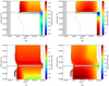 |
Fig. 8 PR-drag pile-up scenario: flux level at 2 μm (left) and 10 μm (right) for an A0 star and carbon grains (top); and K0 star and astrosilicate grains (bottom). See Sect. 2.4 and Appendix C for the methodology. The vertical dashed line corresponds to the location of the sublimation radius rs as a function of grain size, while the full and dashed horizontal lines indicate the β = 0.5 and β = 1 limits, respectively. |
4.2.2 Glassy silicate grains
The behavior of glassy silicate grains is quite different. The sublimation timescale of these grains at the sublimation temperature is four orders of magnitude lower than for the other compositions considered here (Sect. 2.3). In this case, the sublimation time becomes comparable to the time spent by the grain close to the sublimation limit in only one perihelion flyby. For the A- and F-type stars, this results in a complete sublimation of the bound grains after the circularization of stage II.
For later type stars, the fate of the bound grains is affected by the unusual fact that, at a given distance, large glassy silicate grains are hotter than smaller ones (see the almost vertical dash-dotted lines in Figs. 3 and 9b). Therefore, the large bound glassy silicate grains are released at, or very close to, their sublimation distance around late-type stars in our model. Their high temperature, combined with the intrinsic sublimation efficiency of glassy silicates compared to carbon and astrosilicate grains, implies that their sublimation timescale is in this case lower than the PR-drag timescale. As a consequence, these bound grains become small enough to be expelled before their orbits can be circularized.
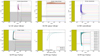 |
Fig. 9 Panels a–c: grain size as function of the distance for all simulations run in the exocometary dust delivery at perihelion scenario (the yellow area, and the dotted and dash-dotted lines have the same meaning as in Fig. 2, while the dashed line corresponds to the limit between initially bound and unbound grains sizes). Panels d–f: specific case of an F0 star and carbon grains, for which the evolution of the grain size, the eccentricity, and the β value as a function of distance is displayed. In the case of eccentricity, the two curves overlap. |
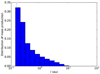 |
Fig. 10 Fraction of the surface mass loss for an exocomet orbiting an F0 star as a function of radial distance. The comet has an apoastron of 50 au, and an eccentricity of 0.994. Based on the comet evaporation prescription of Marboeuf et al. (2016, their Eq. (17)). |
4.3 Global disk properties and spectra
4.3.1 Surface density profiles
We calculate the radial distribution of the total geometrical optical depth, τ, of the dust produced in the comet-release scenario, following the approach described in Appendix C, and already used in the case of the PR-drag pile-up scenario (see Sect. 3.2.2). As illustrated in Fig. 11 for carbon grains, for a release at a perihelion rp that is close to the sublimation distance rs, the radial density profile peaks at the release location and decreases further out with the distance to the star as r−1.7.
To check the importance of the position of the periastron with respect to the sublimation distance, we performed an additional simulation, for an F0 star and carbon grains, for which the dust is released at 1 au insteadof 0.13 au in the nominal case. As can be seen in Fig. 11, we obtain a flat τ(r) profile in between rs and 1 au, followed by a r−1.7 profile at larger distances. The plateau between rp to rs results from the inward migration and circularization of the orbit of the bound grains by PR-drag, as already observed for the PR-drag pile-up scenario (Fig. 6), while the high-eccentricity bound grains populate the regions outside that distance. We conclude that the exocometary dust delivery position can essentially be regarded as playing the same role as the parent belt distance in the PR-drag pile-up scenario, as far as the shape of the τ(r) profile between that reference position down to the sublimation distance is concerned. Numerically, the PR-drag pile-up scenario can be considered an extreme case of the cometary scenario, with exocomets having zero eccentricity.
4.3.2 SED
We use the same computing and normalization approach as in Sect. 3.2.3 to evaluate the SEDs resulting from the exocometary dust production scenario. A notable difference with the PR-drag pile-up scenario is that it is possible here to connect the absoluteexozodiacal dust level to a number of exocomets passing close to the star (see Sect. 4.4 for further details).
The synthetic SEDs for the exocometary scenario are displayed in Fig. 12 for the four spectral types and three dust compositions considered in this study, and are compared to the same reference observed systems as in Fig. 7. Overall, the mid- to far-infrared excess is significantly reduced compared to the PR-drag pile-up scenario. This is mainly because the grains are directly deposited next to the sublimation zone, mitigating the amount of dust beyond the grain release position (the comet’sperihelion). The peak of the SED is accordingly shifted to much shorter wavelengths compared to the PR-drag pile-up scenario.
In this respect, the carbon grain case is the most favorable one. Regardless of the spectral type, the exozodiacal emission of cometary carbon grains peaksat 3–5 μm. The flux at 10 μm is always significantly smaller than the stellar flux at the same wavelength, by a factor of about five, even though it is still not enough to fully fit the data. The models with astrosilicate and glassy silicate grains, on the other hand, predict emissions that are much too large in the mid- and far-infrared compared to the observations of hot exozodis.
In Fig. 12b we also display the SED obtained for the case with a comet perihelion at rp = 1 au, far away from the sublimation distance rs. As can be clearly seen, the fit to the observed data is much poorer because of the excess mid-IR flux due to PR-drag drifting grains in the flat region between rp and rs that was identified in Fig. 11. In essence, here we are close to the cases explored in the PR-drag pile-up scenario (Sect. 3).
The main contributors to the flux at different wavelengths can be explored using 2D emission maps as a function of the grain size and distance to the star. Figure 13a–d show examples for our best case, i.e., an F0 star and a carbon dust composition. We see that the near- and mid-IR emissions essentially come from the same relatively large grains (several tens to hundreds of micrometers), which are the smallest bound grains released by the exocomets (Table 4). At 2 μm, most of the flux originates from the smallest bound grains just outside the sublimation distance, while the 10 μm emission comes from grains similar in size but distributed over a broader region centered around the dust release position (Fig. 13b). At that wavelength, the drop in the surface density beyond the dust delivery position (0.13 au) contributes to moderating the emission from the distant regions, as was demonstrated in the PR-drag pile-up scenario when we schematically simulated much closer-in parent belts (Fig. 7). These behaviors at 2 and 10 μm are emphasized when the exocomet’s perihelion is arbitrarily moved to 1 au, as shown in Fig.13c and d. Finally, we note that a direct consequence of the fact that the emission originates from large grains is that the strong silicate features seen in the case of the PR-drag pile-up scenario are essentially absent here.
Overall, it is noteworthy that two key features of the classical radiative transfer models of exozodis (e.g., Absil et al. 2006, and following studies) are reproduced with the exocometary dust delivery scenario, namely an accumulation of the grains very close to the sublimation zone and a preference for carbon-rich dust. Nevertheless, it should also be noted that the carriers of the exozodi emission in that case are several orders of magnitude larger in size than the grains usually required by the classical radiative transfer models.
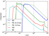 |
Fig. 11 Total geometrical optical depth (τ) in the exocometary dust delivery at perihelion scenario, assuming carbon grains. For illustrative purposes, a model with an exocomet perihelion larger than in the nominal case is shown for the F0 star. |
Parameters for the cometary release at perihelion scenario.
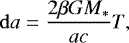
4.4 Inward flux and size of the exocomets
As already mentioned in the previous sections the flux was arbitrarily rescaled in order to match the observed excess levels in the near-IR. Now, in order to discuss further the relevance of the exocometary dust delivery scenario, we aim to evaluate the size and number of exocomets required to physically reach these observed exozodiacal flux level. For this purpose, we employ the cometary dust ejection prescription of Marboeuf et al. (2016), in particular their Eq. (17), together with the orbital parameters documented in Table 4, to quantify the mass of grains released by a comet over an orbital period. This also allows us to estimate, for a given comet mass, the exocomet lifetime as well as the number of orbits before complete erosion. These quantities are used to assess the absolute flux density at 2 and 10 μm resulting from the evaporation of an exocomet of a certain size. The different steps of the adopted methodology are detailed in Appendix D, and the results for a typical 10 km exocomet are summarized in Tables D.1 and D.2.
In the case of carbon and astrosilicate grains, the flux produced at 2 μm by one 10 km exocomet amounts to a few 10−5 to a few 10−4 the stellar flux at the same wavelength. Therefore, a few tens to a few hundreds of active 10 km radius exocomets on a similar orbit are required to reach the observed level of ~1% of the stellar flux at 2 μm. At 10 μm, the dust-to-star flux ratio is always larger than at 2 μm, by a factor of about 20 for the carbon grains, and a factor of about 200 for the astrosilicate grains, in agreement with the results in Sect. 4.3.2. The required number of active exocomets can be mitigated if their initial size is larger. Because we consider the total flux resulting from the complete erosion of the exocomet, it scales directly with the exocomet mass and hence with the exocomet radius to the cube. Therefore, a single active 40–80 km exocomet would be enough to produce a 1% excess at 2 μm. Glassy silicate fluxes are significantly lower due to the short sublimation lifetime of such grains. Around FGK stars, these grains sublimate significantly at each perihelion passage, and disapear in a few orbits.
Several assumptions enter into the calculation of the number and size of the exocomets required to reproduce the observations (see Sect. 4.1 and Appendix D), and the above values should therefore be taken with caution. It should also be remembered that our conclusions are valid for the specific orbital parameters summarized in Table 4. Nevertheless, the results are encouraging in the sense that the sizes and number of exocomets appear reasonable, thereby providing additional support to the exocometary dust delivery scenario explored in this study.
5 Summary and conclusion
By investigating, via non-orbit-averaged equations, the fate of dust around several different stellar types, and considering different grain compositions, we are able to draw some conclusions on the properties of exozodis emission depending whether these grains come from an outer parent belt and drift inward by PR-drag (Sect. 3) or if they have an exocometary origin (Sect. 4). We show the following:
-
In the case of the PR-drag pile-up scenario:
-
for early-type stars, significant amounts of submicrometer-sized grains cannot be produced in the inner disk regions because grains are blown out by radiation pressure before sublimating down to these sizes. The only case for which submicrometer-sized grains are obtained is that of silicate grains around late-type stars;
-
dust pile-up close to the sublimation radius is moderate, generating a density enhancement of a few at most with respect to an otherwise flat surface density profile;
-
the near-IR excess is always associated with mid-IR excess at the same level, or even much higher. This behavior cannot explain the numerous near-IR excesses without mid-IR excess detections.
-
-
In the case of the exocometary dust delivery scenario:
-
a narrow ring forms close to the sublimation zone near the comet’s periastron. This ring is predominantly populated with large grains, a few tens to a few hundred μm in radius depending on the composition, which are the smallest bound grains produced at the comet’s perihelion;
-
compared to the PR-drag pile-up scenario, the near-IR excess is associated with a much smaller mid-IR excess, in better agreement with the data, although not totally fitting them. Carbon-rich grains provide the best results;
-
the near-IR excess can be reproduced assuming realistic inward fluxes of exocomets and reasonable exocomet sizes.
-
In addition, we find that the DDE mechanism, which could in principle help form a dense dust ring close to the sublimation radius, has a very limited effect in both scenarios because particles never reach β values close enough to 1 by the time they are blown out.
Therefore, based on simulations performed with the new numerical model developed in the context of this study, we conclude that the PR-drag pile-up scenario is unlikely to produce the hot exozodis observed with near-IR interferometry. The exocomet release at perihelion scenario, on the other hand, provides a very promising theoretical framework that should be explored further. To this end, future developments of our numerical model will include a post-processing treatment of the collisions in the dust ring close to the sublimation zone, building up on the DyCoSS collisional model used in the context of debris disks (e.g., Thébault et al. 2012, 2014). It should also include a detailed calculation of the grain charging, following for instance the prescription of Kimura et al. (2019), and a careful consideration of the magnetic topology in order to thoroughly discuss the efficiency of magnetic trapping and its impact on the near- and mid-IR emissions.
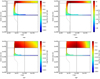 |
Fig. 13 Contribution of each size and distance bin to the flux at 2 μm (left) and 10 μm (right) in the case of an F0 star and carbon grains. The grains are released by a exocomet at 0.13 au (top) and 1 au (bottom). |
Acknowledgements
We thank Hiroshi Kimura for providing the optical constants for glassy silicates, and for the discussions about the DDE mechanism. We also thank Rik van Lieshout for the useful discussion concerning sublimation processes. We acknowledgethe financial support from the Programme National de Planétologie (PNP) of CNRS-INSU co-funded by the CNES. Our code uses the NumPy (Oliphant 2006) and the Matplotlib libraries (Hunter 2007). This work has made use of data from the European Space Agency (ESA) mission Gaia (https://www.cosmos.esa.int/gaia), processed by the Gaia Data Processing and Analysis Consortium (DPAC, https://www.cosmos.esa.int/web/gaia/dpac/consortium). Funding for the DPAC has been provided by national institutions, in particular the institutions participating in the Gaia Multilateral Agreement.
Appendix A Reproducing Krivov et al. (1998)
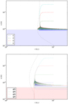 |
Fig. A.1 Top: evolution of the grain size as a function of the distance to the Sun for carbon grains of initial sizes 1, 3, 10, and 30 μm. Bottom: same, but for the glassy silicate. These plots reproduce the results presented in Fig. 5 of Krivov et al. (1998). |
Appendix B Thermodynamical properties
The literature is rich in two-parameter formulae for describing the sublimation process of dust grains, which are in essence similar, but with different notations, which creates some confusion. Here we propose a summary of the equations to transform the two parameters in four different papers in the literature to the (A, B) parameters of Lebreton et al. (2013) used in this study:
-
(AZ, MZ) parameters in Zavitsanos & Carlson (1973), table 3:

The value of 6 in the expression for B, coming from the unit system, is not present in Lebreton et al. (2013), which explains the difference in our derived values.
-
(H, P) parameters in Kobayashi et al. (2009):

-
(AC, BC) parameters in Cameron & Fegley (1982):

-
(A, BL) parameters in Lamy (1974):
 (B.7)
(B.7)
Appendix C Geometrical optical depth map computation
Our goal was to produce density and optical depth maps from trajectories independently computed for individual grains with our dynamical code (which includes sublimation). In the first step, we defined a 2D grid of logarithmically spaced distances to the star (r) and grain sizes (s). Then, for each single-grain size simulation, we summed up the times spent by the grain during its lifetime in each bin of the 2D grid, correcting this time by the initial differential size distribution assumed to be proportional to s−3.5 (collisional erosion). This yielded a first 2D map of cumulative times, which is proportional to a density map if the system is assumed to be at steady state. As illustrated in Fig. C.1, the limited number of grain sizes for which the dynamics were computed leaves empty grain size bins in the 2D map (empty lines). This led us to develop a complementary approach to fill the holes in this map.
We defined a second 2D (r,s) map of the same size and same bin values as the first 2D map. We then estimated three timescales for each bin in the 2D (r,s) map to qualitatively evaluate the ability of a grain to move to a nearby bin due to sublimation, ejection (radiation pressure), or inward migration (PR-drag). The sublimation timescale to move from (ri, si) to (ri, si−1) and the ejection timescale to move from (ri, si) to (ri+1,si) are both taken from Lebreton et al. (2013). The PR-drag timescale to move from (ri, si) to (ri−1,si) is taken from Burns et al. (1979). In each bin, the shortest timescale gives the dominant physical process and this is used to predict the trajectory of a grain in the 2D map, allowing a jump from position (ri, si) to (ri−1,si−1) when sublimation and PR-drag migration timescales are comparable. This is illustrated in Fig. C.2, where we can see that sublimation is the dominant physical process close to the sublimation distance for the smallest grains, while inward migration is the dominant physical process for the biggest grains, and ejection dominates over the other processes otherwise.
This second 2D map provides crude evolution tracks for the grains that are used to populate another cumulative time map similar to the one shown in Fig. C.1. We proceeded as follows. For each size bin, we populate the initial position bin given the value of β, thereby accounting for the eccentricity of the orbit while the apoastron is fixed by the parent belt position. Then, we follow each synthetic grain along the (r, s) plane, with a path determined by the smallest timescale in each of the successive bins through which the grain is passing. Each local, smallest timescale is stored after being multiplied by the initial dust differential size distribution proportional to s−3.5, and summed up to give a complete map of cumulative times, covering all grain sizes. This is shown in Fig. C.3 and can be directly compared to the map obtained with the dynamical code (Fig. C.1).
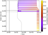 |
Fig. C.1 Cumulative time map derived from the simulations for the A0, carbon case. |
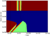 |
Fig. C.2 Dominant physical processes driving the evolution of a grain as a function of the distance to the star and grain size. Shown are inward migration by PR-drag (red), sublimation (green), a combination of both (orange), and ejection by radiationpressure (blue) (see text for more details on how the dominant process is estimated). |
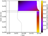 |
Fig. C.3 Cumulative time map derived from the estimated timescales for the A0, carbon case. |
We see that the 2D (r,s) map obtained with the dynamical code better follows the impact of changing β values due to sublimation; specifically, it better captures the dynamics of the grains just above the blowout size. These grains produce the so-called (and well-documented) pile-up close to the sublimation distance, which is not recovered in the 2D map built using typical timescales. The two cumulative time maps are then combined to produce a single, smooth map, where averaged values are taken when the bins are non-zero in both maps. This combined map can be regarded as a density map.
To get an optical depth map, the density map is multiplied by the geometrical cross-section in each bin, and divided by the distance to the star. This optical depth is thus vertically and azimuthally integrated. This can be used to construct the optical depth radialprofile by integrating over all grain sizes for example, or as a pre-requisite to evaluate the flux in scattered light and thermal emission (see Fig. 8). The 2D maps can also be used to truncate the disk, to estimate the emission within a certain radius for example.
For the sake of comparison, throughout the paper the maps shown are normalized to get a dust disk-to-star flux ratio of 1% at λ = 2 μm.
Appendix D Flux level produced by an evaporating exocomet
Here, we describe the methodology employed to compute the amount of dust released by the exocomets and the resulting flux density. Thesteps are the following:
- 1.
For each set of exocometary orbital parameters (see Sect. 4.1 and Table 4), we calculate the total mass of dust per unit of exocomet surface (in kg m−2) released by the exocomet in one complete revolution. This is done by integrating Eq. (17) of Marboeuf et al. (2016) along the exocomet orbit over one orbital period. The exocomet is thought to be composed of 50% dust. The results are independent of the actual size of the exocomet, but depend on the assumed grain size distribution. In the model of Marboeuf et al. (2016), the mass is calculated assuming a differential grain size distribution proportional to s−3.5 between smin = 1 μm and smax = 1 mm.
- 2.
An exocomet radius is assumed to get the exocomet surface and hence the total mass of dust ejected from the exocomet in one orbit using the result of the previous step. The released dust masses are documented in the row 6 of Tables D.1 and D.2, assuming an initial exocomet radius of 10 km.
- 3.
We make the approximation that all the dust ejected by the exocomet during one orbit is released at perihelion. Although this may appear a crude approximation, Fig. 10 shows that it is reasonable because a large fraction of the mass is produced close to the star, due to the high eccentricities considered in our study, and because the mass loss rate decreases as the distance squared to the star in the innermost regions (inside the water ice sublimation distance in the model of Marboeuf et al. 2016, see their Eq. (17)).
- 4.
This mass is distributed over the grain size bins of our model grid (see Appendix C) between 1 mm down tothe smallest grain size in our simulation, assuming a differential grain size distribution proportional to s−3.5. This step allows each size bin to be populated with an absolute number of grains. We note that the smallest size of our grid is lower than the smin = 1 μm lower limit adopted by Marboeuf et al. (2016), but the fraction of the total mass contained in the smallest grains is negligible with the adopted size distribution. Moreover, only the bound grains are kept in the next steps;
- 5.
This setup is used to produce a 2D map of cumulative times, as described in Appendix C, weighted by the absolute number of grains of each size obtained at the previous step. The 2D map is obtained by evolving the grains in position and size over the largest lifetime of the biggest grains (row 3 of Tables D.1 and D.2) (see Appendix C for the methodology). This step assumes in essence a system at steady state and is equivalent to populating the orbits to produce a density map. The 2D map is normalized by the time over which the simulation was evolved (row 3 of Tables D.1and D.2) to obtain a mean 2D number density map equivalent to a density map assuming a constant dust production process at perihelion. This procedure is valid if the grains released at the comet’s perihelion that dominate the flux survive long enough for their positions to be randomized in longitude along their orbits. We have checked that, in the case of the A0 star and carbon grains, the orbital periods vary by a factor of five within the considered grain range. This guaranties randomization in longitude within a few orbits, i.e., ~1000 yr in this case, to be compared with the grain lifetime which is typically two orders of magnitude larger;
- 6.
The mean 2D number density map is used to directly compute the absolute scattered light and thermal emission at the wavelength of 2 μm, providing an estimate of the mean flux density resulting from the first passage of a exocomet (row 7 in Tables D.1 and D.2). As time goes on, the exocomet radius shrinks. The number of exocomet orbits before complete sublimation and the exocomet lifetimes are documented in the rows 4 and 5 of Tables D.1 and D.2, respectively. The total flux density at 2 μm, produced by all the grains released by the exocomet over its lifetime, is then obtained by summing up the contributions at each successive perihelion passage until complete erosion of the exocomet (row 8 of Tables D.1 and D.2). The flux at 10 μm (row 9 of Tables D.1 and D.2) is computed in a similar way.
Parameters and flux for the A0 and F0 stars, resulting from the exocomet evaporation model, assuming a 10 km exocomet.
References
- Absil, O., di Folco, E., Mérand, A., et al. 2006, A&A, 452, 237 [NASA ADS] [CrossRef] [EDP Sciences] [Google Scholar]
- Absil, O., di Folco, E., Mérand, A., et al. 2008, A&A, 487, 14 [Google Scholar]
- Absil, O., Kervella, P., Mollier, B., et al. 2013, A&A, 555, A104 [NASA ADS] [CrossRef] [EDP Sciences] [Google Scholar]
- Akeson, R. L., Ciardi, D. R., Millan-Gabet, R., et al. 2009, ApJ, 691, 1896 [NASA ADS] [CrossRef] [Google Scholar]
- Augereau, J.-C., Lagrange, A.-M., Mouillet, D., Papaloizou, J. C. B., & Grorod, P. A. 1999, A&A, 348, 557 [Google Scholar]
- Belton, M. J. S. 1966, Science, 151, 35 [NASA ADS] [CrossRef] [Google Scholar]
- Beust, H., & Morbidelli, A. 2000, Icarus, 143, 170 [NASA ADS] [CrossRef] [Google Scholar]
- Bonsor, A., Augereau, J.-C., & Thébault, P. 2012, A&A, 548, A104 [NASA ADS] [CrossRef] [EDP Sciences] [Google Scholar]
- Bonsor, A., Raymond, S. N., & Augereau, J.-C. 2013, MNRAS, 433, 2938 [NASA ADS] [CrossRef] [Google Scholar]
- Bonsor, A., Raymond, S. N., Augereau, J.-C., & Ormel, C. W. 2014, MNRAS, 441, 2380 [NASA ADS] [CrossRef] [Google Scholar]
- Burns, J. A., Lamy, P. L., & Soter, S. 1979, Icarus, 40, 1 [NASA ADS] [CrossRef] [Google Scholar]
- Cameron, A. G. W., & Fegley, M. B. 1982, Icarus, 52, 1 [NASA ADS] [CrossRef] [Google Scholar]
- Czechowski, A., & Mann, I. 2012, Astrophys. Space Sci. Lib., 385, 47 [NASA ADS] [CrossRef] [Google Scholar]
- Defrère, D., Absil, O., Augereau, J.-C., et al. 2011, A&A, 534, A5 [NASA ADS] [CrossRef] [EDP Sciences] [Google Scholar]
- Dermott, S. F., Jayaraman, S., Xu, Y. L., Grogan, K., & Gustafson, B. A. S. 1996, Am. Inst. Phys. Conf. Ser., 348, 25 [NASA ADS] [Google Scholar]
- Di Folco, E., Absil, O., Augereau, J.-C., et al. 2007, A&A, 475, 243 [NASA ADS] [CrossRef] [EDP Sciences] [Google Scholar]
- Draine, B. T. 2003, ApJ, 598, 1026 [NASA ADS] [CrossRef] [Google Scholar]
- Ducati, J. R. 2002, VizieR Online Data Catalog: II/237 [Google Scholar]
- Ertel, S., Absil, O., Defrère, D., et al. 2014, A&A, 570, A128 [NASA ADS] [CrossRef] [EDP Sciences] [Google Scholar]
- Ertel, S., Defrère, D., Absil, O., et al. 2016, A&A, 595, A44 [NASA ADS] [CrossRef] [EDP Sciences] [Google Scholar]
- Ertel, S., Defrère, D., Hinz, P. M., et al. 2018, AJ, 155, 194 [NASA ADS] [CrossRef] [Google Scholar]
- Faramaz, V., Ertel, S., Booth, M., Cuadra, J., & Simmonds, C. 2017, MNRAS, 465, 2352 [NASA ADS] [CrossRef] [Google Scholar]
- Gaia Collaboration (Prusti, T., et al.) 2016, A&A, 595, A1 [NASA ADS] [CrossRef] [EDP Sciences] [Google Scholar]
- Gaia Collaboration (Brown, A. G. A., et al.) 2018, A&A, 616, A1 [NASA ADS] [CrossRef] [EDP Sciences] [Google Scholar]
- Hunter, J. D. 2007, Comput. Sci. Eng., 9, 90 [NASA ADS] [CrossRef] [Google Scholar]
- Kama, M., Min, M., & Dominik, C. 2009, A&A, 506, 1199 [NASA ADS] [CrossRef] [EDP Sciences] [Google Scholar]
- Kiefer, F., Lecavelier des Etangs, A., Augereau, J.-C., et al. 2014a, A&A, 561, L10 [NASA ADS] [CrossRef] [EDP Sciences] [Google Scholar]
- Kiefer, F., Lecavelier des Etangs, A., Boissier, J., et al. 2014b, Nature, 514, 462 [NASA ADS] [CrossRef] [EDP Sciences] [Google Scholar]
- Kiefer, F., Lecavelier des Etangs, A., Vidal-Madjar, A., et al. 2017, A&A, 308, A132 [NASA ADS] [CrossRef] [EDP Sciences] [Google Scholar]
- Kimura, H., Ishimoto, H., & Mukai, T. 1997, A&A, 326, 263 [NASA ADS] [Google Scholar]
- Kimura, H., Kunitomo, M., Suzuki, T. K., et al. 2019, Planet. Space Sci., in press DOI: 10.1016/j.pss.2018.07.010 [Google Scholar]
- Kirchschlager, F., Wolf, S., Krivov, A. V., Mutschke, H., & Brunngräber, R. 2017, MNRAS, 467, 1614 [NASA ADS] [Google Scholar]
- Kobayashi, H., Watanabe, S.-i., Kimura, H., & Yamamoto, T. 2008, Icarus, 195, 871 [NASA ADS] [CrossRef] [Google Scholar]
- Kobayashi, H., Watanabe, S.-i., Kimura, H., & Yamamoto, T. 2009, Icarus, 201, 395 [NASA ADS] [CrossRef] [Google Scholar]
- Kobayashi, H., Kimura, H., Watanabe, S.-i., Yamamoto, T., & Müller, S. 2011, Earth Planet Space, 63, 1067 [NASA ADS] [CrossRef] [Google Scholar]
- Kral, Q., Krivov, A. V., Defrère, D., et al. 2017, Astron. Rev., 2857, 1 [Google Scholar]
- Krivov, A. V. 2010, Res. Astron. Astrophys., 10, 383 [NASA ADS] [CrossRef] [Google Scholar]
- Krivov, A. V., Kimura, H., & Mann, I. 1998, Icarus, 134, 311 [NASA ADS] [CrossRef] [Google Scholar]
- Lamy, P. L. 1974, A&A, 35, 197 [NASA ADS] [Google Scholar]
- Lamy, P. L. 1978, Icarus, 34, 68 [NASA ADS] [CrossRef] [Google Scholar]
- Lebreton, J., van Lieshout, R., Augereau, J.-C., et al. 2013, A&A, 555, A146 [NASA ADS] [CrossRef] [EDP Sciences] [Google Scholar]
- Lebreton, J., Beichman, C. A., Bryden, G., et al. 2016, ApJ, 817, 165 [NASA ADS] [CrossRef] [Google Scholar]
- Liou, J. C., Dermott, S. F., & Xu, Y. L. 1995, Planet. Space Sci., 43, 717 [NASA ADS] [CrossRef] [Google Scholar]
- Marboeuf, U., Bonsor, A., & Augereau, J.-C. 2016, Planet. Space Sci., 133, 47 [NASA ADS] [CrossRef] [Google Scholar]
- Mennesson, B., Absil, O., Lebreton, J., et al. 2013, ApJ, 763, 119 [NASA ADS] [CrossRef] [Google Scholar]
- Mennesson, B., Millan-Gabet, R., Serabyn, E., et al. 2014, ApJ, 797, 119 [NASA ADS] [CrossRef] [Google Scholar]
- Montesinos, B., Eiroa, C., Krivov, A. V., et al. 2016, A&A, 593, A51 [NASA ADS] [CrossRef] [EDP Sciences] [Google Scholar]
- Mukai, T., & Yamamoto, T. 1979, PASJ, 31, 585 [NASA ADS] [Google Scholar]
- Mukai, T., Yamamoto, T., Hasegawa, H., Fujiwara, A., & Koike, C. 1974, PASJ, 26, 445 [NASA ADS] [Google Scholar]
- Murray, C. D., & Dermott, S. F. 1999, Solar System Dynamics (Cambridge: Cambridge University Press) [Google Scholar]
- Nesvorný, D., Jenniskens, P., Levison, H. F., et al. 2010, ApJ, 713, 816 [NASA ADS] [CrossRef] [Google Scholar]
- Nuñez, P. D., Scott, N. J., Mennesson, B., et al. 2017, A&A, 113, 1 [Google Scholar]
- Oliphant, T. E. 2006, A guide to NumPy (USA: Trelgol Publishing) [Google Scholar]
- Pollack, J. B., Toon, O. B., & Khare, B. N. 1973, Icarus, 19, 372 [NASA ADS] [CrossRef] [Google Scholar]
- Rappaport, S., Vanderburg, A., Jacobs, T., et al. 2018, MNRAS, 474, 1453 [NASA ADS] [CrossRef] [Google Scholar]
- Raymond, S. N., & Bonsor, A. 2014, MNRAS, 442, 18 [NASA ADS] [CrossRef] [Google Scholar]
- Rieke, G. H., Gáspár, A., & Ballering, N. P. 2016, ApJ, 816, 50 [NASA ADS] [CrossRef] [Google Scholar]
- Sezestre, É., Augereau, J.-C., Boccaletti, A., & Thébault, P. 2017, A&A, 608, A113 [NASA ADS] [CrossRef] [EDP Sciences] [Google Scholar]
- Sibthorpe, B., Kennedy, G. M., Wyatt, M. C., et al. 2018, MNRAS, 475, 3046 [NASA ADS] [CrossRef] [Google Scholar]
- Su, K. Y. L., Rieke, G. H., Malhotra, R., et al. 2013, ApJ, 763, 118 [CrossRef] [Google Scholar]
- Thébault, P., Kral, Q., & Ertel, S. 2012, A&A, 547, A92 [NASA ADS] [CrossRef] [EDP Sciences] [Google Scholar]
- Thébault, P., Kral, Q., & Augereau, J.-C. 2014, A&A, 561, A16 [NASA ADS] [CrossRef] [EDP Sciences] [Google Scholar]
- Thureau, N. D., Greaves, J. S., Matthews, B. C., et al. 2014, MNRAS, 445, 2558 [NASA ADS] [CrossRef] [Google Scholar]
- van Belle, G. T., & von Braun, K. 2009, ApJ, 694, 1085 [NASA ADS] [CrossRef] [Google Scholar]
- van Leeuwen, F. 2007, A&A, 474, 653 [NASA ADS] [CrossRef] [EDP Sciences] [Google Scholar]
- Van Lieshout, R., Dominik, C., Kama, M., & Min, M. 2014, A&A, 571, A51 [NASA ADS] [CrossRef] [EDP Sciences] [Google Scholar]
- Wyatt, S. P., & Whipple, F. L. 1950, ApJ, 111, 134 [NASA ADS] [CrossRef] [Google Scholar]
- Zavitsanos, P. D., & Carlson, G. A. 1973, J. Chem. Phys., 59, 2966 [NASA ADS] [CrossRef] [Google Scholar]
- Zubko, V. G., Mennella, V., Colangeli, L., & Bussoletti, E. 1996, MNRAS, 282, 1321 [Google Scholar]
All Tables
PR-drag pile-up scenario: minimal distance and grain size reached for each configuration.
Parameters and flux for the A0 and F0 stars, resulting from the exocomet evaporation model, assuming a 10 km exocomet.
All Figures
|
Fig. 1 βpr for three different grain compositions around different spectral type stars (ticks correspond to the grain sizes used in our simulations). The solid horizontal line is the limit β = 0.5: grains over this value are blown out by radiation pressure if produced from circular orbits. The dashed horizontal line is the limit β = 1: grains above this value are always expelled, regardless of the way they are produced. |
| In the text | |
|
Fig. 2 PR-drag pile-up scenario: grain evolution as a function of initial grain size for three different stellar types and two grain compositions. Left panels: grain size as a function of stellar distance. The arrows denote the temporal evolution. The dash-dotted line is the sublimation distance as a function of grain size, while the vertical dashed line indicates the position of the parent bodies. The gray horizontal zone identifies the range of grains with β > 1, and the horizontal dotted lines correspond to β = 0.5 (see also Fig. 1). Right panels: eccentricity as a function of semi-major axis. The horizontal plain line represents the e = 1 limit beyond which particles are on unbound orbits. For both the left and right panels, the left yellow area corresponds to the physical location of the star and the arrows denote the evolution way. |
| In the text | |
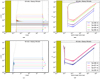 |
Fig. 3 Same as Fig. 2, but for the G0 and K0 stars, and glassy silicates. |
| In the text | |
|
Fig. 4 PR-drag pile-up scenario: evolution of β as a function of stellar distance r for the initially bound astrosilicate grains around the A0 star. The parent belt is located at 50 au (vertical dashed line), and the grains are released on increasingly eccentric orbits as β raises. The arrows represent the inital apoastron of the grains. |
| In the text | |
|
Fig. 5 Arrows representing the initial to final grain size evolution for a sample of simulations. The arrow head corresponds to the ejection size, or to total sublimation if it reaches the bottom of the figure. The colored rectangles are the range of grain sizes for which β > 0.5. |
| In the text | |
|
Fig. 6 PR-drag pile-up scenario: radial profiles for the size-integrated geometrical optical depth for all grain compositions and stellar types. |
| In the text | |
|
Fig. 7 Panels a–d: SED for each spectral type and all compositions in the PR-drag pile-up scenario. All spectra are normalized to the flux ratio at 2 μm, and compared to observed fluxes for exozodis around stars of similar type (for the F0 star, for which there is no available observed photometry at 2 μm, the valueis put to 1% of the stellar flux). Data points for Vega are from Absil et al. (2006), η Crv are from Lebreton et al. (2016), 10 Tau are from Kirchschlager et al. (2017), τ Cet are from Di Folco et al. (2007). Additional values are from Absil et al. (2013) and Mennesson et al. (2014). Panel e: SEDs for an A0 star and carbon grains, but only considering the flux within a radial distance indicated in the top right corner, and flux-normalized at λ = 2.12μm such that the disk flux amounts to 1.29% of the stellar flux at that wavelength (FLUOR excess for Vega). |
| In the text | |
|
Fig. 8 PR-drag pile-up scenario: flux level at 2 μm (left) and 10 μm (right) for an A0 star and carbon grains (top); and K0 star and astrosilicate grains (bottom). See Sect. 2.4 and Appendix C for the methodology. The vertical dashed line corresponds to the location of the sublimation radius rs as a function of grain size, while the full and dashed horizontal lines indicate the β = 0.5 and β = 1 limits, respectively. |
| In the text | |
|
Fig. 9 Panels a–c: grain size as function of the distance for all simulations run in the exocometary dust delivery at perihelion scenario (the yellow area, and the dotted and dash-dotted lines have the same meaning as in Fig. 2, while the dashed line corresponds to the limit between initially bound and unbound grains sizes). Panels d–f: specific case of an F0 star and carbon grains, for which the evolution of the grain size, the eccentricity, and the β value as a function of distance is displayed. In the case of eccentricity, the two curves overlap. |
| In the text | |
|
Fig. 10 Fraction of the surface mass loss for an exocomet orbiting an F0 star as a function of radial distance. The comet has an apoastron of 50 au, and an eccentricity of 0.994. Based on the comet evaporation prescription of Marboeuf et al. (2016, their Eq. (17)). |
| In the text | |
|
Fig. 11 Total geometrical optical depth (τ) in the exocometary dust delivery at perihelion scenario, assuming carbon grains. For illustrative purposes, a model with an exocomet perihelion larger than in the nominal case is shown for the F0 star. |
| In the text | |
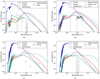 |
Fig. 12 Same as Fig. 7, but for the exocometary dust delivery at perihelion scenario. |
| In the text | |
|
Fig. 13 Contribution of each size and distance bin to the flux at 2 μm (left) and 10 μm (right) in the case of an F0 star and carbon grains. The grains are released by a exocomet at 0.13 au (top) and 1 au (bottom). |
| In the text | |
|
Fig. A.1 Top: evolution of the grain size as a function of the distance to the Sun for carbon grains of initial sizes 1, 3, 10, and 30 μm. Bottom: same, but for the glassy silicate. These plots reproduce the results presented in Fig. 5 of Krivov et al. (1998). |
| In the text | |
|
Fig. C.1 Cumulative time map derived from the simulations for the A0, carbon case. |
| In the text | |
|
Fig. C.2 Dominant physical processes driving the evolution of a grain as a function of the distance to the star and grain size. Shown are inward migration by PR-drag (red), sublimation (green), a combination of both (orange), and ejection by radiationpressure (blue) (see text for more details on how the dominant process is estimated). |
| In the text | |
|
Fig. C.3 Cumulative time map derived from the estimated timescales for the A0, carbon case. |
| In the text | |
Current usage metrics show cumulative count of Article Views (full-text article views including HTML views, PDF and ePub downloads, according to the available data) and Abstracts Views on Vision4Press platform.
Data correspond to usage on the plateform after 2015. The current usage metrics is available 48-96 hours after online publication and is updated daily on week days.
Initial download of the metrics may take a while.