| Issue |
A&A
Volume 569, September 2014
|
|
|---|---|---|
| Article Number | A81 | |
| Number of page(s) | 19 | |
| Section | Interstellar and circumstellar matter | |
| DOI | https://doi.org/10.1051/0004-6361/201423561 | |
| Published online | 26 September 2014 | |
APEX observations of supernova remnants
I. Non-stationary magnetohydrodynamic shocks in W44⋆,⋆⋆
1
Argelander Institut für Astronomie, Universität Bonn,
Auf dem Hügel, 71,
53121
Bonn,
Germany
e-mail:
This email address is being protected from spambots. You need JavaScript enabled to view it.
2
Univ. Grenoble Alpes, IPAG, 38000
Grenoble,
France
3
CNRS, IPAG, 38000
Grenoble,
France
4
LERMA, UMR 8112 du CNRS, Observatoire de Paris, École Normale Supérieure,
24 rue
Lhomond, 75231
Paris Cedex 05,
France
5
Max Planck Institut für Radioastronomie,
Auf dem Hügel 69,
53121
Bonn,
Germany
Received:
3
February
2014
Accepted:
22
July
2014
Abstract
Context. When supernova blast waves interact with nearby molecular clouds, they send slower shocks into these clouds. The resulting interaction regions provide excellent environments for the use of MHD shock models to constrain the physical and chemical conditions in these regions.
Aims. The interaction of supernova remnants (SNRs) with molecular clouds gives rise to strong molecular emission in the far-IR and sub-mm wavelength regimes. The application of MHD shock models in the interpretation of this line emission can yield valuable information on the energetic and chemical impact of SNRs.
Methods. New mapping observations with the APEX telescope in 12CO (3–2), (4–3), (6–5), (7–6), and 13CO (3–2) towards two regions in the SNR W44 are presented. Integrated intensities are extracted on five different positions, corresponding to local maxima of CO emission. The integrated intensities are compared to the outputs of a grid of models, which combine an MHD shock code with a radiative transfer module based on the large velocity gradient approximation.
Results. All extracted spectra show ambient and line-of-sight components as well as blue- and red-shifted wings indicating the presence of shocked gas. Basing the shock model fits only on the highest-lying transitions that unambiguously trace the shock-heated gas, we find that the observed CO line emission is compatible with non-stationary shocks and a pre-shock density of 104 cm-3. The ages of the modelled shocks scatter between values of ~1000 and ~3000 years. The shock velocities in W44F are found to lie between 20 km s-1 and 25 km s-1, while in W44E fast shocks (30–35 km s-1) as well as slower shocks (~20 km s-1) are compatible with the observed spectral line energy diagrams. The pre-shock magnetic field strength components perpendicular to the line of sight in both regions have values between 100 μG and 200 μG. Our best-fitting models allow us to predict the full ladder of CO transitions, the shocked gas mass in one beam as well as the momentum and energy injection.
Key words: ISM: supernova remnants / ISM: individual objects: W44 / ISM: kinematics and dynamics / shock waves / submillimeter: ISM / infrared: ISM
The velocity-integrated CO maps shown in Figs. 3 and 4 are available as FITS files at the CDS via anonymous ftp to cdsarc.u-strasbg.fr (130.79.128.5) or via http://cdsarc.u-strasbg.fr/viz-bin/qcat?J/A+A/569/A81
Appendix A is available in electronic form at http://www.aanda.org
© ESO, 2014
1. Introduction
Supernova explosions strongly affect the dynamical state of the interstellar medium (ISM). These explosions represent an injection of about 1051 erg into the ISM, immediately creating regions of very hot and tenous gas (e.g. Cox 2005). The shock waves originating from these explosions disperse molecular clouds and sweep up and compress the ambient medium (McKee & Cowie 1977). The evolution of the supernova remnant (SNR) can be described by four successive phases (Woltjer 1972): a free expansion phase, where the density of the ejected matter is much larger than that of the surrounding medium; a phase of adiabatic expansion, where the gas is too hot to undergo efficient radiative cooling; a radiative phase, where a dense, radiatively cooling shell of swept up gas is formed; and finally a fadeaway phase, when the shock wave has slowed down so much that it has turned into a sound wave.
If the supernova blast wave encounters ambient molecular clouds, it drives slower shocks into these clouds at a velocity that relates to the shock velocity in the intercloud medium via the density contrast between cloud- and intercloud gas (McKee & Cowie 1975). These slow shocks are similar to shocks originating in bipolar outflows of very young stars (e.g. Gusdorf et al. 2011): they strongly cool through molecular emission and can be observed in the far-IR and sub-mm wavelength regime (e.g. Neufeld et al. 2007; Frail & Mitchell 1998). Clear evidence of an interaction between a SNR and molecular clouds is typically provided by the detection of broad line wings, maser emission, highly excited far-IR CO, and near- and mid-infrared H2 emission (Reach et al. 2005). However, the modelling of these shocks differs from those associated with outflows in star forming cores because they are not irradiated by an embedded proto-star and they do not show any envelope or infall processes. The study of these interactions between SNRs and molecular clouds can yield valuable information on the supernova explosion and its impact on the surrounding medium. At the same time it can improve our understanding of the molecular clouds themselves. This information is needed for the understanding of various astrophysical questions, such as the energy balance of the ISM in galaxies, triggered star formation, and the origin and acceleration of cosmic rays.
High-J CO line emission is a very good diagnostic in this context because of the high abundance of CO in the molecular ISM, its important role for the cooling of the medium, and because its rotational transitions between higher energy levels are expected to trace shock conditions (e.g. Flower & Pineau des Forêts 2010; Meijerink et al. 2013). Here, we present new APEX CO observations towards two regions in one of the prototype interacting SNRs, W44, which has been the subject of many observational studies. We find MHD models compatible with our observations of CO emission and explore the consequences of the corresponding shock scenarios with respect to the impact of the SNR on its environment.
This paper builds on our previous study of MHD shocks based on high-J CO observations towards the SNR W28 (Gusdorf et al. 2012), but refines and extends the methods established there. The structure of the paper is as follows. In Sect. 2, we give a review of the SNR W44. In Sect. 3, we present our observations together with more detailed information on the observed regions W44E and W44F. Section 4 provides information on the molecular environment of W44. In Sect. 5, we show the CO maps observed towards both regions, while Sect. 6 focuses on the observed spectra towards the positions of our shock analysis. Our modelling approach with respect to the processing of observations and the grid of models is described in Sect. 7. In Sect. 8, the results are presented and discussed in Sect. 9. We summarize our findings in the concluding Sect. 10.
2. The supernova remnant W44
Observed lines, and associated frequencies, beam sizes, sampling, and forward efficiencies.
The region W44 (also known as G34.7–0.4, or 3C 392) is a prototype of the so-called mixed-morphology SNR as described by Rho & Petre (1998). This class refers to SNRs with centrally concentrated X-ray emission and a shell-like radio morphology. The size of this semi-symmetric SNR is about 30′ (Rho & Petre 1998). It is probably located in the Sagittarius arm (Castelletti et al. 2007) at the base of the Aquila supershell (Maciejewski et al. 1996) in a very obscured, complex region in the Galactic plane. Its distance has been estimated on the basis of HI 21 cm absorption measurements as ~3 kpc (Radhakrishnan et al. 1972; Caswell et al. 1975; Green 1989) and confirmed as 2.9 ± 0.2 kpc through molecular observations using the solar constants R0 = 7.6 kpc and Ω0 = 27.2 km s-1 kpc-1 (Castelletti et al. 2007). In this paper we use the distance value of 3 kpc as e.g. Abdo et al. (2010), Paron et al. (2009), and Seta et al. (2004). Based on this distance, the SNR’s size of ~30′ corresponds to ~26 pc. The SNR is believed to be in a radiative phase over much of its surface due to its estimated age of 2 × 10⁴ years (see below) and the observed cooling radiation (Cox et al. 1999; Chevalier 1999).
As first reported by Wolszczan et al. (1991), this type II SNR harbours a fast-moving 267 millisecond radio pulsar, PSR B1853+01, within the W44 radio shell, about 9′ south from its geometrical centre. Its progenitor is assumed to have had little influence on the parental molecular cloud on the scale of the SNR (Reach et al. 2005). The pulsar’s spin-down age amounts to 2 × 10⁴ years, while its distance, derived from the dispersion measure, is consistent with that of the SNR (Taylor & Cordes 1993). The pulsar wind powers a small synchrotron nebula observed in radio (Frail et al. 1996) and X-ray emission (Harrus et al. 1996; Petre et al. 2002).
The SNR W44 was first detected as a radio source already in the late 50s (Westerhout 1958; Mills et al. 1958; Edge et al. 1959) and identified as a possible SNR due to its non-thermal radio spectrum (Scheuer 1963). The shell-type shape in radio-continuum maps appears elongated from the north-east to the south-west, with a size of 25′× 35′ at 1442.5 MHz (Giacani et al. 1997) and enhanced radio emission at the eastern portion of the SNR. A high resolution VLA radio image at 1465 MHz, observed by Jones et al. (1993), reveals several filaments across the remnant and distortions along its eastern border. A plausible explanation for this feature could be the expansion of the SNR into a cloudy ISM, as already suggested by Velusamy (1988). Polarization measurements at 2.8 cm, conducted by Kundu & Velusamy (1972), show a high degree of polarization as large as 20%, possibly due to a highly regular oriented magnetic field, particularly over the main eastern and northern parts of the SNR. Based on earlier measurements between 22 MHz and 10 700 MHz, and new observations at 74 MHz and 324 MHz, Castelletti et al. (2007) derived a global integrated continuum spectral index −0.37 ± 0.02.
Observations of H i
reveal a fast, expanding shell-like structure at  and 210
km s-1 associated
with the SNR, corresponding to an expansion velocity of the H I shell of
and 210
km s-1 associated
with the SNR, corresponding to an expansion velocity of the H I shell of
 km s-1 (Koo & Heiles 1995). These authors estimated the H
I shell as being significantly smaller than the radio continuum shell. They interpreted this
double-shell structure as originating from the supernova exploding inside a pre-existing
wind bubble, whose shell constitutes the observed H I structure. Shelton et al. (1999) used a hydrocode model for W44 to show that this
interpretation is not compelling if the remnant’s evolution is taking place in a density
gradient, which leads to a spread in shell formation times for different parts of the
remnant’s surface. While Shelton et al. (1999)
assumed the ISM to be denser on the north-eastern, far side of the SNR, Seta et al. (2004) expected the strongest interaction
between the SNR and the ISM to occur in the front side of the SNR, while it is the
redshifted side that is visible as high-velocity expanding H I shell. This conclusion was
based on observed OH absorption corresponding to their component of “spatially extended,
moderately broad emission” in CO (1−0).
km s-1 (Koo & Heiles 1995). These authors estimated the H
I shell as being significantly smaller than the radio continuum shell. They interpreted this
double-shell structure as originating from the supernova exploding inside a pre-existing
wind bubble, whose shell constitutes the observed H I structure. Shelton et al. (1999) used a hydrocode model for W44 to show that this
interpretation is not compelling if the remnant’s evolution is taking place in a density
gradient, which leads to a spread in shell formation times for different parts of the
remnant’s surface. While Shelton et al. (1999)
assumed the ISM to be denser on the north-eastern, far side of the SNR, Seta et al. (2004) expected the strongest interaction
between the SNR and the ISM to occur in the front side of the SNR, while it is the
redshifted side that is visible as high-velocity expanding H I shell. This conclusion was
based on observed OH absorption corresponding to their component of “spatially extended,
moderately broad emission” in CO (1−0).
The centrally peaked X-ray morphology was first noted in observations from the Einstein Observatory Image Proportional Counter (IPC; Watson et al. 1983; Smith et al. 1985). Assuming the X-ray emission to be thermal (Szymkowiak 1980; Jones et al. 1993), the morphology of the emission was explained by a scenario where a possible X-ray shell is unseen because it has become too cold to be detected through the intervening ISM (Smith et al. 1985; Jones et al. 1993). Observations with the ROSAT Position Sensitive Proportional Counters (PSPC; Rho et al. 1994) confirmed the centrally peaked X-ray morphology and revealed a largely uniform temperature over the remnant. Rho et al. (1994) as well as Jones et al. (1993) interpreted this observation using an evaporation model with a two-phase ISM structure of clump and interclump gas (White & Long 1991), where the material stemming from evaporating clouds increases the density of the SNR interior. More recent models stressed the important role of thermal conduction in the creation of the centrally peaked X-ray emission (Cox et al. 1999; Kawasaki et al. 2005). Thermal conduction levels out gradients of temperature in the hot interior plasma while pressure equilibrium then yields a higher density at the centre. Once the forward shock velocity has decreased so that the X-ray emission from the shell becomes too soft to pass through the ISM, the centrally brightened X-ray emission appears.
Probably as a result of the interaction between the SNR and a molecular cloud, the eastern limb shows a lack of X-ray emission within the radio shell, while weaker diffuse X-ray emission extends up to the northern radio boundary of W44 (Giacani et al. 1997). The existence of a non-thermal X-ray component was shown by Harrus et al. (1996) when they detected a hard X-ray source coincident with the position of the pulsar region interpreted as an X-ray synchrotron nebula.
The first detection of optical filaments in Hα and [S II] images of W44, seen in the north-eastern and south-eastern parts, was reported by Rho et al. (1994). These filaments are mainly confined within the X-ray emitting region and are absent in the eastern region. Along the north-west border of the remnant, there is excellent correlation between optical and radio emission at 1.4 GHz, suggesting that radiative cooling of the shocked gas immediately behind the shock front, where enhanced magnetic fields are present, is the origin of the optical radiation (Giacani et al. 1997).
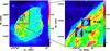 |
Fig. 1 Location of the fields covered by our CO observations on the larger-scale radio continuum image at 1442.5 MHz, taken from Giacani et al. (1997). The wedges indicate the intensity of the continuum in Jy/beam. Left panel: entire SNR, right panel: zoom in the regions W44E and W44F. The inserts show the distribution of the CO (6–5) emission, integrated between 20 km s-1 and 70 km s-1, for which the colourscale is in the range 0–50 K km s-1, and the contours are radio continuum in steps of 10 mJy. The size of the zoombox is ~10.3 × 12.4 pc. |
The association of molecular gas with W44 was already reported by Dickel et al. (1976), who attributed the flattened shell structure of the SNR to an encounter with a dense molecular cloud. Wootten (1977) observed a broadening of line widths and an intensification of line strength in CO (1–0), which he explained by the heating and compression of the ISM by the SNR. Denoyer (1983) questioned the shock processing of the adjacent molecular cloud, referring to an absence of chemical shock characteristics and the possible explanation of broadened lines by overlapping line components along the line of sight. However, subsequent observations of emission from shock-tracing molecules and fine-structure line emission (Seta et al. 1998; Reach & Rho 1996, 2000; Reach et al. 2005; Neufeld et al. 2007; Yuan & Neufeld 2011) as well as OH maser emission (Claussen et al. 1997; Hoffman et al. 2005) have removed doubts about the existence of an interaction with a molecular cloud.
Finally, W44 is an important site for the study of cosmic-ray production, acceleration, and propagation based on the observations of γ-rays stemming from the interaction of cosmic-rays and the ISM. These interactions include high-energy electron bremsstrahlung and inverse Compton scattering of the leptonic cosmic-ray component as well as proton-proton collisions of the hadronic component creating neutral pions, whose decay generates γ-rays. A first detection in the GeV regime was achieved with the EGRET instrument aboard the Compton Gamma Ray Observatory, although an association with W44 was not clear (Esposito et al. 1996). The Fermi Large Area Telescope (LAT) detected a source morphology corresponding to the SNR radio-shell at energies above 200 MeV (Abdo et al. 2010). Modelling the observed emission, these authors concluded that neutral pion decays are plausibly responsible for the emission, although a bremsstrahlung scenario could not be ruled out completely. Giuliani et al. (2011) subsequently excluded leptonic emission as the main contribution based on observations at lower energies (30 MeV–50 GeV) using the AGILE instrument. They reported direct evidence of pion emission based on a steep decline of the spectral energy distribution below 1 GeV. Ackermann et al. (2013) presented observations in the sub-GeV part of the γ-ray spectrum, obtained within four years with the Fermi/LAT, from the compact regions delineated by the radio continuum emission. Based on the observation of the characteristic pion-decay feature in their spectrum (“pion-decay bump”) they could finally provide direct evidence of the acceleration of cosmic-ray protons.
3. Observations
In this section, we introduce the observed regions, W44E and W44F, and present our observations of CO and 13CO species performed with APEX1 telescope (Güsten et al. 2006). In Table 1, we provide observing parameters associated with each observed line (frequencies, beam sizes, corresponding sampling, and forward efficiencies).
3.1. W44E
3.1.1. Region
As displayed in Fig. 1, W44E lies in the
north-eastern flattened part of the radio shell, where the SNR is interacting with the
densest part of the molecular cloud (Wootten
1977). Eastern of this region, Seta et al.
(2004) located an “edge” in CO (1–0) emission, where the CO intensity drops by
a factor of ~2 and the
emission lines are broadened and velocity-shifted with respect to the emission outside
the SNR. They attribute this morphological feature to the interaction of the SNR with a
clumpy molecular cloud, referring to the model of Chevalier (1999), where a radiative shell formed in the diffuse interclump gas
drives slow molecular shocks into the clumps. The interaction between the giant
molecular cloud and the SNR is believed to take place on the front side of the remnant
as OH absorption is detected (Reach & Rho
1998). The drop in molecular column density is then attributed to dissociation
of molecules and evaporation of molecular mass. Seta et
al. (2004) did not detect wing emission towards W44E in CO (1–0), defined as
lines with full velocity widths greater than 25 km s-1. Wing emission was however
detected in CO (3–2) by Frail & Mitchell
(1998) and in CO (2–1) by Reach & Rho
(2000) and Reach et al. (2005). Both
lines show a narrow component, tracing the unshocked gas also visible in 13CO (FWHM ~ 5
km s-1, centred
at ~45 km s-1), and a broad component
(FWHM ~
30 km s-1) tracing the shocked gas. Combining these observations
with infrared spectroscopy, Reach & Rho
(2000) concluded to the existence of different shocks into moderate
(~102 cm-3) and high-density
(~104 cm-3) environments. In that
picture, bright H emission
together with emission of CO requires higher density gas residing in clumps that
survived the initial blast wave. In a similar manner, Neufeld et al. (2007) identified five different groups of emission features
towards W44E, classified on the basis of their spatial distribution. The pure rotational
lines of H (J>
2), together with lines of sulfur, constituted one of these groups,
likely originating in molecular material subject to a slow, nondissociative shock.
emission
together with emission of CO requires higher density gas residing in clumps that
survived the initial blast wave. In a similar manner, Neufeld et al. (2007) identified five different groups of emission features
towards W44E, classified on the basis of their spatial distribution. The pure rotational
lines of H (J>
2), together with lines of sulfur, constituted one of these groups,
likely originating in molecular material subject to a slow, nondissociative shock.
Observed lines and corresponding telescope parameters – the case of W44E.
Observed lines and corresponding telescope parameters – the case of W44F.
In addition to the broad CO line emission, the observed
H emission, and
atomic fine structure lines, the existence of OH maser emission constitutes another
strong indication of an interaction between the SNR and a molecular cloud. Claussen et al. (1997) detected ten OH maser features
at 1720 MHz in W44E, two of them were shown to have multiple angular components (Hoffman et al. 2005). The masers appear along the
continuum edges of the synchrotron emission. Claussen et
al. (1997) interpret this region of enhanced synchrotron emission as featuring
particle acceleration in a shock, referring to Blandford
& Eichler (1987). However, the enhancement could also be explained
without the claim of new particle acceleration, originating from the compression of the
magnetic field and pre-existing relativistic electrons (Blandford & Cowie 1982; Frail
& Mitchell 1998). The velocities of the masers have a low dispersion
(<1 km s-1) around a mean value of
 km s-1, which agrees very well with
the systemic velocity of W44E of
km s-1, which agrees very well with
the systemic velocity of W44E of  km s-1. The explanation for this
low dispersion was given in terms of tangential amplification (Frail et al. 1996): the maser emission is only seen where the
acceleration of the gas is transverse to the line of sight. From the strong inversion of
the OH (1720 MHz) line through collisions with H, possible
excitation conditions can be inferred: kinetic temperatures should lie between 25 K
≤Tk ≤ 200 K,
while the density is expected to be 10
km s-1. The explanation for this
low dispersion was given in terms of tangential amplification (Frail et al. 1996): the maser emission is only seen where the
acceleration of the gas is transverse to the line of sight. From the strong inversion of
the OH (1720 MHz) line through collisions with H, possible
excitation conditions can be inferred: kinetic temperatures should lie between 25 K
≤Tk ≤ 200 K,
while the density is expected to be 10 cm-3 ≤
nH2 ≤ 105
cm-3 (Elitzur 1976). Lockett et al. (1999) derived tighter physical conditions in the region, as
they constrained a kinetic temperature of 50 K ≤Tk≤ 125 K, a molecular hydrogen density of
10
cm-3 ≤
nH2 ≤ 105
cm-3 (Elitzur 1976). Lockett et al. (1999) derived tighter physical conditions in the region, as
they constrained a kinetic temperature of 50 K ≤Tk≤ 125 K, a molecular hydrogen density of
10 cm-3, and OH
column densities of ~1016 cm-2. Frail &
Mitchell (1998) presented a map in CO (3–2) towards W44E, where they show that
the masers delineate the forward edge of molecular gas, preferentially located nearer to
the edge of the shock (as traced by the non-thermal emission) than the peak of CO. They
report a correlation between the integrated CO (3–2) maps and the radio continuum.
cm-3, and OH
column densities of ~1016 cm-2. Frail &
Mitchell (1998) presented a map in CO (3–2) towards W44E, where they show that
the masers delineate the forward edge of molecular gas, preferentially located nearer to
the edge of the shock (as traced by the non-thermal emission) than the peak of CO. They
report a correlation between the integrated CO (3–2) maps and the radio continuum.
The line-of-sight magnetic field strength B∥ in the region was determined by Claussen et al. (1997) to be within a factor of 3 of 0.2 mG (with the expectation value of the total magnetic field given as B = 2B∥) in all maser locations using Zeeman splitting between the right- and left-circularly polarized maser lines in OH (1720 MHz). They found the direction of the field throughout the remnant to be constant. Hoffman et al. (2005) constrained the strength of the magnetic field as ~1 mG on the basis of MERLIN and VLBA circular polarization observations of OH maser lines. The position angle of the magnetic field based on linear polarization of the masers aligns with the direction of the shocked dense gas filament.
3.1.2. Data
Observations towards the region W44E were conducted in July 2010. We made use of a
great part of the suite of heterodyne receivers available for this facility:
FLASH3452, FLASH460 (Heyminck et al. 2006), and CHAMP+ (Kasemann et al. 2006; Güsten et al.
2008), in combination with the MPIfR Fast Fourier Transform Spectrometer
backend (FFTS, Klein et al. 2006), or with the
newly commissioned MPIfR X-Fast Fourier Transform Spectrometer backends (XFFTS, Klein et al. 2012). The central position of all the
observations was set to be (α[ J2000 ] = 18h56m28 40, β[ J2000 ] =
01°29′59
40, β[ J2000 ] =
01°29′59  0). Focus was checked at the beginning of each observing session, after sunrise and/or
sunset on Mars, Jupiter, or Saturn. Continuum and CO line pointing was locally
established on G34.26 and R-Aql. The pointing accuracy was found to be of the order of
5′′ rms,
regardless of the receiver that was used. Table 2
contains the main characteristics of the telescope, and of the observing set-up for each
observed transition: used receiver, corresponding observing days, beam efficiency,
system temperature, and spectral resolution. The observations were performed in
position-switching/raster mode using the APECS software (Muders et al. 2006). The data were reduced with the CLASS software3.
0). Focus was checked at the beginning of each observing session, after sunrise and/or
sunset on Mars, Jupiter, or Saturn. Continuum and CO line pointing was locally
established on G34.26 and R-Aql. The pointing accuracy was found to be of the order of
5′′ rms,
regardless of the receiver that was used. Table 2
contains the main characteristics of the telescope, and of the observing set-up for each
observed transition: used receiver, corresponding observing days, beam efficiency,
system temperature, and spectral resolution. The observations were performed in
position-switching/raster mode using the APECS software (Muders et al. 2006). The data were reduced with the CLASS software3.
3.2. W44F
3.2.1. Region
The W44F region lies south-eastern of W44E and hosts a thin filament of gas ranging from the north-west to the south-east, aligned with the radio continuum contours (see Fig. 1). According to the radio continuum emission, the long axis of the filament seems to be parallel to the shock front. Claussen et al. (1997) detected three OH 1720 MHz masers in this region with an average velocity of 46.6 km s-1. In the CO (3–2) map of Frail & Mitchell (1998), the masers border the northern CO emission peak integrated over the red-shifted spectral wing between 49 km s-1 and 60 km s-1. The spectrum in CO (3–2) they observed towards W44F has a double-peak structure with peaks at 39 km s-1 and 50 km s-1. This double-peak structure is also visible in the spectrum of CO (2–1) (Reach et al. 2005). Although this could possibly be interpreted as a superposition of two moderately broad components in the line of sight, the deep trough’s alignment with the peak in the 13CO (1–0) spectrum they also observed reveals that it actually is broad-line emission being absorbed by cold, narrow foreground gas. The magnetic field strength was also measured in W44F using Zeeman splitting between the right- and left-circularly polarized maser lines in OH (1720 MHz) (Frail & Mitchell 1998; Hoffman et al. 2005). The results were the same as in W44E, as well as the orientation of the position angle of the magnetic field being aligned with the filament of shocked gas.
3.2.2. Data
Observations towards the region W44F were conducted in several runs in the year 2009
(in June and August), and also in July 2012 (for 13CO (3–2)). The central
position of all the observations was set to be (α[ J2000 ] =
18h56m36 9, β[ J2000 ] =
01°26′346).
Focus was checked at the beginning of each observing session, after sunrise and/or
sunset on Mars, Jupiter, or Saturn. Continuum and line pointing was locally checked on
G34.26 and R-Aql. The pointing accuracy was found to be of the order of 5′′ rms, regardless of the
receiver that was used. Table 3 contains the same
parameters as Table 2, for observations of W44F.
The observations were performed in position-switching/raster mode using the APECS
software (Muders et al. 2006). The data were
reduced with the CLASS software4.
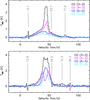 |
Fig. 2 CO spectra (in TMB) averaged over the W44E (top) and W44F (bottom) regions. The spectra correspond to the transitions of CO (3–2) (black), CO (4–3) (pink), CO (6–5) (blue), and CO (7–6) (light blue). The CO spectral resolutions are 2.18 km s-1 for CO (7–6) in W44F, and 1.0 km s-1 for all other lines. |
4. Averaged CO emission towards W44E and W44F
The SNR W44 is surrounded by several molecular clouds. To understand the CO emission
towards W44E and W44F we have averaged all spectra obtained in each mapped region
respectively, after convolving them to a common spatial resolution of
 , that of our CO (3–2) observations. These
averaged spectra are shown in Fig. 2. The value for the
systemic velocity of W44 that we found in the literature is 45 km s-1 (e.g. Claussen et al. 1997). The peaks of our spectra agree with this value. In
the averaged spectra of W44F we detect strong absorption between ~40 km s-1 and ~50 km s-1 in all transitions up to CO
(6–5), which is attributed to absorption by cold foreground gas.
, that of our CO (3–2) observations. These
averaged spectra are shown in Fig. 2. The value for the
systemic velocity of W44 that we found in the literature is 45 km s-1 (e.g. Claussen et al. 1997). The peaks of our spectra agree with this value. In
the averaged spectra of W44F we detect strong absorption between ~40 km s-1 and ~50 km s-1 in all transitions up to CO
(6–5), which is attributed to absorption by cold foreground gas.
Seta et al. (1998, 2004) have studied the vicinity of W44 in CO (1–0) and CO (2–1). In their earlier
paper, presenting observations at low spatial resolution5, they divided the CO emission towards W44 into three velocity components at
 km
s-1, 30–65 km
s-1, and 70–90 km
s-1. The 13 km
s-1 component
corresponds to well-known foreground clouds in the solar neighbourhood, in earlier
publications attributed to the dust cloud Khavtassi3 at 15 km s-1 (Knapp & Kerr 1974; Wootten 1977;
Scoville et al. 1987). We detect this component
clearly in CO (3–2) towards both regions, although towards W44F it is mostly seen in
absorption. In both fields, this component is rather spatially uniform, although towards
W44E the intensity of this feature increases in the south-eastern direction.
km
s-1, 30–65 km
s-1, and 70–90 km
s-1. The 13 km
s-1 component
corresponds to well-known foreground clouds in the solar neighbourhood, in earlier
publications attributed to the dust cloud Khavtassi3 at 15 km s-1 (Knapp & Kerr 1974; Wootten 1977;
Scoville et al. 1987). We detect this component
clearly in CO (3–2) towards both regions, although towards W44F it is mostly seen in
absorption. In both fields, this component is rather spatially uniform, although towards
W44E the intensity of this feature increases in the south-eastern direction.
The 70–90 km s-1 component was attributed to clouds behind W44 with an uncertain fraction of emission from accelerated gas from W446. The integrated spectrum in CO (3–2) towards W44E shows a weak peak at 78 km s-1 that might corresponds to cloud 10 (CO G34.7–0.1, ν= 78 km s-1) in the labelling of Seta et al. (1998), although the spatial distribution of the emission is difficult to disentangle from highly red-shifted shocked gas. Towards W44F we notice a broad emission feature in the velocity regime between 70 km s-1 and 90 km s-1 in CO (3–2), peaking at 72 km s-1, together with a narrow peak at 86 km s-1 that is also seen in absorption in CO (4–3). Both features appear spatially uniform over the observed field.
The 30–65 km s-1 component is considered to be associated with W44. Towards W44E this central component appears even broader in our data (15–70 km s-1), and also towards W44F the wings seem to stretch farther. Seta et al. (1998) identified six molecular clouds in this velocity range, of which three are candidates for an interaction (given their spatial coincidence with the SNR and similar estimated radial velocities) and one that is probably interacting with W44 (G34.8–0.6, ν= 48 km s-1), showing increased line widths and an abrupt shift in radial velocity at the rim of the SNR. At 54 km s-1 we detect another emission peak towards W44E, which could correspond to the absorption dip towards W44F at 54.5 km s-1. The emission at this velocity is strongly spatially varying. Its intensity increases towards the south of W44E, where it becomes comparable in intensity to the main peak. The origin might be a confined clump of material moving within the molecular cloud.
5. CO maps
5.1. CO maps towards W44E
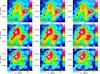 |
Fig. 3 Overlays of the velocity-integrated maps of CO (3–2) (left
column), CO (4–3) (middle column), and CO (7–6)
(right column) as white contours on the CO (6–5) emission (colour
background) observed towards W44E with the APEX telescope. The maps are in their
original resolution (9 |


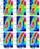 |
Fig. 4 Same as Fig. 3 but observed towards W44F. The black and blue hexagons mark the positions of the OH masers observed by Claussen et al. (1997) and Hoffman et al. (2005). |
Positions of our analysis.
Figure 3 shows maps of integrated CO emission in CO (6–5) with contours of integrated CO (3–2), (4–3), and (7–6) (respectively 1st, 2nd, and 3rd column) emission overlayed towards W44E, for the blue wing (top row, 20–40 km s-1), the red wing (bottom row, 50–70 km s-1), and the ambient velocity regime (central row, 40–50 km s-1). The positions of OH masers detected towards W44E are also displayed. The lower integration boundary of the blue wing of 20 km s-1 was chosen to avoid the contribution of the foreground cloud at ~13 km s-1 in CO (3–2). Similarly we chose the upper integration boundary of the red wing as 70 km s-1 because at higher velocities the contribution of red-shifted gas related to W44 and background cloud emission reported by Seta et al. (1998) is difficult to disentangle.
The emission distribution peaks in all CO maps behind or near the line of masers, which trace the shock front moving eastward into the ambient molecular gas (Claussen et al. 1997). The eastern peak exhibits strong wings towards higher and lower velocities relative to the systemic velocity of W44. There is another emission peak towards the interior of W44 close to the second masering region distinct from the delineated masers to the east. This peak is mostly seen in the blue-shifted velocity regime. Here the spatial displacement between maser and CO emission is less clear than for the other peak.
For our shock analysis, we aimed at choosing positions of clearly shocked gas, defined as positions of maximum CO emission in a given velocity range for a maximum number of observed transitions. Therefore we first determined the local maxima of CO emission in all of our transition maps in the various velocity regimes and then chose the positions of our analysis based on these maxima. In the centre panel of Fig. 5, we show the two positions resulting from this procedure: the one close to the line of masers tracing the outer shock front (black circle, denoted as W44E1) and the one towards the interior (blue circle, denoted as W44E2). The coordinates of W44E1 and W44E2 are listed in Table 4.
5.2. CO maps towards W44F
The corresponding maps of integrated CO emission for the three velocity regimes towards W44F, together with observed maser positions, are shown in Figure 4. The maps in the ambient velocity regime (central row) in CO (3–2) and CO (4–3) have to be treated with some caution as they suffer from substantial absorption in the line centres, as can e.g. be seen in Fig. 2 and Fig. 6. In all velocity regimes, a thin filament of gas from the north-west to the south-east of the maps can be traced. Only the convolved map of CO (7–6) does not show such a clear filament in the blue velocity regime. The extent of the filament stretches farther to the south for the blue wing emission than for the red wing. Again, we defined the position of clear shock interaction as showing maximum CO emission in a given velocity range for a maximum number of observed transitions. Accordingly, based on the local maxima of CO emission in all our transition maps, we selected three positions in W44F for our modelling analysis. These positions are displayed in the central panel of Fig. 6. The first position in the north covers the maser locations observed by Claussen et al. (1997) and Hoffman et al. (2005). It is particularly prominent in the redshifted velocity regime (northern black circle in Fig. 6, denoted as W44F1). There is another maximum in the red wing regime (southern black circle in Fig. 6, denoted as W44F2), while the emission integrated over the blue wing peaks still farther to the south (blue circle in Fig. 6, denoted as W44F3). The corresponding coordinates are listed in Table 4.
6. Individual spectra of 12CO and 13CO
6.1. Positions of analysis in W44E
The individual spectra towards our positions of analysis in W44E, as shown in Fig. 5, exhibit a complex structure. In CO (3–2), two components are seen as already observed by Frail & Mitchell (1998), Reach & Rho (2000), and Reach et al. (2005) in CO (3–2) and CO (2–1): there is a narrow component tracing the cold ambient gas and a broad component due to emission from shocked gas.
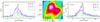 |
Fig. 5 Central Panel: positions of our analysis in W44E (W44E1: black
circle, W44E2: blue circle) on the velocity-integrated CO (6–5) emission
( |

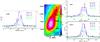 |
Fig. 6 Same as Fig. 5 but towards W44F. The positions in the central panel are W44F1, W44F2, and W44F3 (north to south). Left panel: spectra observed in the position W44F3. Right panel: spectra observed in the position W44F1 (top) and W44F2 (bottom). The CO spectral resolutions are 2.18 km s-1 for CO (7–6) and 1.0 km s-1 for all other lines. |
Towards W44E1, the emission of the cold quiescent gas in 13CO (3–2) is confined between 40 km s-1 and 50 km s-1 showing two components: one centred at 44.5 km s-1 with a FWHM of 5.2 km s-1 and another very narrow component (FWHM = 1 km s-1) at 45.6 km s-1. The FWHM of the former component is identical to the FWHM determined by Reach et al. (2005) for the central peak in CO (2–1) and its central velocity is close to the average OH (1720 MHz) maser velocity of 44.7 km s-1. The emission in 13CO aligns with the central, narrow peak in our spectrum of 12CO (3–2), although probable self-absorption renders the determination of the FWHM of the peak of the latter difficult. The lines in CO (4–3), (6–5), and (7–6) show self-absorption features in the range between 43 km s-1 and 46 km s-1. The shock-broadened lines are asymmetric but similar in shape among all transitions. The red-shifted wings of the lines extent to high velocities at weak levels of emission, reaching well beyond the velocity regime of 30–65 km s-1 considered to be associated with W44 by Seta et al. (1998).
Towards W44E2, the cold gas traced by 13CO (3–2) exhibits only one component centred at 44.8 km s-1 with an FWHM of 3.2 km s-1. This cold ambient component is also visible as a narrow peak in the spectrum of 12CO (3–2) at 44.6 km s-1. The shape of the shock-broadened line component is again similar in all transitions. Other than in W44E1, the main peak of the shock emission is slightly offset from the ambient emission at ~38 km s-1. Furthermore, two shoulders can be identified, one in the blue- and one in the red-shifted velocity regime, the latter again stretching out to very high velocities of 80–90 km s-1.
Figure 7 shows the spectra of 12CO (3–2) and 13CO (3–2) towards W44E1 and W44E2 (two top panels, left ordinate), resampled to a common spectral resolution of 1 km s-1. The line temperature ratio of 12CO (3–2)/13CO (3–2) (right ordinate) is displayed in the lower velocity shift’s regime, where 13CO is detected at more than 2σ (orange dots) and 3σ (red dots). Because these signal-to-noise values are only reached for 13CO towards the centres of the 12CO lines, the optical thickness values can accordingly only be inferred at the inner parts of the 12CO line wings. There, the line ratios yield optical thickness values of 3–7, assuming a typical interstellar abundance ratio of 50–60 (e.g. Langer & Penzias 1993). The line temperature ratio towards W44E at ~13 km s-1, corresponding to foreground emission, yields optical thickness values of 3–14 in this component. We note that this analysis relies on the assumption of an equal excitation temperature for both isotopologues.
6.2. Positions of analysis in W44F
As already observed by Frail & Mitchell (1998) and Reach et al. (2005), the low velocity emission towards W44F seems to be absorbed by foreground gas in the lower transitions of CO. This effect is also present in our data, although additional absorption is caused by emission in our reference position. Compared to W44E, the shock emission appears narrower with FWHM less than 45 km s-1 and with the lines being more symmetric.
Towards W44F1, the quiescent gas as visible in 13CO (3–2) peaks at 46 km s-1 with an FWHM of 7.8 km s-1 (see Fig. 7), which agrees with the average OH (1720 MHz) maser velocity of 46.6 km s-1. Absorption is seen in all transitions to various extents in the lines of 12CO, the lowest transitions being affected in the full range between 39.5 km s-1 and 50 km s-1. This is similar for W44F2, while there the emission of 13CO (3–2) shows a double-peaked structure with a broader component at 45.7 km s-1 (FWHM 6.7 km s-1) and a narrow component at 46.4 km s-1 (FWHM 0.7 km s-1). In W44F3, the narrow ambient component disappears again, the remaining component being centred at 44.4 km s-1 with an FWHM of 7.2 km s-1. W44F3 shows the most asymmetric profiles with a shoulder in the red-shifted wing (as visible in CO (6–5)) and pronounced emission in the blue wing.
The line temperature ratio of 12CO (3–2)/13CO (3–2) towards W44F in the lower velocity regime, where 13CO is detected at more than 2σ (orange dots) and 3σ (red dots) is displayed in Fig. 7 (three bottom panels, right ordinate). As in W44E, the ratios yield optical thickness values of 3–7 in the wings.
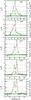 |
Fig. 7 Spectra (in TMB) of 12CO (3–2) (grey, left ordinate) and 13CO (3–2) (green, left ordinate) together with the line temperature ratio of 12CO (3–2)/13CO (3–2) (dots, right ordinate). The ratio is shown for 13CO (3–2) line temperatures higher than 2σ (orange dots) and 3σ (red dots). Grey dotted lines indicate values of the temperature ratio as displayed on the left-hand side of these lines. The positions displayed are W44E1 and W44E2, and W44F1, W44F2, and W44F3 (top to bottom). The corresponding values of the optical thickness in the line wings are in the range of 3–7. |
7. Modelling
7.1. The observations
As described in Sect. 6, all spectra we have extracted towards our five positions of maximum CO emission in W44E and W44F show broad line wing emission around a central velocity consistent with the cold ambient gas. Most likely these profiles arise from a superposition of different shock components propagating into the dense gas of molecular clumps, which are nearly impossible to disentangle. In order to still get significant constraints on the dominant shock features and environmental conditions, we separated the profiles into a blue and a red lobe and applied our shock analysis to each of these velocity domains independently.
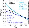 |
Fig. 8 Rotational diagram of the blue shock component in W44E2. Observations are marked by black squares. The lines show the C-type (dark blue) and CJ-type (light blue) shocks that yield the best fits to the CO (7–6) and (6–5) transitions. |
All line profiles, convolved to a common angular resolution of
18 , were fitted using a combination of
up to four independent Gaussians with fully adjustable parameters. In W44E, these free
fits yielded similar fit components for all transitions: two Gaussians in W44E1 and three
in W44E2 with one additional ambient component in CO (3–2). In W44F, the fitting procedure
was hindered by the deep absorption of the line centres. Therefore the fits for the CO
(3–2) and CO (4–3) spectra could only be based on information from the wings, starting
with initial values for the fitting procedure as obtained from the higher transitions.
However, large uncertainties result from the lack of information for the fit of these
lines. To handle this problem, we decided not to use the information of the line centres
based on these fits, but rather to utilise the similar shape of emission lines among all
transitions as observed in W44E. In particular, the ratio between the velocity-integrated
intensities of the full lobe and the velocity-integrated intensities of only the wings
turned out to be constant among all transitions within ±5% in W44E. Assuming a similar behaviour in
W44F, we used this ratio derived from the CO (6–5) and CO (7–6) spectra to obtain
estimations for the full-lobe integrated intensities in CO (3–2) and CO (4–3) based on
their wing emission.
, were fitted using a combination of
up to four independent Gaussians with fully adjustable parameters. In W44E, these free
fits yielded similar fit components for all transitions: two Gaussians in W44E1 and three
in W44E2 with one additional ambient component in CO (3–2). In W44F, the fitting procedure
was hindered by the deep absorption of the line centres. Therefore the fits for the CO
(3–2) and CO (4–3) spectra could only be based on information from the wings, starting
with initial values for the fitting procedure as obtained from the higher transitions.
However, large uncertainties result from the lack of information for the fit of these
lines. To handle this problem, we decided not to use the information of the line centres
based on these fits, but rather to utilise the similar shape of emission lines among all
transitions as observed in W44E. In particular, the ratio between the velocity-integrated
intensities of the full lobe and the velocity-integrated intensities of only the wings
turned out to be constant among all transitions within ±5% in W44E. Assuming a similar behaviour in
W44F, we used this ratio derived from the CO (6–5) and CO (7–6) spectra to obtain
estimations for the full-lobe integrated intensities in CO (3–2) and CO (4–3) based on
their wing emission.
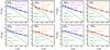 |
Fig. 9 Best-model comparisons between CO observations and models for all positions in W44E (W44E1: top row, W44E2: bottom row) for both the blue and red shock components, respectively. The four panels on the left show the high velocity fits while the four panels on the right show the low velocity fits in each position. Observations are marked by black squares, the best-shock models are displayed in violet line (blue lobe) and orange line (red lobe) and diamonds, the CO layer that we used to compensate the ambient emission affecting the CO (3–2) and CO (4–3) transitions in green line and triangels, and the sum of ambient and shock component in blue line (blue lobe) and red line (red lobe) with circles. |
The integration intervals were determined according to our knowledge of the ambient cloud component, based on the fits of 13CO (3–2) emission. To access the uncertainty of the lobe-separation with respect to the ambient velocity component, we varied the upper limit of the blue and the lower integration limit of the red lobe within the FWHM of the 13CO (3–2) fit. The integration intervals for our five positions are listed in Tables 6 and 8. The errors in the integrated intensities in the CO (3–2) and CO (4–3) transitions in W44F, which were estimated based on the integrated intensities in the wings, were determined by varying the assumed lobe-wing integrated intensity ratio by ±10%. For the final plot of the velocity-integrated intensities of all CO lines against the rotational quantum number of their upper level (so-called spectral line energy distribution), we also accounted for the filling factor of the lines, which is assumed to be the same for all transitions in each position, once the maps have all been convolved to the same resolution. We based these estimations on the half-maximum contours in the maps of CO (6–5), which provides high angular resolution, has a good signal-to-noise ratio, and which is barely affected by self-absorption. We note however that a reliable estimate of these factors would require high-resolution interferometric observations of the analysed regions, which have not been performed so far. In ambiguous cases we examined various values of the filling factor within our analysis. The final values we obtained are listed in Tables 6 and 8. To account for possible errors in the filling factor, we varied its value by ±0.1.
The errors in the integrated line intensities due to uncertainties in the integration
intervals and due to assumed filling factors were combined with the errors resulting from
the inherent rms noise fluctuations of the profiles and the uncertainties in subtracting
baselines as described by Elfhag et al. (1996).
This results in a total error in the integrated line intensities,
![Mathematical equation: \begin{eqnarray} \Delta I &=& \sqrt{\Delta I_{\rm line}^2+\Delta I_{\rm base}^2+\Delta I_{\rm integration}^2+\Delta I_{\rm FF}^2}\\[3mm] &=& \sqrt{\frac{\sigma}{\sqrt{N}}\cdot B \sqrt{\frac{\Delta \varv}{B-\Delta \varv}}+\Delta I_{\rm integration}^2+\Delta I_{\rm FF}^2} , \end{eqnarray}](/articles/aa/full_html/2014/09/aa23561-14/aa23561-14-eq71.png) where
Δν (km s-1) is the total velocity width
of the spectral line, N is the total number of spectrometer channels
covering a total velocity range of B km s-1, and σ is the r.m.s noise per channel.
where
Δν (km s-1) is the total velocity width
of the spectral line, N is the total number of spectrometer channels
covering a total velocity range of B km s-1, and σ is the r.m.s noise per channel.
As can be seen in the rotational diagrams displayed in Figs. 9 and 10, the large errors in the column densities of the upper levels of the (4–3) and (3–2) transitions in W44F mirror the uncertainties in the flux reconstruction necessary in order to account for the absorption in the line centre. The errors in the spectral line energy distributions and the rotational diagrams, respectively, are larger in W44F than in W44E because in W44E the ratio between flux in the line wings and flux in the line centre is higher, such that the uncertainty due to the unknown value of the ambient velocity is of less consequence.
7.2. The models
For the interpretation of the observed spectral energy distributions (SLEDs), we used a combined model consisting of a one-dimensional, plane-parallel shock model and a radiative transfer module (Gusdorf et al. 2008, 2012). The former model solves the magneto-hydrodynamical equations in parallel with a large chemical network (including more than 100 species linked by over 1000 reactions) for stationary C- and J-type shocks (Flower & Pineau des Forêts 2003; Flower et al. 2003) or approximated non-stationary CJ-type shocks. The theoretical elements for the computing of approximated, non-stationary shock models have been introduced in Chieze et al. (1998) and Lesaffre et al. (2004a,b). They have been proven useful mostly in the interpretation of H2 pure rotational lines observed in shocks associated with bipolar outflows that accompany star formation, (e.g. Giannini et al. 2004; Gusdorf et al. 2008, 2011) and associated with SNRs (e.g. Cesarsky et al. 1999).
The radiative transfer of H as the main gas
coolant is self-consistently calculated for the first 150 ro-vibrational levels within all
shock models. Input parameters are the pre-shock density nH, the shock
velocity νs, and
the magnetic field parameter value b, given as B[μG] =
as the main gas
coolant is self-consistently calculated for the first 150 ro-vibrational levels within all
shock models. Input parameters are the pre-shock density nH, the shock
velocity νs, and
the magnetic field parameter value b, given as B[μG] =
![Mathematical equation: \hbox{$b \times \sqrt{n_{\rm H}[{\rm cm}^{-3}]}$}](/articles/aa/full_html/2014/09/aa23561-14/aa23561-14-eq78.png) ,
as well as the shock age for non-stationary shocks. The dynamical variables and chemical
fractional abundances calculated with this model for each point through the shock wave are
then passed on to a radiative transfer module, which calculates the emission from the CO
molecule based on the large velocity gradient (LVG) approximation. The integrated line
temperatures of the first 40 rotational transitions of CO can then be compared to the
observed SLED, as described in Gusdorf et al.
(2012).
,
as well as the shock age for non-stationary shocks. The dynamical variables and chemical
fractional abundances calculated with this model for each point through the shock wave are
then passed on to a radiative transfer module, which calculates the emission from the CO
molecule based on the large velocity gradient (LVG) approximation. The integrated line
temperatures of the first 40 rotational transitions of CO can then be compared to the
observed SLED, as described in Gusdorf et al.
(2012).
Shock model parameters.
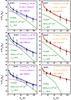 |
Fig. 10 Best-model comparisons between CO observations and models for all positions in W44F (W44F1: top row, W44F2: centre row, W44F3: bottom row) for both the blue (left) and red (right) shock components, respectively. The colour code is the same as in Fig. 9. |
Our grid of models consists of more than 1000 integrated intensity diagrams obtained for C- and CJ-type shock models7. The range of model parameters covered by our grid is listed in Table 5. We note that the coverage of our grid is not completely uniform over the range parameters, therefore the table gives maximum und minimum grid intervals for each parameter as found in our grid. The observed SLEDs were compared with this grid using a χ2 routine to select the best fits. In the fits, we only used the most unambiguous shock-tracing lines CO (7–6) and CO (6–5), which are not expected to be optically thick in the line wings and which are not affected by self-absorption. In W44E, another reason for that choice is the existence of background emission unrelated to W44 in the low-lying CO transitions, which is expected in the velocity range 70–90 km s-1 (see Sect. 4). Because the redshifted line wings stretch much farther in W44E than in W44F, it is impossible to discern this background emission from shocked gas related to W44E. In W44F this problem does not exist because of the narrower line widths, but here the integrated intensities in CO (3–2) and CO (4–3) are only rough estimates based on the line wings and can therefore only serve as additional constraint for the fits based on the higher transitions.
8. Results
8.1. Shock emission
8.1.1. W44E
Our χ2 comparison of the observed integrated intensities of CO in the unambiguously shock tracing transitions (7–6) and (6–5) towards W44E with our grid of models showed the observations to be compatible with non-stationary CJ-shocks. Such shocks have not yet reached a state of dynamical equilibrium. Lesaffre et al. (2004a,b) have proven that such young shocks can be approximated by introducing a J-type discontinuity in a C-type flow at a point in the steady-state profile that is located increasingly downstream as the age of the shock advances, hence their designation as CJ-type. Given their younger shock age, the calculation is subsequently stopped sooner in the post-shock gas. The result is that the overall profile is found to be warmer, but also thinner than that of a stationary C-type shock, resulting in less CO emission, with a characteristic shift of the excitation towards higher-lying transitions. For the blue lobe in W44E2, the integrated line intensities in CO (7–6) and CO (6–5) were found to be consistent with either CJ-type models with a pre-shock density of nH = 104 cm-3, or with C-type ones, with a pre-shock density of 103 cm-3, as can be seen in Fig. 8. Because of the wider and colder thermal profile generated in C-type shocks, it can be seen that the modelled integrated intensities in CO(3–2) and CO(4–3) of a C-type shock strongly overtop the observed ones. For this reason, and because the 103 cm-3 pre-shock density significantly differs from the derived densities in the other positions, we discarded this fitting solution. J-type shocks, on the other hand, do not match our observations because they would predict a higher relative excitation of the higher CO transitions due to the higher temperatures produced in these discontinuous shocks. Based on these considerations, we conclude that young CJ-type shocks seem to be most consistent with our observations. We note that these models are also successful in predicting the optical thickness (thinness) of the lower (upper) lying CO transitions.
Modelling results for W44E: shock emission.
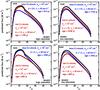 |
Fig. 11 Integrated CO fluxes (W m-2) against the rotational quantum numbers of the upper level in W44E. The highest level of Jup = 40 corresponds to a maximum energy of 4513 K. Displayed are the integrated fluxes for W44E1 as predicted by the high-velocity models (left panel) and low-velocity models (right panel) for W44E1 (top row) and W44E2 (bottom row). |
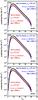 |
Fig. 12 Integrated CO fluxes (W m-2) against the rotational quantum numbers of the upper level in W44F. The highest level of Jup = 40 corresponds to a maximum energy of 4513 K. Displayed are the integrated fluxes for the positions W44F1 (top), W44F2 (middle), and W44F3 (bottom). |
Given the presumably young age of the shocks in the molecular clumps close to the edge of the remnant (being much younger than the assumed SNR’s age of 20 000 years), this result seems reasonable. The pre-shock density is found to be 104 cm-3, consistent with previous estimates for the dense clump component (Reach & Rho 2000; Reach et al. 2005). The total, blue- to redshifted velocity extent of the CO lines towards W44E, which is ~60 km s-1, imposes a constraint on possible shock velocities: the gas must be accelerated to velocities ≥30 km s-1. Obeying this constraint we obtain projected shock velocities of 35 and 30 km s-1 for the blue and the red lobe in W44E1, respectively, while in W44E2 we get 30 and 35 km s-1 for the blue and the red lobe. The pre-shock magnetic field component perpendicular to the shock layers in our models is constrained to B = 200 μG for the blue lobes and 150 or 175 μG for the red lobes in W44E1 and W44E2. The difference could either be attributed to uncertainties in the analysis, be interpreted as a projection effect, or a as a slight inhomogeneity of the medium. The age of the shocks scatters around 1000 years, where the shocks of the dominant lobes for each position (red in W44E1 and blue in W44E2) appear older than the shocks in the reverse directions. In general the whole double-peak structure in W44E bears some bipolar characteristics, where antiparallel shocks exhibit similar parameters, pointing towards a general uniformity of the medium over the observed scales along the line of sight.
We note that the best fits to the observed SLEDs, except for the red lobe in W44E2, were achieved with slow CJ-shocks at ~20 km s-1, which are much less consistent with the broad linewidths. We however also list them (together with the best fit in the 20 km s-1 velocity range towards W44E2, red lobe) in Table 6, as one could argue that they might constitute the dominant shock component as compared to possible faster but weaker components. They agree with the faster solutions in terms of the pre-shock density and the magnetic field strength value, but show higher ages of almost 2000 years.
The post-shock density of all models fitting the observations in W44E is of the order of 9 × 10⁴–1.5 × 105 cm-3, yielding expected post-shock values of the magnetic field for this component of 390–720 μG, compatible with the magnetic field strength estimated from maser circular polarization observations (see Sect. 3.1.1). The models produce OH column densities of a few 1014 cm-2 while the CO column density in the models is of the order of 4 × 10¹⁶–2 × 1017 cm-2.
8.1.2. W44F
The line widths in W44F are narrower than in W44E. Accordingly, we find that the observations are compatible with CJ-type shocks with velocities between 20 km s-1 and 25 km s-1 as best fits to our observations (compare Table 8). The pre-shock magnetic field component perpendicular to the shock layers in our models is given by b =2 corresponding to 200 μG and the pre-shock density given as 104 cm-3, consistent with W44E. The age of the shocks in W44F is ~2900 years. This result is somewhat puzzling given the much younger age obtained for W44E. The difference is less strong if we consider the slow shock solutions in W44E. However, the different line-widths in W44E and F already hint at a different nature of the shocks in both regions, probably linked to inhomogeneities in the ISM. The post-shock density of the models consistent with the CO emission in W44F is of the order of 7 × 10⁴–9 × 104 cm-3, similar to W44E, with corresponding magnetic field values of ~600 μG. The OH column densities are of the order of 7 × 10¹⁴–1 × 1015 cm-2, while for CO the column densities are ~3 × 1017 cm-2.
8.2. Degeneracies of the shock models
To get an idea of the robustness and degeneracy of the results presented in the previous section, we have examined the best-fitting models, having χ2 values of at most twice the smallest value, for each position in both velocity lobes. Except for the two C-type models in W44E2 already mentioned above and some C-type cases in W44F with relatively high values of χ2, all models are CJ-type. Furthermore all these CJ-models agree in a pre-shock value of 104 cm-3.
In W44E, the mean values of the pre-shock magnetic field strengths of the best-fitting models lie within the range of ~150–175 μG with standard deviations of about 40 μG8. The mean velocity values in W44E are located between 22 km s-1 (W44E1, red lobe) and 35 km s-1 (W44E2, red lobe) with a maximum standard deviation of 9 km s-1 (W44E1, blue lobe). The largest scatter among positions and velocity lobes in W44E is found with respect to the ages of the shocks, where the mean values are 1700 and 680 years in W44E2, blue and red lobe respectively, and 1350 and 2000 years in W44E1, blue and red lobe respectively, with standard deviations of ~400 years. However, as will be discussed later, the fitting of the red lobe emission in W44E is subject to increased uncertainties.
In W44F, the best-fitting models lie closer together in terms of their values of χ2 than in W44E. The range of mean values of the pre-shock magnetic field strengths of the best-fitting models in W44F is the same as in W44E with standard deviations of 30–50 μG. The mean velocity values lie between 24 km s-1 and 27 km s-1 with standard deviations of ~5 km s-1. The mean ages of the best-fitting models lie in the range of 2050–2750 years, with standard deviations of the order of 700 years.
8.3. Unshocked CO layers
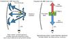 |
Fig. 13 Schematic illustration of our modelling approach. The main SNR shock direction is perpendicular to the line of sight as traced by OH masers, which are known to reside in dense postshock gas. The spectral line broadening, however, hints at supersonic fluid motion along the line of sight, which are expected, given projection effects and complex cloud substructure (left sketch). Our modelling decomposes the complex shock geometry in three components: one shock layer propagating away from the observer (fitting the red-shifted component of the line profiles), one shock layer propagating towards the observer (fitting the blue-shifted emission of the line profiles), and an additional layer of gas (found to correspond to postshock conditions) that extends into the line wings (right sketch). This latter layer makes up for the unrealistic accumulation of matter in the post-shock region inherent to one-dimensional shock modelling, which does not allow the post-shock gas to relax in all possible directions, as well as for existing post-shock gas created and stirred up by shocks perpendicular to the line of sight. |
As already found for W28F (Gusdorf et al. 2012), all fitting shock models underestimate the emission in CO (3–2) and CO (4–3). This is not too surprising as we do not expect our shock models to accurately model the dense and cold postshock gas because of their one-dimensional geometry. Furthermore, the existence of OH masers hints at the presence of dense postshock gas that is due to a shock transverse to the line of sight and thus different from the line-wing shock emission we consider in our shock models (See Fig. 13). We therefore added a layer of CO to the shock models, calculated with the LVG module in homogeneous slab mode. This was done by calculating a large grid with varying density (nH = 104, 5 × 10⁴, and 105 cm-3), temperature (10–150 K), line width (Δν = 1, 5, and 10 km s-1), CO fractional abundance (10-4–10-6), and CO column density (2 ×10¹³–1 × 1020 cm-2). This grid of 2700 models was then compared to the residuals of the shock-modelled integrated intensities in CO (3–2) and CO (4–3) using a χ2 routine. The results are listed in Tables 7 and 9.
Modelling results for W44E: CO layers.
Modelling results for W44F: shock emission.
Modelling results for W44F: CO layers.
Mass, momentum and energy injection per beam for W44E.
Mass, momentum and energy injection per beam for W44F.
In W44E, the layers complementing the shock fits are at low and moderate temperatures between 10 K and 60 K with densities always higher than the obtained preshock density of 104 cm-3. The CO column densities vary between 5 × 1015 cm-2 and 2 × 1019 cm-2. The best-model comparisons of the CO observations and the shock and layer components are displayed in Fig. 9. The sum of both components gives an encouraging fit to the data except for the integrated intensities (or column densities of the upper levels, respectively) of CO (3–2) and (4–3) in the red lobe of the W44E2 position. As we have noted before, the corresponding spectrum extends extremely far in the red-shifted range of the spectrum, showing only weak emission and is therefore prone to possible uncertainties in the baseline subtraction. Given the expected contamination by background emission, a poor baseline quality in CO (4–3), and that our grid of shock models is not well suited for these high shock velocities, it might not be too surprising that our fit was not as successful in this case.
The CO layers complementing the shock models in W44F show temperature values between 30 K and 80 K. The densities, as in W44E, are higher than the obtained preshock density in all added layers. The layer temperatures in the blue wings are always lower than in the red wings. The inferred CO column densities have values between 1016 cm-2 and 2.5 × 1017 cm-2. The quality of the fits, displayed in Fig. 10, is satisfying in all cases. Given their density and temperature values, the added gas layers in W44E and W44F are dominated by postshock gas. We however note that, given the geometric uncertainties, a more detailed interpretation of these layers (e.g. possible contamination by unshocked ambient/foreground gas) has to remain open.
9. Discussion
SNRs consitute an important source of energy and momentum input for the ISM. Tables 10 and 11 show the mass, momentum, and energy injection calculated per beam for our best-fitting shock models. The shocked mass per beam amounts to ~1 and ~2 M⊙ for the models in W44E and F, respectively. The total energy input in one beam, given as the sum of the blue- and the red-lobe shock contributions, amounts to ~1 × 1046 erg in W44E and ~1.5 × 1046 erg in W44F. This contribution approximately corresponds to the fraction of the total initial energy of 1051 erg that is expected to be ejected into the observed area by the supernova, assuming an isotropic explosion. This would mean that the interaction of the SNR with molecular clouds constitutes regions of high energy dissipation. The values of the momentum input as sum of the red- and blue-shifted velocity lobes in one beam lies between ~4 × 10⁶ M⊙ cm s-1 and ~7 × 10⁶ M⊙ cm s-1, while in W44F it is ~1 × 10⁷ M⊙ cm s-1. The results for all positions in both velocity intervals are listed in Tables 10 and 11.
Figures 11 and 12 show the integrated CO fluxes (in W m-2) within our 182
beam for all rotational transitions up to an upper rotational quantum number of 40 for all
best-fitting shock models (compare Hailey-Dunsheath et al.
2012). Displayed are the shock models that fit the red- and blue-wing emission (red
and blue dots, respectively) together with the total line integrated fluxes as sum of both
wings (black dots). The asymmetry of the line profiles in W44E is mirrored in the plots, as
well as the extensive symmetry of the lines in W44F. As can be seen from Fig. 11, observations of higher-lying CO transitions will
provide an opportunity to remove modelling degeneracies, in particular the degeneracy
between slow and fast models in W44E, because the location of the peak in the CO-ladder
differs for different models. Such observations will be possible with the SOFIA telescope.
Given that our fits are based on only two transitions that unambiguously trace shock
emission, it is very important to add more lines to our analysis.
Finally, we must note that the extraction of the integrated intensities relies on some assumptions with respect to the shock geometry in the analysed region. Following the method introduced in the study of Gusdorf et al. (2012), we split the whole spectral line into blue- and red-shifted parts without completely omitting the central line emission. The real situation, however, is most certainly much more complex. The existence of maser spots hints that a dominant shock direction is perpendicular to the line of sight, with the corresponding post-shock emission thus also being found in the line centres. The broad line wings might then stem from the projected wings of a bow-shock, with the ambient medium being compressed and pushed aside (for a schematic illustration see Fig. 13).
Our analysis can only be applied to shock components propagating parallel to the line of sight and therefore gives averaged information on the shock conditions only in the gas being pushed towards or away from us. The derived properties, as long as they are non-directional such as the total magnetic field strength or the density, should still be valid. However, it is important to keep in mind that the geometrical assumptions we applied are severe and a more accurate modelling in terms of geometry would need to account for the influence of the shock component perpendicular to the line of sight as well. At the same time, we note that the high level of microphysical detailedness included in our shock model cannot be maintained within fully two- or three-dimensional models. An alternative would be the use of pseudo-multidimensional models, synthesized from one-dimensional shocks, as presented by e.g. Kristensen et al. (2008) and Gustafsson et al. (2010), but in any case, a multi-dimensional modelling approach would add a set of additional, barely constrained parameters, such as the orientation of the magnetic field with respect to the shock structure, and therefore increase the degeneracy of the modelling in a prohibitive way.
10. Conclusions
-
1.
We have presented new mapping observationswith the APEX telescope in 12CO (3–2),(4–3), (6–5), (7–6), and 13CO (3–2) to-wards regions E and F in W44. The spectra, averagedover the respective regions, exhibit emission featuresat 13 km s-1,corresponding to foreground emission, and emission be-tween 70 km s-1and 90 km s-1,which is at least partly due to background emission(Seta et al. 1998).The averaged lines show broad wing emission, be-tween ~15 km s-1and ~90 km s-1 inW44E and between ~25 km s-1and ~60 km s-1 inW44F. Accordingly the red-shifted emission in W44E is hard todisentangle from background emission.
-
2.
The velocity integrated maps in the blue (20–40 km s-1) and red (50–70 km s-1) velocity regimes in W44E show one red- and one blue- shifted local maximum for all observed transitions, where the red-shifted local maximum (W44E1) is located just behind the forward edge of molecular gas as delineated by OH masers. The blue-shifted local maximum (W44E2) is located farther towards the interior of W44, where maser emission is also observed. In W44F, the thin filament of molecular gas ranging from the north-west to the south-east shows two local maxima in the red-shifted (W44F2 and W44F2) and one in the blue-shifted velocity regime (W44F3), the latter in the very south of the filament, where the red-shifted emission is already very weak.
-
3.
The individual spectra in the W44E1 and W44E2 exhibit two components: one narrow peak of ambient emission at ~45 km s-1, coincident with the emission in 13CO (3–2), and a broad component of shock emission. The shock-broadened lines are asymmetric but bear similar shapes in all 12CO transitions. Towards W44F the lower transitions are subject to strong absorption in their line centres. The lines are narrower and, except for W44F3, also more symmetric than in W44E.
-
4.
The integrated intensities of CO (7–6) and (6–5) of the blue- and red lobe components in these position were compared with a large grid of shock models combined with radiative transfer modules. This comparison revealed non-stationary shock models to be compatible with the observations. These relatively young shocks have ages of no more than 3000 years, consistent with the remnant’s age of 20 000 years. The pre-shock density for all models was found to be 104 cm-3. The best-fitting models in W44E have velocities of ~20 km s-1, which seems low given the broad line widths. We therefore also presented the best-fitting models with velocities ≥30 km s-1. The pre-shock magnetic field strengths of all best-fitting models in W44E are 100–200 μG, while in W44F we found values of 200 μG in all positions.
-
5.
To account for the integrated emission in CO (3–2) and (4–3), CO layers corresponding to post-shock gas had to be added to the shock models. The need for such additional layers stems from the one-dimensional nature of our modelling approach.
-
6.
Based on the best-fitting shock models, we could estimate the shocked gas mass in one beam as well as the momentum- and energy injection per beam. In both regions, the shocked gas masses lie between ~1 M⊙ and 2 M⊙, the momentum injection amounts to 1–5 × 10⁶ M⊙ cm s-1, and the energy injection to 1–8 × 1045 erg in one beam. This energy injection approximately corresponds to the fraction of the total initial energy that is expected to be dissipated in the observed area, assuming an isotropic explosion.
-
7.
Our analysis can only be applied to shock components moving parallel to the line of sight, as revealed by the broad spectral line wings. Our results therefore correspond to mean properties of the shocked gas moving towards and away from us. Furthermore, we stress the present limitation of our analysis with respect to the very small number of unambiguously shock-tracing transitions we used in our fits. In the future, it will be necessary to base the modelling on additional shock-tracing transitions in order to eliminate modelling degeneracies.
Online material
Appendix A: CO Tables
This publication is based on data acquired with the Atacama Pathfinder EXperiment (APEX). APEX is a collaboration between the Max-Planck-Institut für Radioastronomie, the European Southern Observatory, and the Onsala Space Observatory.
This First Light APEX Submillimeter Heterodyne receiver was developed by Max Planck Institut für Radioastronomie, MPIfR, and commissioned in May 2010. In the 345 GHz band the dual-polarization receiver FLASH operates a 2SB SIS mixer provided by IRAM (Maier et al. 2005).
Because Seta et al. (1998) were only able to separate structures larger than ~15 pc, their observations cannot differentiate between W44E and F.
Wootten (1997) notes that there are no molecular absorption features in this velocity regime, therefore he concludes that the emitting gas is situated beyond the remnant.
The grid also contains high-density models subject to grain-grain processing as calculated by Anderl et al. (2013).
A somewhat special case is W44E2, red lobe, where the best fitting, high-velocity model and the second best model have χ2 values that differ by a factor of 2.3, such that there is no considerable fitting degeneracy.
Acknowledgments
We are grateful to an anonymous referee for useful comments that helped to strengthen the paper. We thank Dale Frail for kindly providing us with the radio continuum map at 1442.5 MHz. S. Anderl acknowledges support by the DFG SFB 956, the International Max Planck Research School (IMPRS) for Astronomy and Astrophysics, and the Bonn-Cologne Graduate School of Physics and Astronomy. A. Gusdorf is grateful to Sylvie Cabrit for useful discussions. Moreover, he acknowledges support by the grant ANR-09-BLAN-0231-01 from the French Agence Nationale de la Recherche as part of the SCHISM project.
References
- Abdo, A. A., Ackermann, M., Ajello, M., et al. 2010, Science, 327, 1103 [NASA ADS] [CrossRef] [PubMed] [Google Scholar]
- Ackermann, M., Ajello, M., Allafort, A., et al. 2013, Science, 339, 807 [NASA ADS] [CrossRef] [PubMed] [Google Scholar]
- Anderl, S., Guillet, V., Pineau des Forêts, G., & Flower, D. R. 2013, A&A, 556, A69 [NASA ADS] [CrossRef] [EDP Sciences] [Google Scholar]
- Blandford, R., & Eichler, D. 1987, Phys. Rep., 154, 1 [Google Scholar]
- Blandford, R. D., & Cowie, L. L. 1982, ApJ, 260, 625 [NASA ADS] [CrossRef] [Google Scholar]
- Castelletti, G., Dubner, G., Brogan, C., & Kassim, N. E. 2007, A&A, 471, 537 [NASA ADS] [CrossRef] [EDP Sciences] [Google Scholar]
- Caswell, J. L., Murray, J. D., Roger, R. S., Cole, D. J., & Cooke, D. J. 1975, A&A, 45, 239 [NASA ADS] [Google Scholar]
- Cesarsky, D., Cox, P., Pineau des Forêts, G., et al. 1999, A&A, 348, 945 [NASA ADS] [Google Scholar]
- Chevalier, R. A. 1999, ApJ, 511, 798 [NASA ADS] [CrossRef] [Google Scholar]
- Chieze, J.-P., Pineau des Forets, G., & Flower, D. R. 1998, MNRAS, 295, 672 [NASA ADS] [CrossRef] [Google Scholar]
- Claussen, M. J., Frail, D. A., Goss, W. M., & Gaume, R. A. 1997, ApJ, 489, 143 [NASA ADS] [CrossRef] [Google Scholar]
- Cox, D. P. 2005, ARA&A, 43, 337 [NASA ADS] [CrossRef] [EDP Sciences] [MathSciNet] [Google Scholar]
- Cox, D. P., Shelton, R. L., Maciejewski, W., et al. 1999, ApJ, 524, 179 [NASA ADS] [CrossRef] [Google Scholar]
- Denoyer, L. K. 1983, ApJ, 264, 141 [NASA ADS] [CrossRef] [Google Scholar]
- Dickel, J. R., Dickel, H. R., & Crutcher, R. M. 1976, PASP, 88, 840 [NASA ADS] [CrossRef] [Google Scholar]
- Edge, D. O., Shakeshaft, J. R., McAdam, W. B., Baldwin, J. E., & Archer, S. 1959, Mem. Rev. Astron. Soc., 68, 37 [Google Scholar]
- Elfhag, T., Booth, R. S., Hoeglund, B., Johansson, L. E. B., & Sandqvist, A. 1996, A&AS, 115, 439 [NASA ADS] [Google Scholar]
- Elitzur, M. 1976, ApJ, 203, 124 [NASA ADS] [CrossRef] [Google Scholar]
- Esposito, J. A., Hunter, S. D., Kanbach, G., & Sreekumar, P. 1996, ApJ, 461, 820 [NASA ADS] [CrossRef] [Google Scholar]
- Flower, D. R., & Pineau des Forêts, G. 2003, MNRAS, 343, 390 [NASA ADS] [CrossRef] [Google Scholar]
- Flower, D. R., & Pineau des Forêts, G. 2010, MNRAS, 406, 1745 [NASA ADS] [Google Scholar]
- Flower, D. R., Bourlot, J. L., Pineau des Forêts, G., & Cabrit, S. 2003, MNRAS, 341, 70 [NASA ADS] [CrossRef] [Google Scholar]
- Frail, D. A., & Mitchell, G. F. 1998, ApJ, 508, 690 [NASA ADS] [CrossRef] [Google Scholar]
- Frail, D. A., Giacani, E. B., Goss, W. M., & Dubner, G. 1996, ApJ, 464, L165 [NASA ADS] [CrossRef] [Google Scholar]
- Giacani, E. B., Dubner, G. M., Kassim, N. E., et al. 1997, AJ, 113, 1379 [NASA ADS] [CrossRef] [Google Scholar]
- Giannini, T., McCoey, C., Caratti o Garatti, A., et al. 2004, A&A, 419, 999 [NASA ADS] [CrossRef] [EDP Sciences] [Google Scholar]
- Giuliani, A., Cardillo, M., Tavani, M., et al. 2011, ApJ, 742, L30 [NASA ADS] [CrossRef] [Google Scholar]
- Green, D. A. 1989, MNRAS, 238, 737 [NASA ADS] [CrossRef] [Google Scholar]
- Gusdorf, A., Pineau des Forêts, G., Cabrit, S., & Flower, D. R. 2008, A&A, 490, 695 [NASA ADS] [CrossRef] [EDP Sciences] [Google Scholar]
- Gusdorf, A., Giannini, T., Flower, D. R., et al. 2011, A&A, 532, A53 [Google Scholar]
- Gusdorf, A., Anderl, S., Güsten, R., et al. 2012, A&A, 542, L19 [NASA ADS] [CrossRef] [EDP Sciences] [Google Scholar]
- Gustafsson, M., Ravkilde, T., Kristensen, L. E., et al. 2010, A&A, 513, A5 [NASA ADS] [CrossRef] [EDP Sciences] [Google Scholar]
- Güsten, R., Nyman, L. Å., Schilke, P., et al. 2006, A&A, 454, L13 [NASA ADS] [CrossRef] [EDP Sciences] [Google Scholar]
- Güsten, R., Baryshev, A., Bell, A., et al. 2008, in SPIE Conf. Ser., 7020, 10 [Google Scholar]
- Hailey-Dunsheath, S., Sturm, E., Fischer, J., et al. 2012, ApJ, 755, 57 [NASA ADS] [CrossRef] [Google Scholar]
- Harrus, I. M., Hughes, J. P., & Helfand, D. J. 1996, ApJ, 464, L161 [NASA ADS] [CrossRef] [Google Scholar]
- Heyminck, S., Kasemann, C., Güsten, R., de Lange, G., & Graf, U. U. 2006, A&A, 454, L21 [NASA ADS] [CrossRef] [EDP Sciences] [Google Scholar]
- Hoffman, I. M., Goss, W. M., Brogan, C. L., & Claussen, M. J. 2005, ApJ, 627, 803 [NASA ADS] [CrossRef] [Google Scholar]
- Jones, L. R., Smith, A., & Angelini, L. 1993, MNRAS, 265, 631 [NASA ADS] [CrossRef] [Google Scholar]
- Kasemann, C., Güsten, R., Heyminck, S., et al. 2006, in SPIE Conf. Ser., 6275 [Google Scholar]
- Kawasaki, M., Ozaki, M., Nagase, F., Inoue, H., & Petre, R. 2005, ApJ, 631, 935 [NASA ADS] [CrossRef] [Google Scholar]
- Klein, B., Philipp, S. D., Krämer, I., et al. 2006, A&A, 454, L29 [NASA ADS] [CrossRef] [EDP Sciences] [Google Scholar]
- Klein, B., Hochgürtel, S., Krämer, I., et al. 2012, A&A, 542, L3 [NASA ADS] [CrossRef] [EDP Sciences] [Google Scholar]
- Knapp, G. R., & Kerr, F. J. 1974, A&A, 33, 463 [NASA ADS] [Google Scholar]
- Koo, B.-C., & Heiles, C. 1995, ApJ, 442, 679 [NASA ADS] [CrossRef] [Google Scholar]
- Kristensen, L. E., Ravkilde, T. L., Pineau des Forêts, G., et al. 2008, A&A, 477, 203 [NASA ADS] [CrossRef] [EDP Sciences] [Google Scholar]
- Kundu, M. R., & Velusamy, T. 1972, A&A, 20, 237 [NASA ADS] [Google Scholar]
- Langer, W. D., & Penzias, A. A. 1993, ApJ, 408, 539 [NASA ADS] [CrossRef] [Google Scholar]
- Lesaffre, P., Chièze, J.-P., Cabrit, S., & Pineau des Forêts, G. 2004a, A&A, 427, 147 [NASA ADS] [CrossRef] [EDP Sciences] [Google Scholar]
- Lesaffre, P., Chièze, J.-P., Cabrit, S., & Pineau des Forêts, G. 2004b, A&A, 427, 157 [NASA ADS] [CrossRef] [EDP Sciences] [Google Scholar]
- Lockett, P., Gauthier, E., & Elitzur, M. 1999, ApJ, 511, 235 [NASA ADS] [CrossRef] [Google Scholar]
- Maciejewski, W., Murphy, E. M., Lockman, F. J., & Savage, B. D. 1996, ApJ, 469, 238 [NASA ADS] [CrossRef] [Google Scholar]
- McKee, C. F., & Cowie, L. L. 1975, ApJ, 195, 715 [NASA ADS] [CrossRef] [Google Scholar]
- McKee, C. F., & Cowie, L. L. 1977, ApJ, 215, 213 [NASA ADS] [CrossRef] [Google Scholar]
- Meijerink, R., Kristensen, L. E., Weiß, A., et al. 2013, ApJ, 762, L16 [NASA ADS] [CrossRef] [Google Scholar]
- Mills, B. Y., Slee, O. B., & Hill, E. R. 1958, Austr. J. Phys., 11, 360 [NASA ADS] [CrossRef] [Google Scholar]
- Muders, D., Hafok, H., Wyrowski, F., et al. 2006, A&A, 454, L25 [NASA ADS] [CrossRef] [EDP Sciences] [Google Scholar]
- Neufeld, D. A., Hollenbach, D. J., Kaufman, M. J., et al. 2007, ApJ, 664, 890 [NASA ADS] [CrossRef] [MathSciNet] [Google Scholar]
- Paron, S., Ortega, M. E., Rubio, M., & Dubner, G. 2009, A&A, 498, 445 [NASA ADS] [CrossRef] [EDP Sciences] [Google Scholar]
- Petre, R., Kuntz, K. D., & Shelton, R. L. 2002, ApJ, 579, 404 [NASA ADS] [CrossRef] [Google Scholar]
- Radhakrishnan, V., Goss, W. M., Murray, J. D., & Brooks, J. W. 1972, ApJS, 24, 49 [NASA ADS] [CrossRef] [Google Scholar]
- Reach, W. T., & Rho, J. 1996, A&A, 315, L277 [NASA ADS] [Google Scholar]
- Reach, W. T., & Rho, J. 1998, ApJ, 507, L93 [NASA ADS] [CrossRef] [Google Scholar]
- Reach, W. T., & Rho, J. 2000, ApJ, 544, 843 [NASA ADS] [CrossRef] [Google Scholar]
- Reach, W. T., Rho, J., & Jarrett, T. H. 2005, ApJ, 618, 297 [NASA ADS] [CrossRef] [Google Scholar]
- Rho, J., & Petre, R. 1998, ApJ, 503, L167 [NASA ADS] [CrossRef] [Google Scholar]
- Rho, J., Petre, R., Schlegel, E. M., & Hester, J. J. 1994, ApJ, 430, 757 [NASA ADS] [CrossRef] [Google Scholar]
- Scheuer, P. A. G. 1963, The Observatory, 83, 56 [NASA ADS] [Google Scholar]
- Scoville, N. Z., Yun, M. S., Sanders, D. B., Clemens, D. P., & Waller, W. H. 1987, ApJS, 63, 821 [NASA ADS] [CrossRef] [Google Scholar]
- Seta, M., Hasegawa, T., Dame, T. M., et al. 1998, ApJ, 505, 286 [NASA ADS] [CrossRef] [Google Scholar]
- Seta, M., Hasegawa, T., Sakamoto, S., et al. 2004, AJ, 127, 1098 [NASA ADS] [CrossRef] [Google Scholar]
- Shelton, R. L., Cox, D. P., Maciejewski, W., et al. 1999, ApJ, 524, 192 [NASA ADS] [CrossRef] [Google Scholar]
- Smith, A., Jones, L. R., Watson, M. G., et al. 1985, MNRAS, 217, 99 [NASA ADS] [CrossRef] [Google Scholar]
- Szymkowiak, A. E. 1980, in Type I supernovae, Proc. of the Texas Workshop, 32 [Google Scholar]
- Taylor, J. H., & Cordes, J. M. 1993, ApJ, 411, 674 [NASA ADS] [CrossRef] [Google Scholar]
- Velusamy, T. 1988, in IAU Colloq. 101, Supernova Remnants and the Interstellar Medium, eds. R. S. Roger, & T. L. Landecker, 265 [Google Scholar]
- Watson, M. G., Willingale, R., Pye, J. P., et al. 1983, in Supernova remnants and their X-ray emission, Proc. of the Symp., 101, 273 [NASA ADS] [Google Scholar]
- Westerhout, G. 1958, Bulletin of the Astronomical Institutes of the Netherlands, 14, 215 [Google Scholar]
- White, R. L., & Long, K. S. 1991, ApJ, 373, 543 [NASA ADS] [CrossRef] [Google Scholar]
- ,Wolszczan Cordes, J. M., & Dewey, R. J. 1991, ApJ, 372, L99 [NASA ADS] [CrossRef] [Google Scholar]
- Woltjer, L. 1972, ARA&A, 10, 129 [NASA ADS] [CrossRef] [Google Scholar]
- Wootten, H. A. 1977, ApJ, 216, 440 [NASA ADS] [CrossRef] [Google Scholar]
- Yuan, Y., & Neufeld, D. A. 2011, ApJ, 726, 76 [NASA ADS] [CrossRef] [Google Scholar]
All Tables
Observed lines, and associated frequencies, beam sizes, sampling, and forward efficiencies.
All Figures
|
Fig. 1 Location of the fields covered by our CO observations on the larger-scale radio continuum image at 1442.5 MHz, taken from Giacani et al. (1997). The wedges indicate the intensity of the continuum in Jy/beam. Left panel: entire SNR, right panel: zoom in the regions W44E and W44F. The inserts show the distribution of the CO (6–5) emission, integrated between 20 km s-1 and 70 km s-1, for which the colourscale is in the range 0–50 K km s-1, and the contours are radio continuum in steps of 10 mJy. The size of the zoombox is ~10.3 × 12.4 pc. |
| In the text | |
|
Fig. 2 CO spectra (in TMB) averaged over the W44E (top) and W44F (bottom) regions. The spectra correspond to the transitions of CO (3–2) (black), CO (4–3) (pink), CO (6–5) (blue), and CO (7–6) (light blue). The CO spectral resolutions are 2.18 km s-1 for CO (7–6) in W44F, and 1.0 km s-1 for all other lines. |
| In the text | |
|
Fig. 3 Overlays of the velocity-integrated maps of CO (3–2) (left
column), CO (4–3) (middle column), and CO (7–6)
(right column) as white contours on the CO (6–5) emission (colour
background) observed towards W44E with the APEX telescope. The maps are in their
original resolution (9 |
| In the text | |
|
Fig. 4 Same as Fig. 3 but observed towards W44F. The black and blue hexagons mark the positions of the OH masers observed by Claussen et al. (1997) and Hoffman et al. (2005). |
| In the text | |
|
Fig. 5 Central Panel: positions of our analysis in W44E (W44E1: black
circle, W44E2: blue circle) on the velocity-integrated CO (6–5) emission
( |
| In the text | |
|
Fig. 6 Same as Fig. 5 but towards W44F. The positions in the central panel are W44F1, W44F2, and W44F3 (north to south). Left panel: spectra observed in the position W44F3. Right panel: spectra observed in the position W44F1 (top) and W44F2 (bottom). The CO spectral resolutions are 2.18 km s-1 for CO (7–6) and 1.0 km s-1 for all other lines. |
| In the text | |
|
Fig. 7 Spectra (in TMB) of 12CO (3–2) (grey, left ordinate) and 13CO (3–2) (green, left ordinate) together with the line temperature ratio of 12CO (3–2)/13CO (3–2) (dots, right ordinate). The ratio is shown for 13CO (3–2) line temperatures higher than 2σ (orange dots) and 3σ (red dots). Grey dotted lines indicate values of the temperature ratio as displayed on the left-hand side of these lines. The positions displayed are W44E1 and W44E2, and W44F1, W44F2, and W44F3 (top to bottom). The corresponding values of the optical thickness in the line wings are in the range of 3–7. |
| In the text | |
|
Fig. 8 Rotational diagram of the blue shock component in W44E2. Observations are marked by black squares. The lines show the C-type (dark blue) and CJ-type (light blue) shocks that yield the best fits to the CO (7–6) and (6–5) transitions. |
| In the text | |
|
Fig. 9 Best-model comparisons between CO observations and models for all positions in W44E (W44E1: top row, W44E2: bottom row) for both the blue and red shock components, respectively. The four panels on the left show the high velocity fits while the four panels on the right show the low velocity fits in each position. Observations are marked by black squares, the best-shock models are displayed in violet line (blue lobe) and orange line (red lobe) and diamonds, the CO layer that we used to compensate the ambient emission affecting the CO (3–2) and CO (4–3) transitions in green line and triangels, and the sum of ambient and shock component in blue line (blue lobe) and red line (red lobe) with circles. |
| In the text | |
|
Fig. 10 Best-model comparisons between CO observations and models for all positions in W44F (W44F1: top row, W44F2: centre row, W44F3: bottom row) for both the blue (left) and red (right) shock components, respectively. The colour code is the same as in Fig. 9. |
| In the text | |
|
Fig. 11 Integrated CO fluxes (W m-2) against the rotational quantum numbers of the upper level in W44E. The highest level of Jup = 40 corresponds to a maximum energy of 4513 K. Displayed are the integrated fluxes for W44E1 as predicted by the high-velocity models (left panel) and low-velocity models (right panel) for W44E1 (top row) and W44E2 (bottom row). |
| In the text | |
|
Fig. 12 Integrated CO fluxes (W m-2) against the rotational quantum numbers of the upper level in W44F. The highest level of Jup = 40 corresponds to a maximum energy of 4513 K. Displayed are the integrated fluxes for the positions W44F1 (top), W44F2 (middle), and W44F3 (bottom). |
| In the text | |
|
Fig. 13 Schematic illustration of our modelling approach. The main SNR shock direction is perpendicular to the line of sight as traced by OH masers, which are known to reside in dense postshock gas. The spectral line broadening, however, hints at supersonic fluid motion along the line of sight, which are expected, given projection effects and complex cloud substructure (left sketch). Our modelling decomposes the complex shock geometry in three components: one shock layer propagating away from the observer (fitting the red-shifted component of the line profiles), one shock layer propagating towards the observer (fitting the blue-shifted emission of the line profiles), and an additional layer of gas (found to correspond to postshock conditions) that extends into the line wings (right sketch). This latter layer makes up for the unrealistic accumulation of matter in the post-shock region inherent to one-dimensional shock modelling, which does not allow the post-shock gas to relax in all possible directions, as well as for existing post-shock gas created and stirred up by shocks perpendicular to the line of sight. |
| In the text | |
Current usage metrics show cumulative count of Article Views (full-text article views including HTML views, PDF and ePub downloads, according to the available data) and Abstracts Views on Vision4Press platform.
Data correspond to usage on the plateform after 2015. The current usage metrics is available 48-96 hours after online publication and is updated daily on week days.
Initial download of the metrics may take a while.