| Issue |
A&A
Volume 568, August 2014
|
|
|---|---|---|
| Article Number | A10 | |
| Number of page(s) | 8 | |
| Section | Astronomical instrumentation | |
| DOI | https://doi.org/10.1051/0004-6361/201323326 | |
| Published online | 06 August 2014 | |
Impact on asteroseismic analyses of regular gaps in Kepler data
1 Laboratoire AIM, CEA/DSM – CNRS – Univ. Paris Diderot – IRFU/SAp, Centre de Saclay, 91191 Gif-sur-Yvette Cedex, France
e-mail: This email address is being protected from spambots. You need JavaScript enabled to view it.
2 Space Science Institute, 4750 Walnut Street, Suite 205, Boulder, Colorado 80301, USA
3 Instituto de Astrofísica de Canarias, 38200 La Laguna, Tenerife, Spain
4 Departamento de Astrofísica, Universidad de La Laguna, 38206 La Laguna, Tenerife, Spain
5 Sydney Institute for Astronomy, School of Physics, University of Sydney, NSW 2006, Australia
6 Université de Toulouse, UPS-OMP, IRAP, 31400 Toulouse, France
7 CNRS, Institut de Recherche en Astrophysique et Planétologie, 14 avenue Édouard Belin, 31400 Toulouse, France
8 Instituut voor Sterrenkunde, Katholieke Universiteit Leuven, Celestijnenlaan 200D, 3001 Leuven, Belgium
Received: 23 December 2013
Accepted: 21 May 2014
Abstract
Context. The NASA Kepler mission has observed more than 190 000 stars in the constellations of Cygnus and Lyra. Around 4 years of almost continuous ultra high-precision photometry have been obtained reaching a duty cycle higher than 90% for many of these stars. However, almost regular gaps due to nominal operations are present in the light curves on different time scales.
Aims. In this paper we want to highlight the impact of those regular gaps in asteroseismic analyses, and we try to find a method that minimizes their effect on the frequency domain.
Methods. To do so, we isolate the two main time scales of quasi regular gaps in the data. We then interpolate the gaps and compare the power density spectra of four different stars: two red giants at different stages of their evolution, a young F-type star, and a classical pulsator in the instability strip.
Results. The spectra obtained after filling the gaps in the selected solar-like stars show a net reduction in the overall background level, as well as a change in the background parameters. The inferred convective properties could change as much as ~200% in the selected example, introducing a bias in the p-mode frequency of maximum power. When asteroseismic scaling relations are used, this bias can lead to a variation in the surface gravity of 0.05 dex. Finally, the oscillation spectrum in the classical pulsator is cleaner than the original one.
Key words: asteroseismology / methods: data analysis / stars: oscillations
© ESO, 2014
1. Introduction
Since its launch until the end of the nominal mission (2009−2013), Kepler (Borucki et al. 2010) collected light curves for almost 200 000 stars with varied observation lengths ranging from one month to almost four years (e.g. Huber et al. 2014). The telescope pointed towards the Cygnus & Lyra constellations with a 115 deg2 field of view. The mission has already accomplished many breakthroughs in extrasolar planet research (e.g. Holman et al. 2010; Batalha et al. 2011; Borucki et al. 2012; Carter et al. 2012; Borucki et al. 2013; Huber et al. 2013). In addition, it is contributing strongly to stellar physics through asteroseismology. The long and quasi-continuous light curves of several years have made it possible to probe the overall properties of thousands of solar-like stars and red giants (Chaplin et al. 2011, 2014; Basu et al. 2011; Mosser et al. 2012a; Stello et al. 2013), as well as their internal structure (e.g. Bedding et al. 2011; Mathur et al. 2012; Gruberbauer et al. 2013) and their internal rotation (Beck et al. 2012; Mosser et al. 2012b; Deheuvels et al. 2012).
The Earth-trailing orbit of the mission helped to maximize the observing time while optimizing the duty cycle (in many cases above 90%). During its nominal mission, Kepler underwent several operations that affect the scientific data acquisition and produce almost regular gaps in the light curves. Although these gaps have little impact on the exoplanet search in the time domain, they can have a significant impact on seismic studies based on the frequency domain.
There were three main operations causing quasi-regular gaps in the Kepler scientific data acquisition. The first was the angular momentum dump (AMD), in which the reaction wheels – used for attitude control of the satellite – were desaturated. In general, they occurred about every three days and produced typical gaps of one long-cadence (29.42 min) or several short-cadence (58.85 s) measurements (for more details see the Kepler Data Characteristics Handbook, Christiansen et al. 2013, hereafter KDCH). The second cause was the downlink Earth pointing (DEP). At the end of every “Kepler month” (30.12 days, on average), the spacecraft stopped observing for ~0.9 days to send the data stored in the satellite to the ground station (see Fig. 1). Finally, a third regular operation was performed four times per year – once every quarter (Q) – when the satellite was rolled by 90° about its axis to keep the solar panels illuminated and the radiators away from the Sun. This operation generally took place during the standard DEP, and no additional time was required. However, three gaps were longer than the median value of the data interruptions (see Fig. 1). They were the gaps between Q1 and Q2, Q7 and Q8, and between the first and second months of Q16.
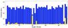 |
Fig. 1 Duration of observations (blue bars) and data gaps (yellow bars) during the 47 “Kepler months”, from Q0 to Q16. The Kepler scientific observations started on May 2, 2009 at 00:55 UT time. |
In addition to these regular events, there were other irregular instrumental problems producing small interruptions in the scientific operations, including the reaction wheels crossing zero angular momentum, losses of spacecraft fine pointing, and sudden pixel sensitivity drop-outs. These caused occasional outliers visible in the Kepler simple-aperture-photometry light curves (usually called the raw data series). Owing to the random nature of these events, the impact on the frequency spectrum was less noticeable than the aforementioned semi-regular events.
The main consequences of the regular gaps are to modify the background power in the Fourier domain and to introduce sequences of harmonics at high frequency. It is therefore important to properly address this potential problem because it can bias the estimations of the parameters of the convective background and the value of νmax, i.e. the frequency of the maximum power of the acoustic modes (e.g. Huber et al. 2009; Mathur et al. 2010b). The latter parameter is used to infer the general properties of stars, such as their masses and radii (e.g. Stello et al. 2008; Chaplin et al. 2011; Mathur et al. 2011; Belkacem et al. 2011; Chaplin et al. 2014).
In this paper we start in Sect. 2 by studying the impact of the quasi-regular gaps in the Kepler spectral window. In Sect. 3, we present a method to minimize the effects of such regular gaps and show some results that concern analysis of the convective background of a young F-type stars, the study of two evolved red giants at different stages of their evolution, and a typical classical pulsator in the instability strip.
2. Impact of the Kepler window function
To characterize the impact of the interruption on the data acquisition from the AMD and the DEP, we decomposed the observed signal, Y(t) as the ideal continuous signal, X(t), multiplied by the window function, W(t):  (1)where the window function, W(t), includes the two main Kepler interruptions. In the case of long-cadence observations,
- 1.
AMD gaps can be modeled by a Dirac Comb function:
 (2)where T1 is three days (see the spectral response in the top panel of Fig. 2);
 - 2.
The gaps due to the DEP can be modelled by a rectangular window convolved with a Dirac comb function:
 (3)where
  is 0.9 days and T2 is one Kepler month (see the spectral response in the bottom panel of Fig. 2).
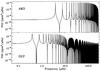 |
Fig. 2 Spectral windows of the gaps induced by the angular momentum dump (AMD, top) and the downlink Earth pointing (DEP, bottom), respectively. |
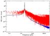 |
Fig. 3 Power spectral density (PSD) on logarithmic scale of a 2 μHz ideal sine wave (black) following the Barycentric Kepler Julian Date (BKJD, see Appendix A for further details). The red curve corresponds to the PSD of the same sine wave multiplied by the Kepler window function. Both PSDs were computed using a Lomb-Scargle algorithm. The blue line is the PSD resulting from converting the timing BKJD of the ideal sine wave (without gaps) into a regular grid and computed using a FFT. |
An example of the power spectral density (PSD) of a sine wave of 2 μHz frequency, computed using a Lomb-Scargle algorithm (Scargle 1982), is shown in Fig. 3. This sine wave has been simulated using the barycentric Kepler Julian date (BKJD) corresponding to the long-cadence measurements of KIC 3733735 in the ideal case (without gaps). A detailed discussion of the Kepler timing can be found in Appendix A. The red curve in Fig. 3 corresponds to the PSD of the same simulation after we have multiplied the ideal observations by the Kepler window function (i.e. adding the observational gaps). As expected, at high frequency (above ~10 μHz), the spectrum is dominated by the three-day harmonics due to the AMD gaps. The increase in the level of power is about five orders of magnitude close to the Nyquist frequency. At lower frequencies down to the central frequency of the sine wave, the spectrum shows an increase in the power compared to the ideal case without gaps, following the trends induced by the DEP gaps.
3. Interpolating the gaps in Kepler observations
To minimize the impact of the regular gaps in the Kepler light curves, we propose to properly interpolate the time series. In the case of the AMD gaps, and because they are small (typically 1 long-cadence point every 3 days), the interpolation can be done with any simple interpolation algorithm. To illustrate that, we compare the PSD of a typical red giant observed in long cadence by Kepler before and after interpolating the data. The Q0-Q16SAP (simple aperture photometry, Christiansen et al. 2013) light curve of this star, KIC 2305930, has been corrected for instrumental perturbations, and the quarters were stitched together following the procedures described by García et al. (2011). The final light curve was high-pass filtered using a triangular smooth function of a 100-day width. The PSD is dominated at high frequency by the harmonics of the AMD gaps (see Fig.4).
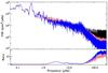 |
Fig. 4 Top: PSD on logarithmic scale of KIC 2305930 smoothed using a 3-point boxcar function. The black curve corresponds to the original light curve. The pink curve is the PSD after correcting all the gaps with sizes less than 1 h (two long-cadence points), while the blue curve is the PSD after inpainting all the gaps less than 20 days. Bottom: ratio between the interpolated PSDs and the one with all the gaps. Both curves have been smoothed using a 300 point boxcar function. |
It is important to note that the original NASA’s pre-search data conditioning pipeline (PDC) – utilized to correct the Kepler light curves (Jenkins et al. 2010) – high-pass filters the data such that periods longer than three days are slightly affected, while periods longer than 20 days are almost entirely removed (see Fig. 1 in Thompson et al. 2013). An improved version of this pipeline called PDC-MAP or PDC-msMAP – where msMAP stands for multi-scale Maximum A Posteriori – used a Bayesian approach to keep part of the low frequency signal. However, in some quarters the algorithm cannot distinguish between instrumental noise and stellar variability, and the signal is completely removed for periods above ~21 days. (García et al. For a comparison of the different corrections methods see 2013.)
We then interpolated all the gaps in the light curve of KIC 2305930 with lengths equal to or smaller than one hour (hence only AMD gaps) using a third-order polynomial fit around the gaps (Ballot et al. 2011). The resulting PSD is shown in Fig. 4. As expected, only the high-frequency harmonics of the AMD gaps are removed, and the rest of the spectrum stays the same (see bottom panel of Fig. 4). It is important to notice that the harmonics of the AMD gaps are only visible in the PSD if the star has periodic signals (e.g. surface rotation signatures or low-frequency pulsations) with periods longer than three days.
To go further, we need to interpolate the ~0.9 day gaps between the “Kepler months” due to the DEP – as well as the three longer ones – in order to remove the spurious trends introduced by the missing data. For this purpose, it is necessary to use an interpolation algorithm that is able to deal with a wide range of gap sizes while preserving the main oscillatory signal and the background as much as possible.
Several methods have been proposed to interpolate seismic data (e.g. Fahlman & Ulrych 1982; Brown & Christensen-Dalsgaard 1990). Although they work quite well, they require an a priori knowledge of the signal to be treated. Therefore, these techniques are not suited to treating thousands of unknown asteroseismic targets. We propose to use an inpainting technique (Elad et al. 2005) based on a prior of sparsity instead. This method assumes that there is a representation of the signal in which most of the coefficients are close to zero. For example, if the signal was a single sine wave, the sparsest representation would be the Fourier transform because most of the Fourier coefficients would be zero except one (hence sparse), which is sufficient to represent the sine wave in the frequency space. Therefore in asteroseismology, and to deal with the large variation in gap sizes (from 1 short-cadence data point to ~16 days), the best representation is a multi-scale discrete cosine transform (MDCT, Starck & Murtagh 2006). Inpainting techniques have already been used several times in astrophysics (e.g. Abrial et al. 2008; Pires et al. 2009), as well as in asteroseismology to correct a few solar-like stars (e.g. Mathur et al. 2010a, 2013; Sato et al. 2010; Ballot et al. 2011) observed by the CoRoT satellite (Baglin et al. 2006). An example of the inpainted light curve of KIC 3733735 can be seen in Fig. 5 for quarters Q7 and Q8.
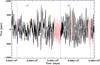 |
Fig. 5 Long cadence light curve of KIC 3733735 (black) for quarters Q7 and Q8. The limit of the quarters are indicated by vertical blue dotted lines. The red line corresponds to the inpainted segments. |
This inpainting algorithm has the additional advantage of being very fast compared to other techniques, such as the CLEAN periodogram (Roberts et al. 1987; Foster 1995). It requires less than a minute for a Q0-Q16 long cadence light curve (see Pires et al. 2014 for a more complete description of the algorithm and its application to asteroseismic data1) when it is applied to regularly sampled data. In the case of Kepler, we need to convert the BKJD irregular time series into a regular grid of points. To do so we use the nearest neighbor resampling algorithm (Broersen 2009). We therefore built a new time series with a sampling rate equal to the median of the original. Each point of the new series is built from the closest observation (irregularly sampled) if it is within half of the new sampling distance. The regular grid point is left empty (nought) if there is no original observation falling within the new sampling. An example of this methodology is shown in Fig. 3. The increase in noise is only visible above ~50 μHz, and it is negligible compared to the noise introduced by the window function (see Appendix B for further details).
Therefore, we propose to inpaint all the gaps in the Kepler time series – with sizes smaller than 20 days – into a regular grid of points with a sampling rate equal to the median sampling rate of each star. By doing so, the Nyquist frequency is fixed to the value determined by the regular sampling rate, and we lose the possibility of exploring frequency regimes above the formal Nyquist frequency, as recently done by Murphy et al. (2013) and Beck et al. (2013). Finally, gaps longer than 20 days – including missing quarters – are too long to be treated in this way. The inpainting algorithm needs to be tested further in these conditions, but this is beyond the scope of this paper.
The resulting power spectrum of the inpainted time series for KIC 2305930 is shown in Fig. 4 (hearafter all the PSDs plotted in blue are computed using inpainted time series). In this case, we see not only an improvement at high frequency, but also at intermediate frequencies, between 1.5 and 10 μHz. Indeed the background level is reduced by a factor of ~2.5 in this region, while the ratio was flat when only AMD gaps were interpolated (see bottom panel of Fig. 4). In the region dominated by the p modes (10−40 μHz), the PSD is the same (ratio of 1), and there is no significant improvement when we interpolate the DEP gaps.
Because the effect of the Kepler window function depends on the characteristics of the stellar signal, we also show the result of inpainting all the gaps in three other stars: KIC 8905990, an evolved M giant (e.g. Bányai et al. 2013; Mosser et al. 2013) with νmax ~ 0.4 μHz observed in long cadence for the full mission; KIC 3733735, a young F-type star (νmax ~ 2130 μHz) continuously observed in short cadence since Q5 (see e.g. Appourchaux et al. 2012; Mathur et al. 2014); and KIC 5892969, a classical pulsator in the instability strip.
In the case of the evolved red giant KIC 8905990, the PSD of the long-cadence Q0−Q16 light curve corrected following García et al. (2011) is shown before and after inpainting the gaps in Fig. 6. The improvement in the background at frequencies above 2 μHz is greater than in the previous case. The shape of the background was completely dominated by the spectral window (black curve) and after interpolating the gaps (blue curve), we reach a reduction in the noise level of three orders of magnitude at high frequency (see bottom panel of Fig. 6).
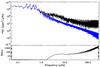 |
Fig. 6 As in Fig. 4, but for the evolved red giant KIC 8905990. In black the PSD for the original Kepler time series, while in blue is the inpainted one. Bottom panel: ratio between both PSDs. |
For the young F star KIC 3733735 observed in short cadence, we used the Q5-Q16 PDC-msMAP (Pre-search Data Conditioning-multi scale Maximum A Posteriori, Christiansen et al. 2013) corrected data to show that the interpolation works well with any type of corrected light curves. The improvement in the inpainted PSD is located at high frequencies compared to the previous stars (see Fig. 7). We achieve a reduction in the background of a factor of 1.6 between ~50 and 400 μHz. This region is dominated by the convective background, and the reduction in the noise has a non negligible impact on the convection properties we can infer.
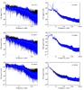 |
Fig. 8 Results of the background fits as describe in the text for three red giants (left panels) and three solar-like stars smoothed over 10 bins (right panels). Spectra obtained from gapped data are shown in black, while spectra after inpainting the light curves are in blue. The background fits are represented in red (resp. green) for the data with gaps (resp. inpainted data). |
To quantify the change on the convective parameters, we analysed a sample of red giants and main-sequence stars. We followed a similar methodology to the one described by Mathur et al. (2011). We fitted a constant photon noise component dominating the spectrum at high frequency, two Harvey-like functions (Harvey 1985) to measure the granulation contribution, and a power law to take the magnetic and rotation signatures at low frequency into account. For the red giants and the solar-like stars, we fixed the slopes of the Harvey-like functions to four (as suggested by Kallinger et al. 2014).
To help quantify the changes, Table 1 provides the background parameters and their statistical uncertainties before and after interpolating the light curves. For red giants, the white noise changes drastically with an average decrease of 90% when the light curves are inpainted. For the granulation time scale and amplitude, there is no systematic decrease or increase, but by inpainting the data they vary between 10% and 40% for τgran and 20% to 200% for Agran. For the solar-like stars, we observe a decrease in the white noise between 2% and 18%, a positive or negative change in τgran between 1% and 90%, and a decrease in Agran from 2% to 35%. Compared to the formal uncertainties provided on these parameters, the changes are significant.
Table 1 also lists the frequency of maximum power of the acoustic modes, νmax, determined by fitting a Gaussian to the p-mode envelope. We notice that for some cases, there is a non-negligible change in the estimated value. This can potentially introduce a bias in the inferred stellar gravity if one uses the νmax vs. log g proportionality. For the sample of stars presented here, this can lead up to a 0.05 dex variation, i.e. 10σ.
Background parameters of six red giants and eight solar-like stars (separated by a horizontal line) for the two types of datasets (with gaps “std” and the inpainted data “inp”).
Finally, in Fig. 9 we show the PSD of the original (black) and inpainted (blue) light curves for the classical pulsator in the instability strip KIC 5892969. In this case, the ratio of the two spectra reveals that in the regions between the main modes, the background signal (or the “grass level”) has been reduced by a factor of 5 to 7.
This is confirmed when we zoom into the region between the modes. An example is shown in Fig. 10. The increase in the signal-to-noise ratio is clear. Most of the “grass” of peaks have disappeared as a consequence of the reduction in the spectral window. Some new modes seem to rise. However, a detailed analysis of the nature of these peaks is beyond the scope of this paper.
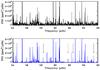 |
Fig. 10 Zoom of the PSD shown in Fig.9 for a region of the PSD between 54 and 66 μHz. The top panel corresponds to the original PSD, and the bottom panel is the PSD obtained from the inpainted light curve (in blue). Vertical arrows mark new peaks found with this analysis. |
4. Conclusions
In this paper we have studied the nature of the regular gaps due to the nominal operations of the NASA Kepler mission. The first sort of gaps are due to the angular momentum desaturation of the reaction wheels, which produce an interruption of the data acquisition of one long-cadence point every three days. These gaps produce a series of harmonics at multiples of three days (3.86 μHz). To avoid this, and because the size of the gaps is so small, simple interpolation algorithms can be used to interpolate the missing data. The resulting interpolated PSD removes any signatures of these harmonics.
The second type of regular gaps is due to the monthly data downlink to Earth. These gaps have a size around 0.9 day on average and thus, it is necessary to use a more complex interpolation algorithm. The effect of these gaps is more subtle and produce a trend in the background at all frequencies.
The light curves interpolated with a third-order polynomial fitting or inpainting show a lower background level in the four categories of stars analysed: two red giants at different stages of their evolution observed in long cadence; one young F type star observed in short cadence; and a classical pulsator in the instability strip also observed in long cadence. The resulting spectra are cleaner in all cases, in particular, for the classical pulsator for which the background level between the modes at low amplitude is highly reduced. Finally, the properties of the background also differ when the interpolated series are used. This could have a significant impact on the properties of the convective background as demonstrated for the red giants and solar-like stars. In this case, the variations in the inferred granulation parameters can change up to several tens of percent. We also showed that the estimation of the frequency of maximum power can be affected by the window, yielding changes in the determination of fundamental stellar parameters, but not in a systematic way. For the sample of stars presented here, this can lead up to a 0.05 dex variation, i.e. 10σ. Finally, the window has an impact on the determination of the magnetic activity component of the background because we see a change in the slope at low frequency between the observations with gaps and the inpainted ones.
For all these reasons, we recommend a proper treatment of the Kepler regular gaps before using FFT or FFT-like transforms, such as the Lomb-Scargle periodogram, in asteroseismic analyses.
The Kepler-inpainting software can be found in http://irfu.cea.fr/Sap/en/Phocea/Vie_des_labos/Ast/ast_visu.php?id_ast=3346
Acknowledgments
The authors wish to thank the entire Kepler team, without whom these results would not be possible. Funding for this Discovery mission is provided by NASAs Science Mission Directorate. The research leading to these results has received funding from the European Research Council under the European Community’s Seventh Framework Programme (FP7/2007–2013)/ERC grant agreement No. 227224 (PROSPERITY), under grant agreement No. 312844 (SPACEINN), and from the Research Council of the KU Leuven under grant agreement GOA/2013/012. R.A.G., S.M., S.P., P.L.P., and T.C. have received funding from the European Community’s Seventh Framework Program (FP7/2007−2013) under grant agreement No. 269194 (IRSES/ASK) and from the CNES. This work partially used data analysed under the NASA grant NNX12AE17G.
References
- Abrial, P., Moudden, Y., Starck, J.-L., et al. 2008, Statist. Methodol., 5, 289 [Google Scholar]
- Appourchaux, T., Chaplin, W. J., García, R. A., et al. 2012, A&A, 543, A54 [NASA ADS] [CrossRef] [EDP Sciences] [Google Scholar]
- Baglin, A., Auvergne, M., Boisnard, L., et al. 2006, in 36th COSPAR Scientific Assembly, COSPAR, Plenary Meeting, 36, 3749 [Google Scholar]
- Ballot, J., Gizon, L., Samadi, R., et al. 2011, A&A, 530, A97 [NASA ADS] [CrossRef] [EDP Sciences] [Google Scholar]
- Bányai, E., Kiss, L. L., Bedding, T. R., et al. 2013, MNRAS, 436, 1576 [NASA ADS] [CrossRef] [Google Scholar]
- Baran, A. S., Reed, M. D., Stello, D., et al. 2012, MNRAS, 424, 2686 [NASA ADS] [CrossRef] [Google Scholar]
- Basu, S., Grundahl, F., Stello, D., et al. 2011, ApJ, 729, L10 [NASA ADS] [CrossRef] [Google Scholar]
- Batalha, N. M., Borucki, W. J., Bryson, S. T., et al. 2011, ApJ, 729, 27 [NASA ADS] [CrossRef] [Google Scholar]
- Beck, P. G., Montalban, J., Kallinger, T., et al. 2012, Nature, 481, 55 [NASA ADS] [CrossRef] [Google Scholar]
- Beck, P. G., Hambleton, K., Vos, J., et al. 2013, A&A, accepted [arXiv:1312.4500] [Google Scholar]
- Beck, P. G., Hambleton, K., Vos, J., et al. 2014, A&A, 564, A36 [NASA ADS] [CrossRef] [EDP Sciences] [Google Scholar]
- Bedding, T. R., Mosser, B., Huber, D., et al. 2011, Nature, 471, 608 [NASA ADS] [CrossRef] [PubMed] [Google Scholar]
- Belkacem, K., Goupil, M. J., Dupret, M. A., et al. 2011, A&A, 530, A142 [NASA ADS] [CrossRef] [EDP Sciences] [Google Scholar]
- Borucki, W. J., Koch, D., Basri, G., et al. 2010, Science, 327, 977 [NASA ADS] [CrossRef] [PubMed] [Google Scholar]
- Borucki, W. J., Koch, D. G., Batalha, N., et al. 2012, ApJ, 745, 120 [NASA ADS] [CrossRef] [Google Scholar]
- Borucki, W. J., Agol, E., Fressin, F., et al. 2013, Science, 340, 587 [NASA ADS] [CrossRef] [PubMed] [Google Scholar]
- Broersen, P. M. T. 2009, IEEE Trans. Instrum. Meas., 58, 1380 [Google Scholar]
- Brown, T. M., & Christensen-Dalsgaard, J. 1990, ApJ, 349, 667 [NASA ADS] [CrossRef] [Google Scholar]
- Carter, J. A., Agol, E., Chaplin, W. J., et al. 2012, Science, 337, 556 [NASA ADS] [CrossRef] [PubMed] [Google Scholar]
- Chaplin, W. J., Kjeldsen, H., Christensen-Dalsgaard, J., et al. 2011, Science, 332, 213 [NASA ADS] [CrossRef] [PubMed] [Google Scholar]
- Chaplin, W. J., Basu, S., Huber, D., et al. 2014, ApJS, 210, 1 [NASA ADS] [CrossRef] [Google Scholar]
- Christiansen, J. L., Jenkins, J. M., Caldwell, D. A., et al. 2013, Kepler Data Characteristics Handbook, Tech. Rep. KSCI-19040-004, NASA [Google Scholar]
- Deheuvels, S., García, R. A., Chaplin, W. J., et al. 2012, ApJ, 756, 19 [NASA ADS] [CrossRef] [Google Scholar]
- Eastman, J., Siverd, R., & Gaudi, B. S. 2010, PASP, 122, 935 [NASA ADS] [CrossRef] [Google Scholar]
- Elad, M., Starck, J.-L., Querre, P., & Donoho, D. 2005, J. Appl. Computat. Harmonic Analysis, 19, 340 [CrossRef] [Google Scholar]
- Fahlman, G. G., & Ulrych, T. J. 1982, MNRAS, 199, 53 [NASA ADS] [CrossRef] [Google Scholar]
- Foster, G. 1995, AJ, 109, 1889 [NASA ADS] [CrossRef] [Google Scholar]
- García, R. A., Hekker, S., Stello, D., et al. 2011, MNRAS, 414, L6 [NASA ADS] [CrossRef] [Google Scholar]
- García, R. A., Ceillier, T., Mathur, S., & Salabert, D. 2013, in ASP Conf. Ser. 479, eds. H. Shibahashi, & A. E. Lynas-Gray, 129 [Google Scholar]
- Gruberbauer, M., Guenther, D. B., MacLeod, K., & Kallinger, T. 2013, MNRAS, 435, 242 [NASA ADS] [CrossRef] [Google Scholar]
- Harvey, J. 1985, in Future Missions in Solar, Heliospheric & Space Plasma Physics, eds. E. Rolfe, & B. Battrick, ESA SP, 235, 199 [Google Scholar]
- Holman, M. J., Fabrycky, D. C., Ragozzine, D., et al. 2010, Science, 330, 51 [NASA ADS] [CrossRef] [PubMed] [Google Scholar]
- Huber, D., Stello, D., Bedding, T. R., et al. 2009, Comm. Asteroseismol., 160, 74 [Google Scholar]
- Huber, D., Carter, J. A., Barbieri, M., et al. 2013, Science, 342, 331 [NASA ADS] [CrossRef] [PubMed] [Google Scholar]
- Huber, D., Silva Aguirre, V., Matthews, J. M., et al. 2014, ApJS, 211, 2 [NASA ADS] [CrossRef] [Google Scholar]
- Jenkins, J. M., Caldwell, D. A., Chandrasekaran, H., et al. 2010, ApJ, 713, L120 [NASA ADS] [CrossRef] [Google Scholar]
- Kallinger, T., De Ridder, J., Hekker, S., et al. 2014, A&A, submitted [Google Scholar]
- Mathur, S., García, R. A., Catala, C., et al. 2010a, A&A, 518, A53 [NASA ADS] [CrossRef] [EDP Sciences] [Google Scholar]
- Mathur, S., García, R. A., Régulo, C., et al. 2010b, A&A, 511, A46 [NASA ADS] [CrossRef] [EDP Sciences] [Google Scholar]
- Mathur, S., Hekker, S., Trampedach, R., et al. 2011, ApJ, 741, 119 [NASA ADS] [CrossRef] [Google Scholar]
- Mathur, S., Metcalfe, T. S., Woitaszek, M., et al. 2012, ApJ, 749, 152 [NASA ADS] [CrossRef] [Google Scholar]
- Mathur, S., Bruntt, H., Catala, C., et al. 2013, A&A, 549, A12 [CrossRef] [EDP Sciences] [Google Scholar]
- Mathur, S., García, R. A., Ballot, J., et al. 2014, A&A, 562, A124 [NASA ADS] [CrossRef] [EDP Sciences] [Google Scholar]
- Mosser, B., Elsworth, Y., Hekker, S., et al. 2012a, A&A, 537, A30 [NASA ADS] [CrossRef] [EDP Sciences] [Google Scholar]
- Mosser, B., Goupil, M. J., Belkacem, K., et al. 2012b, A&A, 548, A10 [NASA ADS] [CrossRef] [EDP Sciences] [Google Scholar]
- Mosser, B., Dziembowski, W. A., Belkacem, K., et al. 2013, A&A, 559, A137 [NASA ADS] [CrossRef] [EDP Sciences] [Google Scholar]
- Murphy, S. J., Shibahashi, H., & Kurtz, D. W. 2013, MNRAS, 430, 2986 [NASA ADS] [CrossRef] [Google Scholar]
- Pires, S., Starck, J.-L., Amara, A., et al. 2009, MNRAS, 395, 1265 [NASA ADS] [CrossRef] [Google Scholar]
- Roberts, D. H., Lehar, J., & Dreher, J. W. 1987, AJ, 93, 968 [NASA ADS] [CrossRef] [Google Scholar]
- Sato, K. H., Garcia, R. A., Pires, S., et al. 2010 [arXiv:1003.5178] [Google Scholar]
- Scargle, J. D. 1982, ApJ, 263, 835 [NASA ADS] [CrossRef] [Google Scholar]
- Starck, J.-L., & Murtagh, F. 2006, Astronomical Image and Data Analysis (Springer-Verlag) [Google Scholar]
- Stello, D., Bruntt, H., Preston, H., & Buzasi, D. 2008, ApJ, 674, L53 [NASA ADS] [CrossRef] [Google Scholar]
- Stello, D., Huber, D., Bedding, T. R., et al. 2013, ApJ, 765, L41 [NASA ADS] [CrossRef] [Google Scholar]
- Thompson, S. E., Christiansen, J. L., Jenkins, J. M., et al. 2013, Kepler Data Release 21 Notes (KSCI-19061-001), Kepler mission [Google Scholar]
Appendix A: Kepler timing
One of the fundamental tools in astronomy is the precise timing of astrophysical events, which has two basics sources of uncertainties: the astrophysical data that characterizes the event and the time stamp with which the event is referenced. A proper time stamp requires a reference frame (location where to measure the time) and a time standard (the way a particular clock ticks and its arbitrary zero point). Following Eastman et al. (2010), we designate a particular time stamp as XY, where X refers to the reference frame used and Y to the time standard.
The Kepler mission decided to use the BJDTDB as their time stamp: barycentric Julian date in barycentric dynamical time because it is well known to be the most practical absolute time stamp for extra-terrestrial phenomena, and it is ultimately limited by the properties of the target system. To be more precise, the Kepler reference frame for the time stamp was defined in relation to BJD as BKJD (barycentric Kepler Julian date): BKJD = BJD − 2 454 833.0, where the offset is equal to the value of Julian date at midday on January 1, 2009.
The stages and corrections performed to assign a proper time stamp to Kepler observations can be summarized as follows:
-
A local clock aboard the satellite provides the first time stamp and corresponds to the readout time for each recorded cadence (coadded and stored pixels obtained at a specific time). This time stamp is produced within 4 ms of the last pixel of the last frame, and it is referred to as VTC (vehicle time code). The stability of this local oscillator clock changes with time: from quarters Q1 till Q4 it varied its rate (faster and then slower then UTC (coordinated universal time)) and from Q4 till present is keeping a slower linear rate relative to UTC. At the Mission Operations Center, almost periodic resets to the clock were executed to ensure that the drift never exceeded a few seconds. From the information extracted from KDCH, we estimate a VTC rate change of ~2.5 s per quarter and a periodicity on the reset events of about 2.5 to 3 months. An additional correction on the timing refers to the fact that the readout time is not the same for different modules (four of them placed in the Kepler focal plane), which has an impact when targets change location amongst them when the rotation of the spacecraft takes place every quarter (see KDCH, for further details).
-
The VTC time stamp of the data downloaded to Earth is corrected by the Mission Operations Center from various drifts and for leap seconds to obtain UTC. As a consequence of the previous drifts, the cadence mid-times are not evenly spaced in UTC, and the cadence duration also changes (thought to be <10-6 of the long cadence (LC) duration: 1766 s).
-
The final stage consists in converting UTC to TDB (barycentric dynamical time) and then to correct for the motion of the spacecraft around the barycentre of the solar system. Times corrected in this way are known as barycentric Julian date (BJD). The first step is accomplished by using the well known reference JPLs HORIZONS ephemeris calculator. The time stamps in the data products released to the community up to Q14 (June 2012), were reported in UTC system and not in TDB, as the headers of the files state. This error was a consequence of misinterpreting the outputs of some routines used. Therefore an error of about one minute existed -due to the offset between TAI (atomic time) and TT (terrestrial time) plus the number of leap seconds- that was properly corrected in later data releases from Q0 onwards. The time stamp of the current released data is, therefore, BJDTDB or, to be precise, BKJDTDB.
-
The main concern in relation to the Kepler analysis of its photometric time series (mainly for asteroseismology but also relevant in the context of characterization of transits) is the fact that the final cadence period (sampling time Δt) is not constant with time but varying continuously following a sinusoidal profile around the mean value. This is an unavoidable effect associated with the reference frame chosen, the barycentre of our solar system, and caused by the orbital motion of the spacecraft relative to this location. Indeed, the barycentric correction for the Kepler satellite is proportional to the semi-major axis of its orbit and the projected ecliptic latitude of the target. For the centre of the field of view (FOV) of Kepler, this correction is ~±211 s (see KDCH), varying periodically and changing amplitude and phase with time. Moreover, because its wide FOV, ~10o, the variation in the ecliptic latitude produces additional amplitude changes in the range of some ~±200 s for different targets in its FOV.
Appendix B: Effect of the Kepler timing in the interpolation
Because of the time stamp (reference frame and time standard) chosen for the timing of the photometric time series of Kepler, BKJDTDB, the sampling time, Δt, is not constant but varies (basically sinusoidaly) with time, with non-constant amplitude and phase. It also differs for different targets located in different ecliptic latitudes inside its FOV. These variations in the sampling time are significant (as much as 10% of the LC duration). An example can be seen in Fig. B.1.
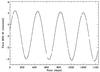 |
Fig. B.1 Kepler timing of KIC 3733735 modulo the median of its sampling rate Δt = 29.424389 min. |
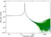 |
Fig. B.2 PSD of the same simulation as in Fig. 2 (black curve). The green curve is computed using an absolute regular grid of points in all the gaps. The light blue curve corresponds to the PSD calculated using a regular grid of points in the gaps in which the reference time for each gap is the last correct point. |
To properly interpolate the missing data one should take the sinusoidal variation in the time stamps into account. The first possibility consists of computing the BKJDTDB for each star of the field and for each quarter and use the corresponding time stamps for the interpolation. This solution is complicated and time consuming. There are three alternatives that could be easier, but not all provide good results. The first consists of computing an absolute regular grid of points with a sampling rate equal to the median of the original light curve, to replace the missing points. This is very fast but has the effect of mixing two different temporal sequences (a regular and an irregular). The resultant PSD is convolved by a new spectral window (Fig. B.2). The second possibility is to take a regular grid of points in the gaps but using as the reference time for each gap the one of the previous correct point. In a such way, we break the regularity in the time basis of the gaps and the increase of noise in the PSD is negligible (Fig. B.2). Finally, the third approach is the one followed in this paper and consists of converting the Kepler timing onto a regular grid of points and then interpolating the missing points into this regular grid. An example can be seen in Fig. 2. We have retained this option because this allows us to use the inpainting algorithm that works much faster on regular sampled time series because it takes advantage of the fast Fourier transforms.
All Tables
Background parameters of six red giants and eight solar-like stars (separated by a horizontal line) for the two types of datasets (with gaps “std” and the inpainted data “inp”).
All Figures
|
Fig. 1 Duration of observations (blue bars) and data gaps (yellow bars) during the 47 “Kepler months”, from Q0 to Q16. The Kepler scientific observations started on May 2, 2009 at 00:55 UT time. |
| In the text | |
|
Fig. 2 Spectral windows of the gaps induced by the angular momentum dump (AMD, top) and the downlink Earth pointing (DEP, bottom), respectively. |
| In the text | |
|
Fig. 3 Power spectral density (PSD) on logarithmic scale of a 2 μHz ideal sine wave (black) following the Barycentric Kepler Julian Date (BKJD, see Appendix A for further details). The red curve corresponds to the PSD of the same sine wave multiplied by the Kepler window function. Both PSDs were computed using a Lomb-Scargle algorithm. The blue line is the PSD resulting from converting the timing BKJD of the ideal sine wave (without gaps) into a regular grid and computed using a FFT. |
| In the text | |
|
Fig. 4 Top: PSD on logarithmic scale of KIC 2305930 smoothed using a 3-point boxcar function. The black curve corresponds to the original light curve. The pink curve is the PSD after correcting all the gaps with sizes less than 1 h (two long-cadence points), while the blue curve is the PSD after inpainting all the gaps less than 20 days. Bottom: ratio between the interpolated PSDs and the one with all the gaps. Both curves have been smoothed using a 300 point boxcar function. |
| In the text | |
|
Fig. 5 Long cadence light curve of KIC 3733735 (black) for quarters Q7 and Q8. The limit of the quarters are indicated by vertical blue dotted lines. The red line corresponds to the inpainted segments. |
| In the text | |
|
Fig. 6 As in Fig. 4, but for the evolved red giant KIC 8905990. In black the PSD for the original Kepler time series, while in blue is the inpainted one. Bottom panel: ratio between both PSDs. |
| In the text | |
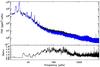 |
Fig. 7 Same as Fig. 6 but for the young F star KIC 3733735. |
| In the text | |
|
Fig. 8 Results of the background fits as describe in the text for three red giants (left panels) and three solar-like stars smoothed over 10 bins (right panels). Spectra obtained from gapped data are shown in black, while spectra after inpainting the light curves are in blue. The background fits are represented in red (resp. green) for the data with gaps (resp. inpainted data). |
| In the text | |
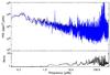 |
Fig. 9 Same as Fig. 6 but for the classical pulsator KIC 5892969. |
| In the text | |
|
Fig. 10 Zoom of the PSD shown in Fig.9 for a region of the PSD between 54 and 66 μHz. The top panel corresponds to the original PSD, and the bottom panel is the PSD obtained from the inpainted light curve (in blue). Vertical arrows mark new peaks found with this analysis. |
| In the text | |
|
Fig. B.1 Kepler timing of KIC 3733735 modulo the median of its sampling rate Δt = 29.424389 min. |
| In the text | |
|
Fig. B.2 PSD of the same simulation as in Fig. 2 (black curve). The green curve is computed using an absolute regular grid of points in all the gaps. The light blue curve corresponds to the PSD calculated using a regular grid of points in the gaps in which the reference time for each gap is the last correct point. |
| In the text | |
Current usage metrics show cumulative count of Article Views (full-text article views including HTML views, PDF and ePub downloads, according to the available data) and Abstracts Views on Vision4Press platform.
Data correspond to usage on the plateform after 2015. The current usage metrics is available 48-96 hours after online publication and is updated daily on week days.
Initial download of the metrics may take a while.