| Issue |
A&A
Volume 568, August 2014
|
|
|---|---|---|
| Article Number | A58 | |
| Number of page(s) | 16 | |
| Section | Atomic, molecular, and nuclear data | |
| DOI | https://doi.org/10.1051/0004-6361/201322937 | |
| Published online | 14 August 2014 | |
THz spectroscopy and first ISM detection of excited torsional states of 13C-methyl formate⋆
1
Laboratoire de Physique des Lasers, Atomes, et Molécules, UMR CNRS 8523,
Université Lille I,
59655
Villeneuve d’Ascq Cedex
France
e-mail:
This email address is being protected from spambots. You need JavaScript enabled to view it.
2
Departamento de Física Aplicada Unidad Asociada CSIC, Facultad de
Ciencias Experimentales, Universidad de Huelva, 21071
Huelva,
Spain
3
Centro de Astrobiología (CSIC-INTA), Department of Astrophysics.
Ctra de Ajalvir, 28850 Torrejón de
Ardoz, Madrid,
Spain
4
Laboratoire Interuniversitaire des Systèmes Atmosphériques, UMR
CNRS/IPSL 7583, Université Paris 7 et Université Paris Est,
61 Av. Charles de
Gaulle, 94010
Créteil Cedex,
France
5
Institut des Sciences Chimique de Rennes, École Nationale
Supérieure de Chimie de Rennes, CNRS, UMR 6226, Allée de Beaulieu, CS 50837, 35708
Rennes Cedex 7,
France
Received:
29
October
2013
Accepted:
24
April
2014
Abstract
Context. An astronomical survey of interstellar molecular clouds needs a previous analysis of the spectra in the microwave and sub-mm energy range of organic molecules to be able to identify them. We obtained very accurate spectroscopic constants in a comprehensive laboratory analysis of rotational spectra. These constants can be used to predict the transitions frequencies very precisely that were not measured in the laboratory.
Aims. We present the experimental study and its theoretical analysis for two 13C-methyl formate isotopologues to detect these two isotopologues for the first time in their excited torsional states, which lie at 130 cm-1 (200 K) in Orion-KL.
Methods. New spectra of HCOO13CH3 (13C2) methyl formate were recorded with the mm- and submm-wave spectrometer in Lille from 50 to 940 GHz. A global fit for vt = 0 and 1 was accomplished with the BELGI program to reproduce the experimental spectra with greater accuracy.
Results. We analysed 5728 and 2881 new lines for vt = 0 and 1 for HCOO13CH3. These new lines were globally fitted with 846 previously published lines for vt = 0. In consequence, 52 parameters of the RAM Hamiltonian were accurately determined and the value of the barrier height (V3 = 369.93168(395) cm-1) was improved. We report the detection of the first excited torsional states (vt = 1) in Orion-KL for the 13C2 and 13C1 methyl formate based on the present analysis and previously published data. We provide column densities, isotopic abundances, and vibrational temperatures for these species.
Conclusions. Following this work, accurate prediction can be provided. This permits detecting 135 features of the first excited torsional states of 13C-methyl formate isotopologues in Orion-KL in the 80−280 GHz frequency range, without missing lines.
Key words: line: identification / astronomical databases: miscellaneous / ISM: molecules / submillimeter: ISM / astrochemistry / ISM: individual objects: Orion KL
Full Table A.1 and the IRAM spectra as FITS files are only available at the CDS via anonymous ftp to cdsarc.u-strasbg.fr (130.79.128.5) or via http://cdsarc.u-strasbg.fr/viz-bin/qcat?J/A+A/568/A58
© ESO, 2014
1. Introduction
Methyl formate is one of the most abundant complex organic molecules in the interstellar medium (ISM). It was identified in different sources since 1975 (Brown et al. 1975; Churchwell et al. 1975); nearly one thousand lines were detected in the ground-torsional state vt = 0. Its abundance is particularly high in Orion-KL: it was detected up to 900 GHz (Comito et al. 2005) far from the maximum of absorption situated around 300 GHz; some lines from the first (Kobayashi et al. 2007), and more recently, lines from the second torsional state were detected (Takano et al. 2012). The abundance is also fairly high in W51e2, where lines from methyl formate in its first torsional states were found (Demyk et al. 2008). Molecules in the ISM can be used to probe the physical conditions of sources, as illustrated recently by Favre et al. (2011, 2014) using methyl formate to probe the temperature structure and spatial distribution of this species in Orion-KL; depending on the molecular species, the distribution of the molecular gas can be different in this source because of its complexity (which is a result of massive star formation processes) different cloud components coexist there. Organic saturated O-rich molecules such as methyl formate generally trace the compact ridge component (for a description of the different cloud components of Orion-KL see e.g. Blake et al. 1987; Schilke et al. 2001; Persson et al. 2007; Tercero et al. 2010, 2011; Neill et al. 2013).
Around 180 molecules have been detected in the ISM or circumstellar shells, but in high mass-forming regions such as Orion-KL, 30% of the lines remain unidentified (Esplugues et al. 2013a; Tercero et al. 2010). Its important to identify all the lines from the most abundant species. These molecules are often called “weeds”, and methyl formate is one of them. Identifying them is necessary in order to discover new species in the ISM without ambiguity. As shown recently by Tercero et al. (2013), the detection of methyl acetate (CH3COOCH3) and the gauche conformer of ethyl formate (g-CH3CH2OCOH) was only possible with the assignment of 4400 lines coming from several isotopologues and vibrational levels of different weeds: CH3CH2CN, CH2CHCN, HCOOCH3, and NH2CHO.
Most of the times, accurate spectroscopic data in the millimeter and submillimeter-wave domain are not available for the isotopologues and vibrational levels. While the normal species of methyl formate were extensively studied (Ilyushin et al. 2009, and references therein) of only the two commercially available isotopologues H13COOCH3 (Maeda et al. 2008a,b) and DCOOCH3 (Oesterling et al. 1995) were studied in the millimeter-wave region. Therefore we decided to investigate all the mono-isotopic species of methyl formate in the submillimeter-wave domain a few years ago. For each of them, this permits generating a new accurate prediction and allows detecting the 13C species (Willaert et al. 2006; Carvajal et al. 2007, 2009, 2010), DCOOCH3 (Margulès et al. 2010), 18O species (Tercero et al. 2012) in Orion-KL and recently HCOOCH2D (Coudert et al. 2013). This confirms the assumption that most of the U-lines come from known molecules. The lines detected for the 18O species gave us the idea that it might also be possible to find lines related to the first excited torsional states that lie at 130 cm-1 (200 K) of the most abundant isotopologues 13C.
Our motivations for studying of the first excited torsional state of HCOO13CH3 is also linked to a spectroscopic interest. Methyl formate, like other complex molecules, exhibits large-amplitude motion: torsion of the methyl group related to the rest of the molecules. A specific code that takes into account the interaction of the torsion and the overall rotation of the molecule is needed. Most of the codes were developed to treat data in the centimeter not in millimeter-wave domain. Recent efforts from different theoretical groups were recently make to improve the codes to reproduce the experimental accuracies with high quantum numbers that are reached at submillimeter frequencies. As shown for the normal species (Ilyushin et al. 2009) and the 13C1 species (Carvajal et al. 2010), the global treatment of the ground- and first torsional states permits removing the high correlation between torsional parameters. This improves the quality of the fit and finally the accuracy of the predictions for the two states.
These works permit the first detection of the excited torsional state of the two 13C-methyl formate isotopologues. As in Carvajal et al. (2009), we publish the spectroscopic work about HCOO13CH3 and the detection of the two 13C isotopologues in Orion together. In the previous paper about 13C2 (Carvajal et al. 2009), our measurements were limited to 660 GHz for the ground-torsional states. To provide an accurate prediction of this state in the ALMA range, we also reinvestigated this state up to 940 GHz.
2. Experiments
2.1. Synthesis of the methyl formate isotopologue HCOO13CH3
The details about synthesis and identification by NMR spectroscopy were described in Carvajal et al. (2009).
2.2. Lille – submillimeter spectra
The millimeter- and submillimeter-wave spectra were recorded using the Lille spectrometer that is based on solid-state sources (Motiyenko et al. 2010; Haykal et al. 2013a). The sample pressure was in the range 20−30×10-6 bars. Spectra were recorded at room temperature (T = 294 K) in the 150−210, 225−315, 400−500, 500−630, and 780−940 GHz regions with frequency steps of 30, 36, 48, 54, and 76 kHz and an acquisition time of 35 ms per point. Absorption signals were detected either by a Schottky diodes detector (Virginia Diodes Inc.) below 315 GHz or by an InSb liquid He-cooled bolometer (QMC Instruments Ltd.) above 400 GHz, and were processed on a computer. The absolute accuracy of the line-centre frequency is estimated to be better than 30 kHz (50 kHz above 700 GHz) for isolated lines and can be as low as 100 kHz (150 kHz above 700 GHz) for blended or very weak lines.
3. Assignments and fit of the HCOO13CH3 spectrum
The theoretical model and the so-called RAM method (rho-axis method) used for the present spectral analyses and fits of the ground- and first torsional-excited states of HCOO13CH3 species have also been used previously for a number of molecules that contain an internal methyl rotor (see for example Ilyushin et al. 2003, 2008) and in particular for the normal species of the cis-methyl formate (Carvajal et al. 2007; Ilyushin et al. 2009), the two 13C species (Carvajal et al. 2009, 2010), for DCOOCH3 (Margulès et al. 2010), and for 18O species (Tercero et al. 2012). The RAM Hamiltonian we used is based on previous works (Kirtman 1962; Lees & Baker 1968; Herbst et al. 1984). Because this method has been presented in great detail in the literature (Lin & Swalen 1959; Hougen et al. 1994; Kleiner 2010), we do not describe it here. The principal advantage of the RAM general approach used in our code BELGI, which is publicly available1, is its general approach that simultaneously takes into account the A- and E-symmetry states in our fit. All the torsional levels up to a truncation limit of vt = 8 are carefully tested and the interactions within the rotation-torsion energy levels are also included in the rotation-torsion Hamiltonian matrix elements (Kleiner et al. 1996). The various rotational, torsional, and coupling terms between rotation and torsion that we used for the fit of the HCOO13CH3 species were defined previously for the normal methyl formate species (Carvajal et al. 2007). The labelling scheme of the energy levels and transitions used for methyl formate was also described in the same reference, as was the connection with the more traditional JKa,Kc labelling.
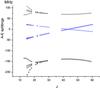 |
Fig. 1 A-E splitting of selected branches (R branches for Ka = 0;1 in blue and 1;2 in black) for vt = 1. The x-axis represents the situation without perturbation. The A transitions (▽ signs) are twice as far as the E transitions (+ signs). For Ka = 0;1 the A-E splitting changes sign at J = 44 (Ilyushin et al. 2009). |
We started with the assignment of the ground state. Predictions were provided by the BELGI program based on the set of 27 parameters previously determined in Carvajal et al. (2009). In this reference, only 658 lines were assigned from 150 to 700 GHz. Our new spectrometer has a wider coverage range than that used in 2009. Based on the previous work, we easily assigned the spectra up to J = 63 and Ka = 34 in the range 75−630 GHz. In the highest frequency range of the mm- and submm- wave spectrometer (700−940 GHz), the assignment was tentative because of the shift of the predicted lines from the experimental lines. The upper limit in frequency of the 936 previously fitted lines was 700 GHz. As a result, we assigned for the ground-state 5728 lines up to J = 60 and Ka = 35 from 50 to 940 GHz. Next, we started up again, but simultaneously including data of states vt = 0 and vt = 1. The fit was carried out in these two steps to avoid any possible misassignments. The improvement of the fit is then based on the variety and richness of the data set, and the addition of lines belonging to vt = 1 is crucial. The analysis of the first excited torsional state was challenging because of a larger splitting of the A and E component by the tunnelling effect. In a recent work by Tudorie et al. (2012) the band origins (EA = 132.4303 cm-1 and EE = 131.8445 cm-1) for vt = 1 of the parent molecule were precisely determined by a combination of microwave, mm-wave, submm-wave, and far infrared data. The value of height of the barrier was as much improved and V3 was determined to be equal to 370.7398 (58) cm-1. In this work, for HCOO13CH3, the first torsional excited substates are predicted to be EA = 131.0565 cm-1 and EE = 130.4856 cm-1. We estimated the rotational parameters using the same difference of the ground- and the first-torsional excited states rotational parameters of the 12C species. In the assignment procedure, the a-type transitions with A symmetry of R-branches were first analysed, in particular, the most intense lines with Ka = 0 and 1.
Methyl formate is a fairly asymmetric near-prolate top for which the dipole moment is non-zero along the a and b principle axis. For the parent specie, μa and μb were measured by Margulès et al. (2010) and their values are 1.648(8) and 0.706(12) D. We tracked these transitions based on the intensity criterion. Next we assigned the E type of transitions with the same benchmarks as those adopted for the A type of transitions. For Ka the splitting between the A transitions, as well as between the E transitions, decreases with the increase of the J quantum number. Four μa and μb rotational transitions with the same symmetry (A or E) become blended at J = 24. Furthermore, in the mm-wave ranges the splitting between the A and E transitions decreases with the increase of J and at a specific value of J in the submm-wave ranges this splitting changes sign (Fig. 1). Following this behaviour of the A and E type of transition for Ka = 0 and 1, we assigned them up to J = 50 at ~520 GHz. We fitted these for vt = 1 with the ERHAM (Groner 1997, 2012) program. The predictions based on this first fit were accurate enough to continue and to search for higher quantum number lines. We collected 800 A lines and 596 E lines with Ka,max = 19 and 11 up to J = 50 for the A and E lines. ERHAM2 treats each torsional state separately, and to proceed with the global analysis of vt = 0 and 1, we used BELGI. The final data set with the upper limits of the quantum numbers and the experimental uncertainties are summarized in Table 1. The 6574 lines belonging to vt = 0 and 2881 lines belonging to vt =1 were fitted with root-mean-square deviations of 38.3 and 41.9 kHz. The fit of the total of 9455 lines for vt = 0 and 1 of A and E symmetries resulted in the determination of 52 parameters of the RAM Hamiltonian. Table 3 presents the values of the set of 52 newly determined parameters. In this table we also provide a comparison with the previous work. Principally, we note a striking change in the value of the barrier height. The value of the parameter V3 changed from 407.1549(147) to 369.93168(395) cm-1.
The reason for this is the fact that this parameter is an effective value. In the previous
fit (Carvajal et al. 2009), the data set of lines
concerned only the vt = 0 state and,
therefore, neither the second-order parameter (V6) of the torsional potential function
nor the kinetic parameter F could be determined. Then, F was fixed to a relatively
high value estimated by ab initio methods, and in the fitting procedure, the effective value
of V3 absorbed the error of F and contained the
contribution of V6:
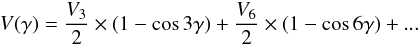 (1)The
new combination of data from vt = 0 and 1 improved
the quality of the fit and allowed determining of 25 new parameters, particularly
F and
V6.
(1)The
new combination of data from vt = 0 and 1 improved
the quality of the fit and allowed determining of 25 new parameters, particularly
F and
V6.
Torsion-rotation parameters needed for the global fit of transitions involving vt = 0 and vt = 1 torsional energy levels of 13C2-methyl formate (H12COO13CH3) provided in this work and comparison with the torsion-rotation parameters obtained in the former global fit of transitions only involving vt = 0 torsional states (Carvajal et al. 2009).
Rotational constants in the principal axis system (PAM), angles between the principal axis and the methyl top axis, and internal rotation parameters upon isotopic substitution.
Kinematic parameters and physical conditions of the Orion-KL spatial components.
4. Line strengths
The intensity calculations for the two 13C species of methyl formate were performed using the same
method described in Hougen et al. (1994) and Ilyushin et al. (2008), that was applied for the normal
species by Carvajal et al. (2007), the 13C species (Carvajal et al. 2009, 2010),
DCOOCH3 (Margulès et al. 2010), and 18O species (Tercero et al. 2012). For this reason we do not repeat it here. The line
strength calculation for the 13C species was performed using the same value for the dipole
moment as for the parent methyl formate (Margulès et al.
2010). This assumption was made because the angle between the internal axis of the
methyl top and the principal a-axis does not change much upon substitution (see the
<(i,a) angle values in Table 3). All other structural parameters such as the angle between RAM and PAM
axes (θRAM) and the ρ parameter do not change
much upon substitution (see Table 3). Because the
changes in the structure in the various isotopomers are not important, we assumed that the
dipole moment does not change considerably from one species to another. The dipole moment
components of H13COOCH3 (Carvajal et al.
2010) and HCOO13CH3 in RAM axis system that we used for the intensity
calculations are  D;
D;
 D and
D and
 D;
D;
 D, respectively. We provide
Table A.1, which is part of the supplementary Table S (available on CDS). It contains all
included lines from our fit for the HCOO13CH3 methyl formate species. They show the line assignments, the
observed frequencies with measurement uncertainty (in parenthesis), the computed
frequencies, observed-calculated values, the line strength, and the lower-state energy
relative to the J =
K = 0 A-species level taken as zero-energy level. The
prediction line-list of all transitions in vt = 0 and 1 will be
transmitted to the SPLATALOG and CDMS database (available at www.splatalogue.net).
D, respectively. We provide
Table A.1, which is part of the supplementary Table S (available on CDS). It contains all
included lines from our fit for the HCOO13CH3 methyl formate species. They show the line assignments, the
observed frequencies with measurement uncertainty (in parenthesis), the computed
frequencies, observed-calculated values, the line strength, and the lower-state energy
relative to the J =
K = 0 A-species level taken as zero-energy level. The
prediction line-list of all transitions in vt = 0 and 1 will be
transmitted to the SPLATALOG and CDMS database (available at www.splatalogue.net).
5. Detection of 13C-HCOOCH3vt = 1 in Orion KL
In this section we use the notation 13C-HCOOCH3 when we refer to the two isotopologues. Following the procedure of our previous papers, we searched for the present species in the molecular line survey of Orion KL performed with the IRAM 30 m telescope. We detected both 13C isotopologues of methyl formate in their first vibrationally excited state. In Sect. 5.1 we summarize the observations, data reduction, and overall results of this survey. We present the new detection in Sect. 5.2. In Sect. 5.3 we explain the assumed model and the excitation and radiative transfer calculations for vibrationally excited 13C and 12C methyl formate. We also compute our obtained 12C/13C ratio and the vibrational temperature for 13C-HCOOCH3vt = 1.
5.1. Observations, data reduction, and overall results
The molecular line survey towards Orion KL-IRc2 (α(J2000) = 5h35m14.5s, δ(J2000) = −5°22′30.0″) was performed between September 2004 and January 2007 in five observing sessions with the IRAM 30 m telescope. All frequencies allowed by the A, B, C, and D receivers were covered (80−115.5, 130−178, and 197−281 GHz) with a spectral resolution of 1−1.25 MHz. System temperatures, image side-band rejections, and half-power beam widths were in the ranges 100−800 K, 27−13 dB, and 29–9′′, from 80 to 281 GHz. The observations were performed in the balanced wobbler-switching mode. Pointing and focus were checked every 1−2 h on nearby quasars. The intensity scale was calibrated with two absorbers at different temperatures using the ATM package (Cernicharo 1985; Pardo et al. 2001).
The data were processed using the GILDAS software3.
The data reduction consisted of removing lines from the image side-band and fitting and
removing baselines. We observed each frequency setting twice, with the second one shifted
in frequency by 20 MHz. This allowed us to remove lines from the image side-band down to a
level of 30 dB (this means that lines in the image side-band of 30 K will contribute with
less than 0.03 K to the final reduced spectrum). Figures are shown in units of main-beam
antenna temperature,  /ηMB, where
ηMB is the main-beam efficiency ranged
from 0.82 to 0.48 from the lowest to the highest frequencies. For a detailed description
of the observations and data reduction procedures see Tercero et al. (2010).
/ηMB, where
ηMB is the main-beam efficiency ranged
from 0.82 to 0.48 from the lowest to the highest frequencies. For a detailed description
of the observations and data reduction procedures see Tercero et al. (2010).
Up to date, we performed a deep analysis of the data (15 papers have been already published): identifying more than 15 000 spectral features (Tercero et al. 2010; Tercero 2012), detecting new molecules in space (CH3COOCH3 and g-CH3CH2OCOH in Tercero et al. 2013; NH3D+ in Cernicharo et al. 2013; CH3CH2SH in Kolesniková et al. 2014; also tentative detections of c-C6H5O in Kolesniková et al. 2013 and upper limit calculations for the column density of non detected molecules −cis-CH2CHCH2CN and cis-CH2CHCH2NC− in Haykal et al. 2013b) and several new isotopologues and vibrationally excited states of well-known molecules in this source (13C-CH3CH2CN in Demyk et al. 2007; 13C-HCOOCH3 in Carvajal et al. 2009; CH3CH215N, CH3CHDCN, and CH2DCH2CN in Margulès et al. 2009; DCOOCH3 in Margulès et al. 2010; 18O-HCOOCH3 in Tercero et al. 2012; NH2CHO ν12 = 1 in Motiyenko et al. 2012; CH3CH2CN ν10 = 1 and ν12 = 1 in Daly et al. 2013; HCOOCH2D in Coudert et al. 2013; CH2CHCN ν10 = 1 ⇔ (ν11 = 1, ν15 = 1) in López et al. 2014), and constraining physical and chemical parameters by means of the analysis of different families of molecules (OCS, CS, H2CS, HCS+, CCS, CCCS species in Tercero et al. 2010; SiO and SiS species in Tercero et al. 2011; CH3CH2CN species in Daly et al. 2013; SO and SO2 species in Esplugues et al. 2013a; HC3N and HC5N species in Esplugues et al. 2013b; CH3CN in Bell et al. 2014; CH2CHCN species and the isocyanides in López et al. 2014). In addition and to analyze some of these results, we modelese the following molecules: CH3SH, CH3OH, CH3CH2OH in Kolesniková et al. (2014), HCOOCH3 in Margulès et al. (2010), and NH2CHO in Motiyenko et al. (2012). Nevertheless, the study of this line survey is still open and several groups are working simultaneously based on the scope of these observations4.
In agreement with numerous works of this region (see e.g. Blake et al. 1987; Schilke et al. 2001; Persson et al. 2007; Neill et al. 2013), at least four cloud components could be identified in the line profiles of our low-resolution spectral lines, which are characterized by different radial velocities and line widths (Tercero et al. 2010, 2011). Each component corresponds to specific region of the cloud that overlaps in our telescope beam. Table 4 summarizes the kinematic and physical parameters of the different components in Orion-KL.
Detected lines of 13C-HCOOCH3vt = 1 towards Orion KL.
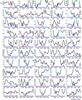 |
Fig. 2 Selected lines of A/E-H13COOCH3vt = 1 (modelled in red) and A/E-HCOO13CH3vt = 1 (modelled in dark blue) toward Orion-IRc2. The continuous cyan line corresponds to all lines already modelled in our previous papers except H13COOCH3 and HCOO13CH3νt = 1 (see Sect. 5.1). A vLSR of 7 km s-1 is assumed. |
5.2. Results
The two 13C
isotopologues of HCOOCH3 in their first vibrationally excited state
(vt = 1) have been
detected in Orion-KL by means of 135 spectral features (77 of them practically unblended)
without missing transitions in the range 80−280 GHz. Figure 2 shows selected
detected lines of the two isotopologues together with our best model (see below). The
black histogram line corresponds with the observed spectra. The model of the
H13COOCH3vt = 1 and
HCOO13CH3νt = 1 lines is shown
in red and dark blue, respectively. In all boxes unblended or slightly blended detected
lines of these species are depicted. The cyan blue line represents the total model
compiled from our already published work (see Sect. 5.1). In Table 5 we list all detected
features in our line survey. These detections are based on an inspection of the data and
the modelled synthetic spectrum of the studied species and all the species already
identified in our previous papers (see above). The observed main-beam temperature and the
radial velocity where obtained from the peak channel of our spectra, therefore, errors in
the baselines −up to
±0.15 K for spectra at
1.3 mm due to the extremely high line density (line confusion limit) − and contribution from other species might
affect the  value.
Adding species to our total model allows reducing the uncertainty in the baselines, so, in
general, the has to be
considered as the total intensity of the detected feature and an upper limit for the
intensity of the methyl formate species in this study. Nevertheless, in Table 5 we found some values of the
lower
than those predicted by the model (synthetic spectrum HCOO13CH3 and H13COOCH3νt =
1); uncertainties in the removed baselines are the most probable source
for these discrepancies. The uncertainty in the radial velocity was adopted from the
spectral resolution of our data. Most unblended detected lines show a radial velocity of
≃7 km s-1, in agreement with the
expected velocity for emission from the compact ridge component where organic saturated
O-rich molecules have the largest abundances inside the region. In addition, most detected
lines of methyl formate, its isotopologues, and its first vibrationally excited state
appear at the same radial velocity (see e.g. Carvajal et
al. 2009; Margulès et al. 2010; Favre et al. 2011; Tercero et al. 2012; López et al., in prep.).
value.
Adding species to our total model allows reducing the uncertainty in the baselines, so, in
general, the has to be
considered as the total intensity of the detected feature and an upper limit for the
intensity of the methyl formate species in this study. Nevertheless, in Table 5 we found some values of the
lower
than those predicted by the model (synthetic spectrum HCOO13CH3 and H13COOCH3νt =
1); uncertainties in the removed baselines are the most probable source
for these discrepancies. The uncertainty in the radial velocity was adopted from the
spectral resolution of our data. Most unblended detected lines show a radial velocity of
≃7 km s-1, in agreement with the
expected velocity for emission from the compact ridge component where organic saturated
O-rich molecules have the largest abundances inside the region. In addition, most detected
lines of methyl formate, its isotopologues, and its first vibrationally excited state
appear at the same radial velocity (see e.g. Carvajal et
al. 2009; Margulès et al. 2010; Favre et al. 2011; Tercero et al. 2012; López et al., in prep.).
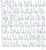 |
Fig. 3 Selected lines of A/E-HCOOCH3νt = 1 (modelled in dark blue) toward Orion-IRc2. The dashed red line and the green continuous line correspond to methyl formate in the ground state and the sum of the emission of vt = 1 and vt = 0, respectively. The continuous cyan line corresponds to all lines already modelled in our previous papers except HCOOCH3νt = 0, 1 (see Sect. 5.1). A vLSR of 9 km s-1 is assumed. The x-axis is the frequency in GHz. |
5.3. Modelling the data
To model the emission of H13COOCH3 and HCOO13CH3νt = 1 we used an excitation and radiative transfer code: MADEX (Cernicharo 2012). This time we applied LTE conditions because we lacked collisional rates for these species. Two compact ridge components (vLSR = 7 km s-1 and Δv = 3 km s-1) are enough to model the line profiles: one at 110 K, with diameter of 15′′, and a column density of (6±3)×1013 cm-2 for each state (A and E) of each isotopologue, and a hotter and inner compact ridge at 250 K with a diameter of 10′′, and a column density of (6±3)×1014 cm-2 for each state (A and E) of each isotopologue (both components are 7′′ offset from the pointing position; interferometric maps show this component offset ≃7′′ southwest from the source I− located 0.5′′ south of IRc2, Menten & Reid 1995; see e.g. Neill et al. 2013 for ALMA cycle 0 maps). The beam dilution for each line (depending on the frequency) has been also taken into account in the calculation of the emerging line intensities. The obtained synthetic spectra is shown in Fig. 2. We obtained source averaged-column densities over the source size given for each component. Uncertainties of the column density results were estimated to be between 20−30% for this line survey (see Tercero et al. 2010) taking into account errors introduced by different sources, such as the spatial overlap of the different cloud components, the modest angular resolution, or pointing errors. Nevertheless, high overlap problems add another source of uncertainty (rising to 50%) for results obtained by means of weak lines such as those of H13COOCH3 and HCOO13CH3vt = 1. All together we obtained a total column density of (1.4±0.7)×1015 cm-2 for each 13C isotopologue of vibrationally excited methyl formate.
5.3.1. Isotope ratios
To obtain the 12C/13C ratio, we included our model for A/E-HCOOCH3vt = 1 (López et al., in prep.). Figure 3 shows selected lines of methyl formate in its first vibrationally excited state in the 2 mm window (from 130 to 178 GHz). We modelled these species assuming all components listed in Table 4 and the hotter and inner compact ridge described above. The differences between the considered components with respect to the model of the 13C isotopologues arise because the much more stronger lines of the main isotopologue in all the spectral band (from 80 to 280 GHz) allow us to distinguish the contribution of several cloud components in the line profiles, although some of them, such as the plateau contribution, are very low. For HCOOCH3vt = 1 we obtained a total column density of (1.9±0.6)×1016 cm-2.
The column density ratio between the two vibrationally excited isotopologues (main and 13C) of methyl formate yields a 12C/13C ratio between 6−35 (considering the error bars and assuming the same partition function for both species). Taking into account the weakness of the 13C lines, the derived ratios are compatible with the value of 12C/13C ≃ 35 obtained with the column density ratios between 13C-HCOOCH3 and HCOOCH3 in the ground state (see Carvajal et al. 2009; Margulès et al. 2010) and agrees quite well with previous results of this ratio in Orion KL (Johansson et al. 1984; Blake et al. 1987; Demyk et al. 2007; Tercero et al. 2010; Daly et al. 2013; Esplugues et al. 2013b).
5.3.2. Vibrational temperatures
We can estimate vibrational temperatures
from (2)where
Eνt =
1 is the energy of the vibrational state (187.6 K),
Tvib is the vibrational temperature,
fν is the vibrational
partition function, N(13C-HCOOCH3vt = 1) is the column
density of the vibrational state, and N(13C-HCOOCH3) is the total column density of 13C methyl formate. Taking into
account that N(13C-HCOOCH3) = N(ground) ×
fν and assuming the same
partition function for these species in the ground- and the first vibrationally excited
states, we only need the energy of the vibrational state and the column densities of
13C-HCOOCH3vt = 1 and
13C-HCOOCH3vt = 0 to derive the
vibrational temperatures.
(2)where
Eνt =
1 is the energy of the vibrational state (187.6 K),
Tvib is the vibrational temperature,
fν is the vibrational
partition function, N(13C-HCOOCH3vt = 1) is the column
density of the vibrational state, and N(13C-HCOOCH3) is the total column density of 13C methyl formate. Taking into
account that N(13C-HCOOCH3) = N(ground) ×
fν and assuming the same
partition function for these species in the ground- and the first vibrationally excited
states, we only need the energy of the vibrational state and the column densities of
13C-HCOOCH3vt = 1 and
13C-HCOOCH3vt = 0 to derive the
vibrational temperatures.
In Carvajal et al. (2009) we did not consider the hotter component of the compact ridge for column density calculations. After several works on methyl formate (Carvajal et al. 2009; Margulès et al. 2010; Tercero et al. 2012; Coudert et al. 2013; López et al., in prep.) we realize that this hotter component plays an important role in the global analysis of this molecule. In Margulès et al. (2010) we introduced a hot compact ridge to model the lines of main isotopologue of the methyl formate to properly reproduce the line profiles. After that, the study of the vibrationally excited states (this work and A. López et al., in prep.) confirms that a hot compact ridge is needed to understand the emission of this molecule. Therefore, quite strong lines such as those of 13C-HCOOCH3 require the hot compact ridge component to obtain the best fit. Consequently, here we again modeled the emission from H13COOCH3 and HCOO13CH3 taking into account a compact ridge at a temperature of 250 K and a source size of 10′′. As in Carvajal et al. (2009), all cloud components of Table 4 where taken into account to reproduce the line profiles. Using MADEX and assuming LTE conditions, the obtained column densities for each 13C isotopologue and each state (A and E) are (2.0±0.6)×1015 cm-2 and (2.0 ± 0.6) × 1014 cm-2 for the T = 250 K compact ridge and the T = 110 K compact ridge, respectively, and (1.0±0.3) × 1013 cm-2 for the plateau, the extended ridge, and the hot core. These values yield a total column density of a factor 3 higher than obtained in Carvajal et al. (2009). This difference is mostly due to the reduced source size when we introduced the hotter component of the compact ridge.
At this point, we were ready to derive the vibrational temperatures. We assumed that both gases (ground-state and vibrationally excited) are spatially coincident, so the calculated vibrational temperatures have to be considered as lower limits. A Tvib = 156 K was obtained for H13COOCH3 and HCOO13CH3vt = 1 in each compact ridge component. This value is similar to the averaged kinetic temperature we adopted in this model (180 K). This result indicates that collisions are probably the main mechanism to populate the vibrationally excited levels of methyl formate.
6. Conclusion
We measured the spectra of HCOO13CH3 from 75 to 940 GHz. We analyzed 2881 lines from the first excited torsional states, 5728 new lines corresponding to the ground-vibrational states were also measured and added to the previous ones from Carvajal et al. (2009). The global fit of the 9455 lines, taking into account the internal rotation motion, was made using the rho-axis-method and the BELGI code. Fifty-two parameters could be determined, the global fit of both states permitted us to obtain uncorrelated values of the torsional parameters: F, V3, and V6. The value of barrier height (V3 = 369.93168(395) cm-1) has been significantly improved.
Owing to this work and Carvajal et al. (2009), accurate predictions of line positions and intensities were performed. In the line survey of Orion-KL with the IRAM 30 m telescope, this permits detecting 135 spectral features in the range 80−280 GHz; there are no missing transitions in this range. This is the first detection of an excited vibrational state of a methyl formate isotopologue.
At the beginning of the line identification process of this line survey (in 2005), nearly 8000 spectral features were U lines. In 2007 we began a close collaboration between astronomers and spectroscopists to reduce the uncertainty due to unidentified lines in spectral surveys. New isotopologues of ethyl cyanide and methyl formate (Demyk et al. 2007; Margulès et al. 2009, 2010; Carvajal et al. 2009; Tercero et al. 2012; Coudert et al. 2013) and new vibrationally excited states of formamide (Motiyenko et al. 2012), ethyl cyanide (Daly et al. 2013), and vinyl cyanide (López et al. 2014) have been studied in spectroscopy laboratories and detected in Orion KL for the first time space. Altogether, we reduced 3000 of unidentified lines through these studies. At this point, we were ready to search for new molecular species, detecting methyl acetate and gauche-ethyl formate (Tercero et al. 2013) and gauche-ethyl mercaptan (Kolesniková et al. 2014) for the first time in space, and providing the tentative detection of phenol (Kolesniková et al. 2013). These new species together with the work of López et al. (in prep., about vibrationally excited CH3OCOH and CH3COOH) account for ≃1000 lines. Up to date, we have reduced 4000 of U lines in the survey of Orion KL. We expect that a large number of the still unidentified lines arise from vibrationally modes of abundant species. However, low-lying vibrationally excited states of abundant molecules such as ethyl cyanide (for example the ν13 = 2 /ν21 = 2 state at ~420 cm-1) or methanol are still only poorly characterized in the laboratory, and certainly contribute to the remaining U-lines. The main goal of our studies is to provide the community with a fully analysed line survey of Orion that will constitute a template for ALMA observations of warm clouds.
The source code for the fit, an example of input data file, and a readme file are available at the web site (http://www.ifpan.edu.pl/~kisiel/introt/introt.htm#belgi) managed by Zbigniew Kisiel. Extended versions of the code made to fit transitions with higher J and K are also available from the authors (I. Kleiner and M.C.).
The data of the IRAM 30 m line survey of Orion KL are available in ascii format on request to B. Tercero.
Acknowledgments
M.C. acknowledges the financial support the Spanish Government through grant FIS2011-28738-C02-02, and by a joint project within the framework of a CNRS (France) and CSIC (Spain) agreement (Code No.: 2011 FR0018). J.C., A.L. and B.T. thank the Spanish MINECO for funding support from grants CSD2009-00038, AYA2009-07304, and AYA2012-32032. This work was supported by the Centre National d’Etudes Spatiales (CNES) and the Action sur Projets de l’INSU, “Physique et Chimie du Milieu Interstellaire”. This work was also performed under the ANR-08-BLAN-0054.
References
- Bell, T. A., Cernicharo, J., Viti, S., et al. 2014, A&A, 564, A114 [NASA ADS] [CrossRef] [EDP Sciences] [Google Scholar]
- Blake, G. A., Sutton, E. C., Masson, C. R., & Philips, T. H. 1987, ApJ, 315, 621 [NASA ADS] [CrossRef] [Google Scholar]
- Brown, R. D., Crofts, J. G., Gardner, F. F., et al. 1975, ApJ, 197, L29 [NASA ADS] [CrossRef] [Google Scholar]
- Churchwell, E., & Winnewisser, G. 1975, A&A, 45, 229 [NASA ADS] [Google Scholar]
- Carvajal, M., Willaert, F., Demaison, J., & Kleiner, I. 2007, J. Mol. Spectrosc., 246, 158 [Google Scholar]
- Carvajal, M., Margulès, L., Tercero, B., et al. 2009, A&A, 500, 1109 [NASA ADS] [CrossRef] [EDP Sciences] [Google Scholar]
- Carvajal, M., Kleiner, I., & Demaison, J. 2010, ApJS, 190, 315 [NASA ADS] [CrossRef] [Google Scholar]
- Cernicharo 1985, Internal IRAM report (Granada: IRAM) [Google Scholar]
- Cernicharo, J. 2012, in ECLA-2011: Proc. of the European Conf. Laboratory Astrophysics, EAS Publ. Ser., eds C. Stehl, C. Joblin, & L. d’Hendecourt (Cambridge: Cambridge Univ. Press), 251 [Google Scholar]
- Cernicharo, J., Tercero, B., Fuente, A., et al. 2013, ApJ, 771, L10 [NASA ADS] [CrossRef] [Google Scholar]
- Comito, C., Schilke, P., Phillips, T. G., et al. 2005, ApJS, 156, 127 [NASA ADS] [CrossRef] [Google Scholar]
- Coudert, L. H., Drouin, B. J., Tercero, B., et al. 2013, ApJ, submitted [Google Scholar]
- Curl, R. F. 1959, J. Chem. Phys., 30, 1529 [NASA ADS] [CrossRef] [Google Scholar]
- Daly, A. M., Bermúdez, C., López, A., et al. 2013, ApJ, 768, 81 [NASA ADS] [CrossRef] [Google Scholar]
- Demyk, K., Mäder, H., Tercero, B., et al. 2007, A&A, 466, 255 [NASA ADS] [CrossRef] [EDP Sciences] [Google Scholar]
- Demyk, K., Wlodarczak, G., & Carvajal, M. 2008, A&A, 489, 589 [NASA ADS] [CrossRef] [EDP Sciences] [Google Scholar]
- Esplugues, G. B., Tercero, B., Cernicharo, J. et al. 2013, A&A, 556, A143 [NASA ADS] [CrossRef] [EDP Sciences] [Google Scholar]
- Esplugues, G. B., Cernicharo, J., Viti, S., et al. 2013, A&A, 559, A51 [NASA ADS] [CrossRef] [EDP Sciences] [Google Scholar]
- Favre, C., Despois, D., Brouillet, N., et al. 2011, A&A, 532, A32 [NASA ADS] [CrossRef] [EDP Sciences] [Google Scholar]
- Favre, C., Carvajal, M., Field, D., et al. 2014, ApJ, submitted [Google Scholar]
- Groner, P. 1997, J. Chem. Phys., 107, 4483 [NASA ADS] [CrossRef] [Google Scholar]
- Groner, P. 2012, J. Mol. Spectrosc., 278, 52 [NASA ADS] [CrossRef] [Google Scholar]
- Haykal, I., Motiyenko, R. A., Margulès, L., & Huet, T. R. 2013a, A&A, 549, A96 [NASA ADS] [CrossRef] [EDP Sciences] [Google Scholar]
- Haykal, I., Margulès, L., Motiyenko, R. A., et al. 2013b, ApJ, 777, 120 [NASA ADS] [CrossRef] [Google Scholar]
- Herbst, E., Messer, J. K., De Lucia, F. C., & Helminger, P. 1984, J. Mol. Spectrosc., 108, 42 [Google Scholar]
- Hougen, J. T., Kleiner, I., & Godefroid, M. 1994, J. Mol. Spectrosc., 163, 559 [Google Scholar]
- Ilyushin, V., Alekseev, E. A., Dyubko, S. F., & Kleiner, I. 2003, J. Mol. Spectrosc., 220, 170 [Google Scholar]
- Ilyushin, V., Kleiner, I., & Lovas, F. J. 2008, J. Phys. Chem. Ref. Data, 37, 97 [NASA ADS] [CrossRef] [Google Scholar]
- Ilyushin, V. V., Kryvda, A., & Alekseev, E. 2009, J. Mol. Spectrosc., 255, 32 [Google Scholar]
- Johansson, L. E. B., Andersson, C., Elldér, J., et al. 1984, A&A, 130, 227 [NASA ADS] [PubMed] [Google Scholar]
- Kirtman, B. 1962, J. Chem. Phys., 37, 2516 [NASA ADS] [CrossRef] [Google Scholar]
- Kleiner, I. 2010, J. Mol. Spectrosc., 260, 1 [Google Scholar]
- Kleiner, I., Hougen, J. T., Grabow, J. U., et al. 1996, J. Mol. Spectrosc., 179, 41 [NASA ADS] [CrossRef] [Google Scholar]
- Kobayashi, K., Ogata, K., Tsunekawa, S., & Takano, S. 2007, ApJ, 657, L17 [NASA ADS] [CrossRef] [Google Scholar]
- Kolesniková, L., Daly, A. M., Alonso, J. L., Tercero, B., & Cernicharo, J. 2013, J. Mol. Spectrosc., 289, 13 [Google Scholar]
- Kolesniková, L., Tercero, B., & Cernicharo, J. 2014, ApJ, 784, L7 [NASA ADS] [CrossRef] [Google Scholar]
- Lees, R. M., & Baker, J. G. 1968, J. Chem. Phys., 48, 5299 [NASA ADS] [CrossRef] [Google Scholar]
- Lin, C. C., & Swalen, J. D. 1959, Rev. Mod. Phys., 31, 841 [NASA ADS] [CrossRef] [Google Scholar]
- López, A., Tercero, B., Kisiel, Z., et al. 2014, A&A, submitted [Google Scholar]
- Maeda, A., Medvedev, I. R., De Lucia, F. C., & Herbst, E. 2008a, ApJS, 175, 138 [NASA ADS] [CrossRef] [Google Scholar]
- Maeda, A., De Lucia, F. C., & Herbst, E. 2008b, J. Mol. Spectrosc., 251, 293 [Google Scholar]
- Margulès, L., Motiyenko, R. A., Demyk, K., et al. 2009, A&A, 493, 565 [NASA ADS] [CrossRef] [EDP Sciences] [Google Scholar]
- Margulès, L., Huet, T. R., Demaison, J., et al. 2010, ApJ, 714, 1120 [NASA ADS] [CrossRef] [Google Scholar]
- Menten, K. M., & Reid, M. J. 1995, ApJ, 445, L157 [NASA ADS] [CrossRef] [Google Scholar]
- Motiyenko, R. A., Margulès, L., Alekseev, E. A., Guillemin, J.-C., & Demaison, J. 2010, J. Mol. Spectrosc., 264, 94. [Google Scholar]
- Motiyenko, R. A., Tercero, B., Cernicharo, J., & Margulès, L. 2012, A&A, 548, A71 [NASA ADS] [CrossRef] [EDP Sciences] [Google Scholar]
- Neill, J. L., Crockett, N. R., Bergin, E. A., Pearson, J. C., & Xu, L.-H. 2013, ApJ, 777, 85 [NASA ADS] [CrossRef] [Google Scholar]
- Oesterling, L. C., Ferguson, D. W., Herbst, E., & De Lucia, F. C. 1995, J. Mol. Spectrosc., 172, 469 [Google Scholar]
- Pardo, J. R., Cernicharo, J., & Serabyn, E. 2001, IEEE Tras. Antennas and Propagation, 49, 12 [Google Scholar]
- Persson, C. M., Olofsson, A. O. H., Koning, N., et al. 2007, A&A, 476, 807 [NASA ADS] [CrossRef] [EDP Sciences] [Google Scholar]
- Schilke, P., Benford, C. J., Hunter, T. R., Lis, D. C., & Philips, T. G. 2001, ApJS, 132, 281 [NASA ADS] [CrossRef] [Google Scholar]
- Tercero, B. 2012, Ph.D., Univ. Complutense de Madrid [Google Scholar]
- Tercero, B., Pardo, J. R., Cernicharo, J. R., & Goicoechea, J. R. 2010, A&A, 517, A96 [NASA ADS] [CrossRef] [EDP Sciences] [Google Scholar]
- Tercero, B., Vincent, L., Cernicharo, J., Viti, S., & Marcelino, N. 2011, A&A, 528, A26 [NASA ADS] [CrossRef] [EDP Sciences] [Google Scholar]
- Tercero, B., Margulès, L., Carvajal, M., et al. 2012, A&A, 538, A119 [NASA ADS] [CrossRef] [EDP Sciences] [Google Scholar]
- Tercero, B., Kleiner, I., Cernicharo, J., et al. 2013, ApJ, 770, L13 [Google Scholar]
- Tudorie, M., Ilyushin, V., Van der Auwera, J., et al. 2012, J. Chem. Phys., 137, 064304 [NASA ADS] [CrossRef] [Google Scholar]
- Willaert, F., Møllendal, H., Alekseev, E., et al. 2006, J. Mol. Struct., 795, 4 [NASA ADS] [CrossRef] [Google Scholar]
- Takano, S., Sakai, Y., Kakimoto, S., Sasaki, M., & Kobayasho, K. 2012, PASJ, 64, 89 [NASA ADS] [Google Scholar]
Appendix A: Part of the supplementary tables available at the CDS
All Tables
Torsion-rotation parameters needed for the global fit of transitions involving vt = 0 and vt = 1 torsional energy levels of 13C2-methyl formate (H12COO13CH3) provided in this work and comparison with the torsion-rotation parameters obtained in the former global fit of transitions only involving vt = 0 torsional states (Carvajal et al. 2009).
Rotational constants in the principal axis system (PAM), angles between the principal axis and the methyl top axis, and internal rotation parameters upon isotopic substitution.
All Figures
|
Fig. 1 A-E splitting of selected branches (R branches for Ka = 0;1 in blue and 1;2 in black) for vt = 1. The x-axis represents the situation without perturbation. The A transitions (▽ signs) are twice as far as the E transitions (+ signs). For Ka = 0;1 the A-E splitting changes sign at J = 44 (Ilyushin et al. 2009). |
| In the text | |
|
Fig. 2 Selected lines of A/E-H13COOCH3vt = 1 (modelled in red) and A/E-HCOO13CH3vt = 1 (modelled in dark blue) toward Orion-IRc2. The continuous cyan line corresponds to all lines already modelled in our previous papers except H13COOCH3 and HCOO13CH3νt = 1 (see Sect. 5.1). A vLSR of 7 km s-1 is assumed. |
| In the text | |
|
Fig. 3 Selected lines of A/E-HCOOCH3νt = 1 (modelled in dark blue) toward Orion-IRc2. The dashed red line and the green continuous line correspond to methyl formate in the ground state and the sum of the emission of vt = 1 and vt = 0, respectively. The continuous cyan line corresponds to all lines already modelled in our previous papers except HCOOCH3νt = 0, 1 (see Sect. 5.1). A vLSR of 9 km s-1 is assumed. The x-axis is the frequency in GHz. |
| In the text | |
Current usage metrics show cumulative count of Article Views (full-text article views including HTML views, PDF and ePub downloads, according to the available data) and Abstracts Views on Vision4Press platform.
Data correspond to usage on the plateform after 2015. The current usage metrics is available 48-96 hours after online publication and is updated daily on week days.
Initial download of the metrics may take a while.