| Issue |
A&A
Volume 567, July 2014
|
|
|---|---|---|
| Article Number | A119 | |
| Number of page(s) | 19 | |
| Section | Extragalactic astronomy | |
| DOI | https://doi.org/10.1051/0004-6361/201423642 | |
| Published online | 25 July 2014 | |
ALMA-backed NIR high resolution integral field spectroscopy of the NUGA galaxy NGC 1433⋆,⋆⋆
1 I. Physikalisches Institut, Universität zu Köln, Zülpicher Str. 77, 50937 Köln, Germany
e-mail: This email address is being protected from spambots. You need JavaScript enabled to view it.
2 Max-Planck-Institut für Radioastronomie, auf dem Hügel 69, 53121 Bonn, Germany
3 Observatoire de Paris, LERMA, CNRS: UMR8112, 61 Av. de l’Observatoire, 75014 Paris, France
4 Observatorio Astronómico Nacional (OAN)-Observatorio de Madrid, Alfonso XII 3, 28014 Madrid, Spain
5 Deutsches Zentrum für Luft- und Raumfahrt (DLR), Königswinterer Str. 522-524, 53227 Bonn, Germany
Received: 14 February 2014
Accepted: 17 April 2014
Abstract
Aims. We present the results of near-infrared (NIR) H- and K-band European Southern Observatory SINFONI integral field spectroscopy (IFS) of the Seyfert 2 galaxy NGC 1433. We investigate the central 500 pc of this nearby galaxy, concentrating on excitation conditions, morphology, and stellar content. NGC 1433 was selected from our extended NUGA(-south) sample, which was additionally observed with the Atacama Large Millimeter/submillimeter Array (ALMA). NGC 1433 is a ringed, spiral galaxy with a main stellar bar in roughly east–west direction (PA 94°) and a secondary bar in the nuclear region (PA 31°). Several dusty filaments are detected in the nuclear region with the Hubble Space Telescope. ALMA detects molecular CO emission coinciding with these filaments. The active galactic nucleus is not strong and the galaxy is also classified as a low-ionization emission-line region (LINER).
Methods. The NIR is less affected by dust extinction than optical light and is sensitive to the mass-dominating stellar populations. SINFONI integral field spectroscopy combines NIR imaging and spectroscopy, allowing us to analyse several emission and absorption lines to investigate the stellar populations and ionization mechanisms over the 10″ × 10″ field of view (FOV).
Results. We present emission and absorption line measurements in the central kpc of NGC 1433. We detect a narrow Balmer line and several H2 lines. We find that the stellar continuum peaks in the optical and NIR in the same position, indicating that there is no covering of the center by a nuclear dust lane. A strong velocity gradient is detected in all emission lines at that position. The position angle of this gradient is at 155° whereas the galactic rotation is at a position angle of 201°. Our measures of the molecular hydrogen lines, hydrogen recombination lines, and [Fe ii] indicate that the excitation at the nucleus is caused by thermal excitation, i.e., shocks that can be associated with active galactic nuclei emission, supernovae, or outflows. The line ratios [Fe ii]/Paβ and H2/Brγ show a Seyfert to LINER identification of the nucleus. We do not detect high star formation rates in our FOV. The stellar continuum is dominated by spectral signatures of red-giant M stars. The stellar line-of-sight velocity follows the galactic field whereas the light continuum follows the nuclear bar.
Conclusions. The dynamical center of NGC 1433 coincides with the optical and NIR center of the galaxy and the black hole position. Within the central arcsecond, the molecular hydrogen and the 12CO(3−2) emissions – observed in the NIR and in the submillimeter with SINFONI and ALMA, respectively – are indicative for a nuclear outflow originating from the galaxy’s SMBH. A small circum-nuclear disk cannot be fully excluded. Derived gravitational torques show that the nuclear bar is able to drive gas inward to scales where viscosity torques and dynamical friction become important. The black hole mass, derived using stellar velocity dispersion, is ~107M⊙.
Key words: galaxies: active / galaxies: individual: NGC 1433 / galaxies: ISM / galaxies: kinematics and dynamics / galaxies: nuclei / infrared: galaxies
Based on the ESO-VLT proposal ID: 090.B-0657(A) and on observations carried out with ALMA in cycle 0.
Appendix A is available in electronic form at http://www.aanda.org
© ESO, 2014
1. Introduction
The NUclei of GAlaxies (NUGA) project (García-Burillo et al. 2003) started with the IRAM Plateau de Bure Interferometer (PdBI) and 30 m single-dish survey of nearby low-luminosity active galactic nuclei (LLAGN) in the northern hemisphere. The aim is to map the distribution and dynamics of molecular (cool) gas in the inner kpc of LLAGN and to study the possible mechanisms for gas fueling at high angular resolution (≈0.̋5−2″) and high sensitivity. The step-by-step implementation of the Atacama Large Millimeter/submillimeter Array (ALMA) in the Atacama desert in Chile finally allows the NUGA project to expand to the southern hemisphere at an even higher angular resolution (≈6−37 mas, assuming the use of the full array) and sensitivity. The Spectrograph for INtegral Field Observations in the Near Infrared (SINFONI; Eisenhauer et al. 2003; Bonnet et al. 2004) adds complementary information to the NUGA goal in the near-infrared (NIR). By mapping (hot-)gas and the mass dominating stellar population the fueling of nearby LLAGN can be investigated in the NIR.
1.1. Feeding and feedback in AGN
An active galactic nucleus (AGN), as a highly ionizing source, needs to show powerful highly ionizing emission coming from an unresolved region. This powerful emission ionizes the surrounding gas on scales from several lightdays (e.g., broad line region, BLR) to several hundreds of parsecs (e.g., narrow line region, NLR) and up to even larger scales via outflows and jets. Usually, a dust mantle surrounds the AGN on parsec to tens of parsec scales, inferred from high column densities toward Seyfert 2 AGN and dust black-body emission in Seyfert 1 AGN with temperatures up to the sublimation temperature of dust (~1300 K). The source of dust heating must be highly ionizing emission, probably originated by the accretion of gas onto a supermassive black hole (SMBH).
Tight correlations between the SMBH and its host galaxy, especially the bulge stellar velocity dispersion and luminosity have been found (e.g., Ferrarese & Merritt 2000; Magorrian et al. 1998). These correlations connect the mass, luminosity, and kinematics of the galactic bulge with the mass of the central SMBH. To feed an SMBH, the gas within the bulge needs to be transported toward the center. There are two ways to remove angular momentum in gas and consequently produce its infall. One way is through gravitational mechanisms that exert gravitational torques such as galaxy-galaxy interactions (e.g., galaxy merger) or non-axisymmetries within the galaxy potential (e.g., spiral density waves or stellar bars on large scales). It is also possible to remove angular momentum in gas through hydrodynamical mechanisms such as shocks and viscosity torques introduced by turbulences in the interstellar medium (ISM). The NUGA project has already studied the gaseous distribution in more than ten nearby galaxies (~4−40 Mpc). They show a variety of morphologies in nuclear regions, including bars and spirals (García-Burillo et al. 2005, 2009; Boone et al. 2007; Hunt et al. 2008; Lindt-Krieg et al. 2008), rings (Combes et al. 2004, 2009; Casasola et al. 2008) and lopsided disks (García-Burillo et al. 2003; Krips et al. 2005; Casasola et al. 2010). Gravitational torques, when present, are the strongest mechanism to successfully transport gas close to the nucleus, on smaller scales (<200 pc) viscosity torques can take over (e.g., Combes et al. 2004; van der Laan et al. 2011). Hence, large-scale stellar bars are an important agent to transport gas toward the inner Lindblad resonance (ILR; e.g., Sheth et al. 2005) where it can induce the formation of nuclear spirals and rings.
As a complement to the studies of cold gas in the NUGA sample, SINFONI can detect hot molecular and ionized gas in the NIR at similar angular resolution. Comparing the distributions of the different gas-emission lines enables us to identify ongoing star formation sites and regions ionized by shocks (i.e., supernovae (SNe) or outflows). Furthermore, this can provide information on feeding and feedback of the AGN through its ambient gas reservoir. We will analyse the relation of nuclear star formation sites and the AGN with regard to fueling and feedback. Using the differently excited H2 lines in the K-band (e.g., H2λ2.12 μm, 1.957 μm, 2.247 μm) and [Fe ii] in the H-band we are able to constrain the origin of excitation (e.g., thermal, non-thermal) of the warm gas and its excitation temperature (Rodríguez-Ardila et al. 2004; Zuther et al. 2007). The cold gas information is comparable to our results.
Recent or ongoing star formation on scales of 0.1−1 kpc around the nucleus is frequently found in all types of AGN in contrast to quiescent galaxies (e.g., Cid Fernandes et al. 2004; Davies et al. 2006). Whether outflows from the AGN quench or initiate star formation is still a matter of debate, but it is most probable that outflows can show both effects. Stellar absorption features (e.g., Si i, 12CO(6–3), Mg i, Na i, 12CO(2–0)) are used as a probe of the star formation history in the nuclear region (e.g., Davies et al. 2007). Strong star formation with young bright hot stars is able to blow enough material from its gas cloud and initiate a series of accretion events onto the AGN.
1.2. NGC 1433
NGC 1433 is a barred, ringed, spiral SB(rs)ab galaxy in the Dorado group (Buta 1986; Kilborn et al. 2005; Buta et al. 2010) at a redshift of z ≈ 0.003586 (see Table 1, Koribalski et al. 2004). Véron-Cetty & Véron (1986) classify this galaxy as Seyfert like, but Cid Fernandes et al. (1998) and Sosa-Brito et al. (2001) refined the classification in a low-ionization narrow emission line region (LINER) galaxy using a stellar-continuum subtracted spectrum and extinction corrected optical emission lines. The position of the center of the galaxy coincides with the X-ray ROSAT source (Liu & Bregman 2005).
The galaxy shows a primary stellar bar with a radius of about 4 kpc roughly in the east-west direction (PA = 94°). Two rings, an inner ring with a radius of about 5.2 kpc and a PA of about 95° (see Fig. 1) and an outer ring at a PA of 15° and radius of 9.1 kpc, can be identified. The secondary nuclear bar has a radius of 430 pc at PA 31° and is surrounded by a ring at the same PA and 460 pc radius (see Fig. 1; Wozniak et al. 1995; Buta et al. 2001). The nuclear region shows no signs of massive star formation except for the nuclear ring which is the site of a starburst (Cid Fernandes et al. 1998; Sànchez-Bàzquez et al. 2011). Measurements of the H i 21 cm, i.e., atomic gas, show emission in the inner and outer rings and a depletion in the nuclear region (Ryder et al. 1996), whereas strong molecular CO emission is detected in the nuclear region (Bajaja et al. 1995). The H i measurement reveals a line of nodes at a PA of 201° and an inclination of 33°. The nuclear region is filled with dusty spiral arms visible in Hubble Space Telescope (HST, see Fig. 1) images (Maoz et al. 1996; Peeples & Martini 2006). These arms or filaments are very well traced by the molecular 12CO(3−2) emission observed with ALMA (Combes et al. 2013). The CO shows a highly redshifted component just south of the nucleus at about 100 km s-1 indicating a possible outflow. Spitzer data show that NGC 1433 harbors a pseudo-bulge and show prominent nuclear spirals (Fisher & Drory 2010).
Because of its very complex dynamical structure, NGC 1433 is a good case to search for the connection between cold molecular gas, detected at a few hundred GHz, and warm molecular H2 gas detected in the NIR. Are the cold and warm gas following the same dusty spiral arms? Are the bright emission spots of cold and warm gas coinciding? What evidences of an outflow can be seen in the warm gas?
This paper is structured as follows: in Sect. 2, we describe the observations and the data reduction. Section 3 presents the results of our study, focusing on the emission lines in K-band and the continuum analysis. Section 4 discusses the results and compares them with the literature. In Sect. 5, we sum up our results and present our conclusions.
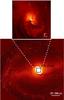 |
Fig. 1 HST F438 wide field image of NGC 1433 from the ESA Hubble Science Archive. The FOV of 10″× 10″ of our SINFONI observations is marked by a square. The color scale in the lower image was chosen to reflect the large scale structure of the host, e.g., the main stellar bar. The top image shows the prominent dust lanes in the center of NGC 1433. |
2. Observation and data reduction
In this paper, we present the results of our ESO SINFONI observations of NGC 1433 with the Unit Telescope 4 of the Very Large Telescope in Chile. The 0.̋25 plate scale was used, which results in an 8″× 8″ field of view (FOV) without adaptive optics assistance. The average seeing was 0.̋5. To increase the FOV and minimize the overlap of dead pixels in critical areas, a ± 2″ dithering sequence was used. Nine dithering positions were used in which the central 4″× 4″ were observed at the full integration time. The resulting FOV is 12 × 12″, but a FOV of 10 × 10″ is used for the analysis. NGC 1433 was observed using the H-band grating with a spectral resolution of R ≈ 3000 and the K-band grating with a resolution of R ≈ 4000. The digital integration time of 150 s was used in both bands with a ...TST... nodding sequence (T: target, S: sky), to increase on-source time. The overall integration time on the target source in H-band was 2400 s and in K-band 4500 s with additional 1200 s in H-band and 2250 s in K-band on sky. The G2V star HIP 017751 was observed in the H- and in K-bands within the respective science target observation. Two object-sky pairs in H-band and four object-sky pairs in K-band were taken. The standard star was used to correct for telluric absorption of the atmosphere and to perform the flux calibration of the target. A high signal-to-noise solar spectrum was used to correct for the black body and intrinsic spectral features of the G2V star (Maiolino et al. 1996). The solar spectrum was convolved with a Gaussian to adapt its resolution to the resolution of the standard star spectrum. The solar spectrum edges had to be interpolated by a black body with a temperature of T = 5800 K. The standard star spectrum was extracted by taking the total of all pixels within the radius of 3 × FWHMPSF, the full width at half maximum of the point spread function (PSF) (Howell 2000), centered on the peak of a two-dimensional Gaussian fit. The flux calibration of the target source was performed during the telluric correction procedure. We calibrated the standard star counts at λ1.662 μm and λ2.159 μm, in H- and K-band, respectively, to the flux given by the 2MASS All-sky Point Source Catalog. A PSF FWHM of 0.̋62 in H-band and 0.̋56 in K-band was measured from the observed standard star (see Fig. 2). The PSF shows an elongation in the northeast to southwest direction at a PA of 69° (see Fig. 3).
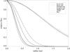 |
Fig. 2 Shown are Gaussian fits to radial luminosity profiles of the K-band standard star continuum, the H-band standard star continuum, the H- and K-bands galaxy continuum, the fitted stellar continuum in the K-band, Fe ii λ1.644 μm, and Brγ. Note that K-band galaxy continuum and the fitted stellar continuum lie on top of each other. The Gaussian fit was centered on the galactic center. |
Detector-specific problems, which occurred during our observation period, were analysed and corrected for and OH sky emission line corrections were applied (see Appendix A).
The data reduction was performed by the SINFONI pipeline up to single-exposure-cube reconstruction. The wavelength calibration had to be refined by hand because of a constant offset introduced to the wavelength axis. The error introduced by this shift is ~3 kms-1. The final cube realignment was done using our own idl routine.
We conducted the investigation and correction of the detector specific problems and the OH lines as well as the linemap and spectra extraction using our own IDL routines.
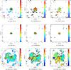 |
Fig. 3 Flux [10-20 W m-2], FWHM [km s-1], and LOSV [km s-1] maps (left to right) of the [Fe ii], Brγ, and H2λ(1−0)S(1) lines (top to bottom). a) and g) show the beam size in the lower left corner for H- and K-band respectively. g) Shows the aperture sizes taken for our measurements. One angular resolution element (beam) corresponds to a PSFFWHM of 0 |
We use calibrated 350 GHz ALMA data to compare with our NIR results (Combes et al. 2013, observation and calibration details therein from the ALMA archive). We used a mask at 50 mJy, 30 mJy and 10 mJy emission level. The map sizes are 720 × 720 pixels with a pixel size of 0 05 for cleaning. The line cube comprises 72 channels of 5 km s-1 width, centered on the systemic velocity, i.e., 1076 ± 180 km s-1. The integrated intensity and continuum maps (line-free regions of all four spectral windows, i.e., 7 GHz) were corrected for primary beam attenuation. Imaging, cleaning, and parts of the analysis have been conducted with the CASA software (v3.3 McMullin et al. 2007).
3. Results
With the seeing limited imaging spectroscopy of VLT SINFONI we resolve the central 500 pc of NGC 1433 at a spatial resolution of 27 pc in K-band and 30 pc in H-band. We identify several molecular ro-vibrational hydrogen lines and the narrow hydrogen recombination line Brγλ2.166 μm. Several stellar absorption features in K-band (e.g., CO(2−0) λ2.29 μm, NaD λ2.207, CaT λ2.266) are detected. The H-band stellar absorption features (e.g., Si i λ 1.59 μm, CO(6−3) λ1.62 μm) and the [Fe ii] λ1.644 μm line, which is important for NIR diagnostics are also detected. The emission lines properties were determined from Gaussian profile fits. A FOV of 10″ × 10″ instead of the available 12″ × 12″ is used because the signal-to-noise ratio (S/N) in our utmost outer regions is not good enough for a thorough analysis.
The new galaxy center is adopted in all figures shown (see Table 1 and Sect. 4.1). The black × in all shown maps gives the position of the new adopted center of the galaxy, i.e., the location of the SMBH. The FWHM maps and values are not corrected for instrumental broadening, which is ~100 km s-1 in H-band and ~75 km s-1 in K-band. Emission line properties, i.e flux and FWHM, of all discussed emission lines are summarized in Table 2.
3.1. Ionized gas
The forbidden line transition [Fe ii] in H-band is detected in a resolved region at the center of about 38 pc in diameter (see Fig. 3). The flux peak is slightly offset by one spaxel (0.̋125) to the south. The shape of the emission looks slightly elongated in the northeast to southwest direction, similar to the PSF elongation. The line-of-sight velocity (LOSV) shows that the line is redshifted with respect to the systemic velocity by ~20 km s-1. The red velocity maximum is ~18 pc south of the center where the velocity is − 45 km s-1. The blue counterpart with a velocity of ~20 km s-1 lies north of the center. The line width is rather uniform with an FWHM of about 185 km s-1 and a faint broadening with an FWHM of 210 km s-1 in the center. The equivalent width (EW) peaks at the same position as the flux with ~2.2 Å indicating that the ionization of the [Fe ii] originates from the very center of the galaxy (see Fig. 5).
Basic data on NGC1433.
Brγ is detected only at the center as well and is marginally resolved in a region with a size of about 30 pc in diameter (see Fig. 3). Only a narrow component of this recombination line can be detected. The emission peaks at the center and is roughly elongated in the eastwest direction. The line width at the very center is with an FWHM ~ 200 km s-1 similar to that of the [Fe ii] emission line but otherwise its at ~150 km s-1 in the emission region. The LOSV shows a blue end in the northwest direction and a red end in the southwest. One might assume a rotation with the line of nodes in this direction (PA ~ 114°), however, the region Brγ is detected in is too small to say much more about the velocity field in the central region. The velocity at the very center is ~30 km s-1 redshifted. The EW is small with a maximum of about 0.8 Å on the nucleus hinting at a nuclear ionization (see Fig. 5).
The line ratio log([Fe ii]/Brγ) can be used to determine the main excitation mechanism (Alonso-Herrero et al. 1997) in the center. In the central emission region with a radius of 1″ a line ratio of 0.8 is measured. This value is rather typical of a mixed ionization by X-ray photons from an AGN (log([Fe ii]/Brγ) ≲ 1.3), stellar thermal UV photons and shocks. If the central Brγ excitation is assumed to be originating from stars only, i.e., no excitation by AGN radiation, the luminosity of Brγ in this region can be used to determine a star formation rate (SFR; Panuzzo et al. 2003; Valencia-S. et al. 2012). We derive an upper limit for the SFR within a 1″ radius around the nucleus of 1.4 × 10⁻³M⊙yr-1 using 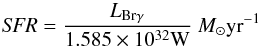 (1)and LBrγ from above. Additionally, if outflows or jets are disregarded as excitation sources in this region and [Fe ii] excitation mainly by shocks from supernovae is assumed an upper limit for the supernova rate (SNR) in the central region can be estimated. Following Bedregal et al. (2009) we use two different estimators
 ![Mathematical equation: \begin{equation} \textit{SNR}_{\mbox{\tiny Cal97}}=5.38\;\frac{L_{[\ion{Fe}{ii}]}}{10^{35}\mbox{W}}\;\mbox{yr}^{-1} \end{equation}](/articles/aa/full_html/2014/07/aa23642-14/aa23642-14-eq56.png) (2)after Calzetti (1997) and
(2)after Calzetti (1997) and ![Mathematical equation: \begin{equation} \textit{SNR}_{\mbox{\tiny AlH03}}=8.08\;\frac{L_{[\ion{Fe}{ii}]}}{10^{35}\mbox{W}}\;\mbox{yr}^{-1} \end{equation}](/articles/aa/full_html/2014/07/aa23642-14/aa23642-14-eq57.png) (3)after Alonso-Herrero et al. (2003). Both authors derive their relation from empirical data analysis. With an [Fe ii] luminosity of L[Fe ii] = 1.92 × 1030 W the SNRs are estimated to be 1.03 × 10⁻⁴ yr-1 and 1.55 × 10⁻⁴ yr-1, respectively. These SFR and SNR values are low (e.g., Rosenberg et al. 2012; Esquej et al. 2014, and references therein) compared to other non-starburst galaxies, particularly with regard to the assumption that all of the central Brγ and [Fe ii] emission is attributed to star formation, which is an unlikely scenario in a Seyfert like galaxy.
(3)after Alonso-Herrero et al. (2003). Both authors derive their relation from empirical data analysis. With an [Fe ii] luminosity of L[Fe ii] = 1.92 × 1030 W the SNRs are estimated to be 1.03 × 10⁻⁴ yr-1 and 1.55 × 10⁻⁴ yr-1, respectively. These SFR and SNR values are low (e.g., Rosenberg et al. 2012; Esquej et al. 2014, and references therein) compared to other non-starburst galaxies, particularly with regard to the assumption that all of the central Brγ and [Fe ii] emission is attributed to star formation, which is an unlikely scenario in a Seyfert like galaxy.
3.2. Molecular gas
At a five sigma confidence level several H2 molecular emission lines are detected: H2(1−0)S(3) λ1.96 μm, H2(1−0)S(2) λ2.03 μm, H2(1−0)S(1) λ2.12 μm, H2(1−0)S(0) λ2.22 μm, H2(2−1)S(1) λ2.25 μm, H2(1−0)Q(1) λ2.41 μm, H2(1−0)Q(3) λ2.42 μm. The most prominent lines are H2(1−0)S(3) and H2(1−0)S(1).
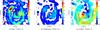 |
Fig. 4 ALMA cycle 0 molecular 12CO(3−2) maps. a) Emission map of 12CO(3−2) [Jy beam-1 km s-1] overlaid with H2(1−0)S(1) emission contours. The red ellipse at −4,4 describes the beam size. The dispersion (moment 2) is shown in b) and the LOSV is shown in c), both maps are in [km s-1]. c) Cuts for the position velocity (PV) diagrams (see Fig. 12). The cuts were not set on the galactic center but along the central velocity gradient of the 12CO(3−2) 1st moment map. |
The line map of H2(1−0)S(1) shows an interesting structure in the nuclear region of NGC 1433 (see Fig. 3g). First, the overall emission follows the dust lanes seen in the HST image (see Fig. 10a). Second, the emission peaks about 0.̋5 northwest offset to the K-band continuum peak and forms an arc-like structure from there toward the southeast, where the continuum peak is located. The LOSV along this region shows a strong gradient from about −40 km s-1 to 40 km s-1. There are also several bright emission spots. The most prominent are two spots 2″− 3″ east-northeast of the nucleus and a less prominent emission region in the west about 2.̋5 away from the center. There are several other emission spots distributed over the spiral dust lanes. The EW map shows that on the continuum peak the EW is ~1 Å while at the H2(1−0)S(1) emission peak it is ~2.1 Å. Moreover, the strongest EWs are seen in the eastern emission spots ranging from about 1.8 Å in the eastern surroundings over 3.4 Å in the northeastern spot (sp(A)) and reaching about 8 Å in the spot (sp(B), see Fig. 5). Emission spot sp(B) shows an FWHM of more than 230 km s-1 and a blue-shifted LOSV of 90 km s-1 whereas the surrounding gas is rather systemic or slightly redshifted. The southern spot sp(B) belongs rather to a spiral arm that is not coupled with the inner nuclear (pseudo-)ring (see Figs. 3, 4) described by Combes et al. (2013). The LOSV is rather blueshifted in the arm west of the center whereas the eastern side is rather systemic (see Fig. 3i). The region south of the nucleus, where the gas is redshifted up to 70 km s-1 in an 1″ distance, indicates a possible outflow. The FWHM in this region is 180 km s-1 whereas in the center it is around 210 km s-1. To the northwest of the nucleus there is a probable blue counterpart at a velocity of only 30 km s-1 and a distance of  . An outflow scenario was thoroughly discussed in Combes et al. (2013). Another possible scenario that can explain this high LOSV gradient in all the emission lines is a gaseous disk in the center of NGC 1433. We will discuss this in Sect. 4.2.
H2(1−0)S(3) is distributed similarly to the H2(1−0)S(1) line. It seems noisier than H2(1−0)S(1) which is due to a spectrally noisier region in which the line is situated. Nevertheless, the line peaks in the same region as H2(1−0)S(1) and has a tail along the K-band continuum peak toward the southeast. Two emission peaks in the east are detected as well as other emission spots that one can identify with bright regions in the H2(1−0)S(1) emission map. The EWs are similar over the whole FOV. The line width shows generally higher velocities than the H2(1−0)S(1) line.
All other detected H2 lines show emission around the center and/or in the northeastern emission spot. The dust lane structure is barely traced in emission line maps other than H2(1−0)S(1) and H2(1−0)S(3).
3.2.1. The H2 mass estimation
The warm H2 gas mass can be estimated following Turner & Ostriker (1977); Scoville et al. (1982); Wolniewicz et al. (1998) as 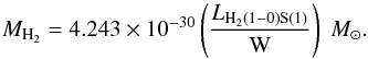 (4)A warm H2 gas mass of 4.89 M⊙ can be estimated at the central 1″ (~54 pc) using an H2 (1−0)S(1) luminosity of LH2(1 − 0)S(1) = 1.15 × 1030 W. Within a 10″ × 10″ FOV a warm H2 gas mass of 19.5 M⊙ is estimated using a 5″ radius aperture centered on the nucleus. The conversion factor determined by Mazzalay et al. (2013) yields
 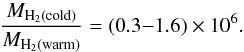 (5)is used to determine the cold H2 gas mass. The cold H2 gas mass of (1.5−7.8) × 106M⊙ is derived for the 1″ radius aperture and (0.6−3.1) × 10
 for the 5″ radius aperture. This means that one third of the H2 in the central 10″ can be found in the central 1″ radius around the nucleus. Combes et al. (2013) derive an H2 gas mass for their outflow, which covers about the same region as our central 1″ radius, of 3.6 × 10⁶M⊙. This is in good agreement with our measurements. However, from our measurements of the 12CO(3−2) emission we estimate an H2 gas mass of 2.1 × 10⁵M⊙ for a 1″ radius and 8.3 × 10⁶M⊙ for a 5″ radius, using the Milky Way dust-to-gas ratio (Solomon & Barrett 1991).
3.3. Continuum
To address the continuum emission in the nuclear region of NGC 1433 a decomposition as described in Smajić et al. (2012) was used. The continuum shows only a stellar contribution with almost no extinction needed for the fit. Hence, the K-band continuum and the stellar continuum peak in the same position and their photon distributions look very similar. The stellar continuum was obtained by fitting the CO(2−0) bandhead with a stellar spectrum. Stellar templates from Winge et al. (2009) were used as input for the fitting routine. The template spectra were convolved with a Gaussian to adapt the resolution to our SINFONI resolution of 4000 in K-band. The red giant HD2490 – spectral class M0III – fitted best without the need of additional stellar spectra (e.g., asymptotic giant branch stars). What might be surprising is the fact that the NIR continuum peak coincides with the optical, HST images from F450W, F660W, and F810W filters, and is not affected by the obvious dust lanes seen in Fig. 10a. Unfortunately, the spectra of these template stars have a wavelength coverage of only 2.2 μm to 2.4 μm. Therefore, the fitted spectral region is small, which may explain why no extinction component was needed for the fit, even at the spatial positions of the dust lanes.
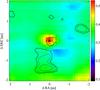 |
Fig. 6 H − K color diagram in magnitudes showing the center of NGC 1433 measured in the SINFONI H- and K-band. The contours are from the 0.87 mm continuum emission measured by ALMA. For detail, see Sects. 3.3 and 4.1. |
The H − K color map (see Fig. 6) shows no reddening at the dust lane position, but toward the newly adopted center a strong reddening in H − K is detected. This can be taken as a signature of hot dust at the sublimation temperature. In AGN, this hot dust is located at the sublimation radius, which is co-spatial with the outer edges of the accretion disk and/or the inner edge of the circum-nuclear torus. From the CO(2−0) band head fitting the LOSV of the stars can be determined and a rotation direction at a PA ~ 201° is measured. The velocity field seems to be systematically redshifted by a few km s-1. A reason may be the imperfect wavelength calibration as stated in Sect. 2. The projected velocities range from about −50 to 60 km s-1 and the 0 km s-1 isovelocity contour lies close to the continuum center. The line-of-sight velocity dispersion (LOSVD) ranges from about 90 to 160 km s-1. From the velocity dispersion we can determine a black hole mass, assuming that NGC 1433 lies on the M-σ relation. Following Gültekin et al. (2009),  (6)we determine a black hole mass of M• = 7 × 10⁶M⊙ with an assumed velocity dispersion of σ∗ = 100 km s-1, which is measured at the very center where a minimum in LOSV is measured. A minimum in the LOSVD is often found in galaxies with a nuclear disk that is not always resolved (Emsellem et al. 2001; Falcón-Barroso et al. 2006). By assuming a Gaussian distribution of the fitted LOSVD over our FOV (see Fig. 7), we determine a mean velocity dispersion of 125 ± 10 kms-1 hence, a black hole mass of M• = (1.8 ± 0.8) × 107M⊙. The first estimate agrees with Buta (1986), however, the latter represents the bulges LOSVD, which is needed for the equation given above.
From the shape and angle of the K-band continuum isophotal ellipses we deduce that the PA of the nuclear stellar oval or bar is ~ 33° (see Fig. 8b, 9c). For the isophotal lines that range from 25% to 35% of the peak luminosity the PA changes to 15° before it shifts to a PA of about 70° for the inner isophotes. The change in angle toward the inner isophotal lines can be attributed to the PSF, which is as well elongated in the northeast to southwest direction at a PA of ~70°.
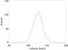 |
Fig. 7 The fit over the stellar dispersion from the continuum decomposition in 5 kms-1 bins. The X-axis shows the fitted dispersion and the Y-axis the total number of spatial pixels that corresponds to this dispersion bin. The red curve represents a Gaussian fit to the distribution. |
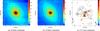 |
Fig. 8 From left to right H-band, K-band [10-18 W m-2μm-1], and 0.87 mm [Jy beam-1] continuum. c) H2(1−0)S(1) contour overlaid on the 3 sigma clipped 0.87 mm continuum. For details, see Sects. 3.3 and 4.1. |
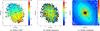 |
Fig. 9 a) Fitted stellar LOSV map [km s-1], b) stellar disperion [km s-1], and c) stellar continuum (arbitrary unit) map. In panel a) the LOSV PA of the galactic rotation is marked. Panel c) shows probable PAs of the isophotes where the largest cross marks the PA of the nuclear bar and the smallest cross the orientation of the beam. The middle cross indicates a possible twist in the isophotal lines. |
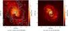 |
Fig. 10 a) An HST map at about 4380 Å with H2(1−0)S(1) contours overlaid. b) Same HST image in the ALMA FOV with the 12CO(3−2) line emission in contours. The HST images were taken from the archive and were observed with the WFC3 instrument and the UVIS detector using the F438W filter. The images illustrate the remarkable overlap of dust lanes and molecular hydrogen a) and 12CO(3−2) emission b), respectively. |
 |
Fig. 11 Stellar LOSV subtracted maps of H2(1−0)S(1) and 12CO(3−2). c) is the same as b) but 20 km s-1 were added to the residual to indicate the higher resemblance with panel a). All color-bar units are in km s-1. For details, see Sect. 4.2. |
Emission lines.
4. Discussion
4.1. The nucleus of NGC 1433
One result from the continuum decomposition (see Sect. 3.3) is that the NIR stellar peak at the center does not fall onto the 0.87 mm continuum peak measured with ALMA (see Fig. 8c). To address this issue the H2(1−0)S(1) contours were overlaid on the HST F450W map, the ALMA 12CO(3−2) map, and the 0.87 mm continuum map (see Figs. 4a, 8c, 10a). In Fig. 10a the dust lanes are well covered by the H2(1−0)S(1) emission when the stellar NIR peak (marked with an ×) is placed onto the brightest pixel in the HST image. Furthermore, the H2(1−0)S(1) emission contours were overlaid on the ALMA 12CO(3−2) map (see Fig. 4a). The molecular CO emission fits best to the molecular H2 emission when the stellar continuum center is placed on a small local CO peak about 1.̋5 north and 0.̋2 west from the assumed center in Combes et al. (2013). Finally, the H2(1−0)S(1) contours were overlaid on the 0.87 mm continuum map by aligning it to the same spatial pixel that was found from the overlay onto the 12CO(3−2) map (see Fig. 8c). Interestingly, the NIR stellar continuum peak is situated on a local 0.87 mm peak that is about three-quarters as strong as the brightest 0.87 mm peak. The eastern side of the central arclike structure in the H2(1−0)S(1) line map as described in section 3.2 traces a 0.87 mm emission toward the peak of the 0.87 mm emission. Furthermore, the H − K color diagram in Fig. 6 shows that toward our adopted center the color becomes significantly redder, resulting from the warm dust emission of the SMBH surrounding torus. Unfortunately, the bright spots in the 12CO(3−2) and the H2(1−0)S(1) emission maps, which could be used to align the NIR and the submillimeter maps, do not coincide exactly with each other.
As shown in Fig. 4a, the brightest 12CO(3−2) region, in the northeast, is very well traced by the H2(1−0)S(1), as well as the bright clumps in the west. A proper alignment can be obtained using these emission regions as it is also appreciable in the correspondence of the extended flux of both emitting species. The error estimate of the center positioning, using the described method, turns out to be 02. The estimated error becomes evident when studying the 0th and 1st moment maps of 12CO(3−2), overlaid with the corresponding H2 maps. The error represents a shift of the ALMA data with respect to our NIR/optical center. By shifting the CO maps with respect to the H2 emission line map a cross-correlation of the strongest 12CO(3−2) emission spots with probable corresponding emission in the H2 map is performed. Additional support for the newly estimated nuclear position is the strong velocity gradient across this region in all emission lines, e.g., 12CO(3−2), H2(1−0)S(1), Brγ, and [Fe ii]. Also, [Fe ii] and Brγ only show detectable emission at the position of the stellar continuum peak co-spatial with emission from the circum-nuclear hot dust. The exact position of the adopted new center is given in Table 1. This is convincing combined evidence for the presence of an AGN and a SMBH at the newly found position.
4.2. The central arcsecond
As already mentioned in Sect. 3.2 the high velocities in the central region were already discussed for the 12CO(3−2) line observed with ALMA. Combes et al. (2013) argued mainly about an outflow scenario and its origin. Although they placed the center of NGC 1433 and therefore the AGN more than 1″ further south, their argument is still solid. But, because of the change in the position of the center a rotating gaseous disk surrounding the nucleus and the center of the stellar distribution of NGC 1433 needs to be considered an alternative solution.
A central nuclear disk? In H2 a velocity gradient of −40 km s-1 to 40 km s-1 is measured at a 1″ diameter distance over the nucleus (see Fig. 3i). This gradient is higher in 12CO(3−2) reaching velocities of −80 km s-1 to 120 km s-1 (see Figs. 4c,12a). Using the H2(1−0)S(1) velocities we determine a central mass to be Mcent of 7.3 × 10⁶M⊙. This mass is in-between the two measured black hole masses determined using the M–σ elation (7 × 10⁶ and 1.7 × 10⁷M⊙, see also Sect. 3.3). The velocity gradient across the center is at a PA of 140° and is aligned with the farside of the galaxy whereas the stellar velocity gradient is at a PA of 201°. This nuclear velocity gradient is seen in all detected NIR emission lines except for [Fe ii], which can also resemble a north-south aligned gradient.
There is a discrepancy in the line of nodes angle between H2 and 12CO(3−2). For 12CO(3−2) we measure a line of nodes PA of 155°, this difference is visible in the LOSV maps of the respective lines (see Figs. 3i,4c). The effect is probably introduced by PSF smearing since we are looking at a barely resolved region. A possible inclination (face-on to edge-on) of this gaseous nuclear disk cannot be determined from this data and since the PA differs strongly from the stellar PA a rotation in the galactic disk plane does not distinguish itself.
The position–velocity (PV) diagram in Fig. 12a shows a possible central rotating disk profile that reaches the maximum velocities of ±100 km s-1 at  from the center. Here the PA of the PV diagram was chosen based on the velocity field in the central region (see Fig. 4c). Assuming an edge-on disk, a lower limit for the dynamical mass is estimated to be 4 × 10⁷M⊙ with the measured velocity and radius. This mass is higher than our estimated BH mass values. However, we derived here the dynamical mass within an aperture of
  radius, which is supposed to be higher than the BH mass since it accounts for the stellar mass included in this aperture. Assuming that the inclination is i = 33° this implies a higher mass by a factor of 3 (see Combes et al. 2013). But inclination and PA of a circum-nuclear disk do not at all have to agree with the corresponding values of the larger scale galaxy structure. A large stellar mass contribution for the inner 20 pc can be expected for NGC 1433. For example, at the center of the Milky Way, the mass density in the inner parsec reaches values of the order of 105M⊙ pc-3 (see Fig. 22 by Schödel et al. 2009, 2002). This results in an enclosed stellar mass of 4 × 10⁷M⊙ pc-3 at a radius of 10 pc and about 108M⊙ pc-3 at a radius of 20 pc. This implies also that in the case of NGC1433, the stellar mass contribution will be substantial.
The tips of the disk are located at the slightly increased dispersion spots as seen in the 2nd moment 12CO(3−2) image (Fig. 4b). The lack of 12CO(3−2) emission at the very center can be explained by highly excited (possibly even optically thin) molecular gas at temperatures of >55 K, which is suppressed in its emission through the 12CO(3−2) transition. Molecular rings filled in by line emission of higher rotational transitions are a commonly observed phenomenon in galactic nuclear regions. In the case of I Zw 1, Staguhn et al. (2001); Eckart et al. (2001, 2000) have shown that the circum-nuclear ring structure, which is present in interferometric 12CO(1−0) maps, is not evident in 12CO(2−1) maps since the center of the ring has been filled up by 12CO(2−1) line emission enhanced through higher molecular excitation toward the nucleus. There is also ample evidence of elevated 12CO(3−2)/(1−0) ratios toward the central positions of galactic nuclei, as demonstrated by Irwin et al. (2011). Their Fig.7 shows that at densities of 104 cm-3 a variation of that ratio by a factor of up to 4 can be obtained if the molecular gas temperature varies between typical nuclear (Muraoka et al. 2007; Tilanus et al. 1991; Israel et al. 2006) and off-nuclear values (Mauersberger et al. 1999; Wilson et al. 2009) of T ~ 50 K and T ~ 10 K. A behavior of the molecular gas structure around an AGN such as this is also expected theoretically, based on three-dimensional non-LTE calculations of CO lines (Wada & Tomisaka 2005).
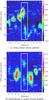 |
Fig. 12 PV diagrams from the 12CO(3−2) ALMA cube a) along the central velocity gradient (PA = 140°) and b) perpendicular to the central velocity gradient (PA = 50°). The color-bar shows the flux density in [Jy beam-1]. The position of the cuts is displayed in Fig. 4c. The white rectangle marks the nuclear region in which the central velocity gradient is dominant. (a1) to (b3) mark dust arm positions: (a1) eastern arm, (a2) southern arm, (a3) nuclear arm, (a4) northern arm, (b1) overlap between eastern and southern arm, (b2) nuclear arm, (b3) southern arm (west). |
The H2 mass derived in the nuclear region is an indicator that the gas close to the nucleus is indeed highly excited since we derive a lower mass from the 12CO(3−2) transition than from the H2(1−0)S(1) transition. To resolve this issue, however, we need submm observations of the central region at higher frequencies and higher angular resolution.
The central nuclear outflow: the newly determined nuclear position agrees well with the kinematic origin of a potential molecular outflow. Interpreting the observed nuclear [Fe ii] and Brγ line emission as tracers of star formation activity (see Sect. 3.1) make star formation an unattractive source for driving such an outflow. In fact, it is very likely that intermittent nuclear accretion events are the driving force (see also Combes et al. 2013).
The rotation profile might as well be produced by an outflow, which is then smeared out by the PSF to look like a rotation. We estimate the disk radius to be about 04, by measuring the distance of the absolute disk velocity maxima from the center, which is about the size of the PSF. The PV diagram perpendicular to the velocity gradient (see Fig. 12b) shows conspicious faint emission lobes at the 0″ position and at a velocity of about ± 60 km s-1. Almost no emission is detected in-between these velocities on the nucleus, which is expected for a molecular disk, but not necessary (see above). The other emission lobes in the PV diagram are the molecular arms.
A combined model: a third possibility is a combination of rotating disk and outflow. This scenario would explain the rotational character of the center and the red tail south of the nucleus visible in H2(1−0)S(1) and 12CO(3−2). Assuming a disk with a single sided outflow away from the observer this also explains the higher redshifted velocity compared to the blueshifted velocity in the SINFONI observation. The different PAs of the central velocity gradients as measured for H2 and CO might then be introduced by PSF smearing due to the higher 12CO(3−2) velocity of the outflow compared to the H2 velocities. This approach confirms the increased redshifted velocity 1″ south of the nucleus seen in the H2 and CO LOSV images (Figs. 3i, 4c) that follow the 0.87 mm continuum tail.
Due to the newly determined position of the center of NGC1433 the outflow’s origin is the SMBH, located at the connection point of blueshifted and redshifted gas in the center. With the new central position we can now also explain the off-nuclear dust continuum emission. Figure 8c shows the 0.87 mm emission overlaid with H2(1−0)S(1) emission contours. Comparing these two emission maps shows that radio continuum emission is present at least at the center and with its emission peak about 15 south of it. Following the H2(1−0)S(1) emission from nucleus to radio continuum peak one traces also weak radio continuum emission. This emission is a three sigma detection and the overlap of radio continuum and H2 emission is remarkable. This radio continuum trail puts the outflow(+disk) scenario at least in front of the rotational disk only scenario. The trail is then explained by gray body dust emission where the dust was excited by the outflow. Interestingly, the EW of H2(1−0)S(1) is almost constant along this trail and around the nucleus except for the emission peak. One might expect an increase of the EW in the outflow regions with respect to the surroundings because of higher H2 fluxes, but none can be detected in any of the emission lines. The dust lane 2″ south of the nucleus shows the same EW as the outflow tail region.
4.2.1. A simple model approach
To substantiate the discussion, three simple models for the central velocity gradients were derived. A disk model based on a differentially rotating edge-on disk with a rotational velocity of v ~ 100 km s-1 at the outer edge was constructed (see Fig. 13a). An inclination parameter was not taken into account since this would mainly change the value of the LOSV of the disk. For the outflow model a constant velocity of v ~ 100 km s-1 was assumed up to a radius of  (see Fig. 13b). A fixed inclination of 30° was chosen for the outflow. The orientation for both models is at a PA of 130°. The scale height (e.g., disk thickness and width of the outflow) was chosen to be 3 spatial pixels. A change in scale height results directly in a different observed LOSV, therefore, this parameter was fixed as well. These two models were then convolved with a Gaussian PSF, using the FWHM measurements of the telluric standard star in K-band. These models were placed on an emissionless background.
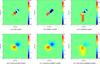 |
Fig. 13 Models used in Sect. 4.2.1 are presented: a)−b) are the constructed models, d)−f) are the PSF convolved models. For details, see Sect. 4.2.1. |
As a result, the convolved models of disk and outflow look very similar and cannot unambiguously be traced back to their underlying model. The models fit well in the central 1″ diameter region. The redshifted part, however, shows an elongated tail southward, which cannot be accounted for with these two isolated models.
Therefore, we chose as a third model a combination of the disk model as described above and a one-sided outflow model. The outflow is now at a PA of ~175° and only the redshifted part is taken into account. The radius of the disk is the same as above. The radius for the outflow is  . The velocities chosen for this model are 60 km s-1 for the disk and 80 kms-1 for the outflow. The convolution was done with the same PSF as mentioned above. The combined model is shown in Fig. 13c. To derive similar velocities as in our H2(1−0)S(1) LOSV map, we changed the velocities of disk and outflow and the PA of the outflow only. All other parameters have the same values as described above. A one-sided outflow can be justified if an otherwise double-sided nuclear wind makes contact with a molecular cloud on only one side.
This third approach can describe the central gradient and the southward going redshifted tail. Figure 14 shows a 4″ × 4″ detail of the H2(1−0)S(1) velocity field centered on the nucleus and the model subtracted residual. The residual is at 0 ± 10 kms-1 in the vicinity of the central gradient. The redshifted tail shows higher redshifted residuals at ~1″ distance from the center, which can mainly be attributed to the underlying galactic rotation.
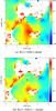 |
Fig. 14 a) Shows the central 4″ × 4″. b) Shows the same detail but subtracted by the combined model (see Fig. 13f). For details, see Sect. 4.2.1. |
4.3. The dusty nuclear spiral arms
The primary bar of NGC 1433 has an efficient way to pull gas toward the central region where it accumulates in a nuclear ring of about 10″ radius (see Fig. 1). This is where the nuclear star formation ring gathers its fuel from – note the various bright spots (probably stellar clusters) in Fig. 10b. From this nuclear ring several dust lanes wind toward the center forming a pseudo-ring of about 4″ radius right outside the inner ILR (iILR) at 36 Buta et al. (2001). The dust arms show differential LOSV patterns as seen in Figs. 3i and 4c.
In the 10″ × 10″ FOV we identify at least three different arms. The northern arm comes from the north along the western side toward the center and is blueshifted. The southern arm stretches from the west along the south toward the emission peak in 12CO(3−2) and is rather redshifted. The eastern arm comes from the south out of the 10″ × 10″ FOV and also goes toward the 12CO(3−2) emission peak but is blueshifted (see Fig. 4c). The western part of the inner 2″ is quite blueshifted and seems connected to the region of the H2 nuclear peak. This nuclear arm also extends southward and turns around from the south to the north toward the nucleus and becomes more redshifted the closer it gets.
The arms are well detected in 12CO(3−2) and the LOSVs are similar to the H2 LOSVs except in one region that belongs to the eastern arm. This H2(1−0)S(1) emission, sp(B) (see Sect. 3.2), is the most blueshifted region in the H2 LOSV map. It reaches almost –100 km s-1 at a distance of 35 to the nucleus. In the region north of it, sp(A) (see Sect. 3.2), the strongest 12CO(3−2) emission does not seem to be as blue as the eastern arm or as red as the southern arm, but rather a mix of both. This region is where, eastern and southern arm meet or overlap, which would explain the strong 12CO(3−2) and the H2 emission there. Note that although we see a maximum in 12CO(3−2) emission the dust lane here becomes fainter as seen in the HST images. The southern spot sp(B) is stronger in H2 than sp(A) and shows an FWHM of up to 250 km s-1. Either we see an interaction between the two arms already or we see a massive star formation region hidden behind and pushing at all the dust and gas. At least this would explain the strong blueshift and the strong H2 emission due to UV excitation. The linewidth of the H2 line in sp(B) speaks in favor of a collision of the two arms. Also, no Brγ emission can be detected in sp(B), which would imply that the column density of the dust and molecular gas (e.g, H2) between observer and star forming region has to be very high so that the H ii region cannot be detected. In addition, no CO emission peak coincides with the position of sp(B). The velocity dispersion in the arms at 2″ distance from the nucleus is up to 50 km s-1 and higher (see Fig. 12), which may indicate an arm–arm interaction or hidden star formation activity.
The measurements of the stellar LOSV with an PA of 21° are consistent with measurements by Buta et al. (2001). The stellar continuum map shows an angle of 33° for the nuclear bar, which is confirmed by Combes et al. (2013). There does not seem to be a greater disturbance in the stellar distribution. A minor twist from 33° in the outer isophotes to 15° and then to 69° toward the central isophotes is detected (see Fig. 8). The central isophotes are dominated by the PSF structure, which is also elongated along a PA of 69°. An ellipses fit to the continuum in optical and NIR confirms our PA measurements.
4.4. Computation of the torques
A nuclear bar is well detected in NIR images of NGC 1433 (see, for example, Jungwiert et al. 1997). It lies inside the nuclear ring, and extends out to about 400 pc in radius, with a position angle of PA = 30°. Inside the ring, a patchy nuclear spiral structure was discovered in HST images by Peeples & Martini (2006). In the present HST data set the dust extinction is smallest in the I-band image that we select to trace the old stellar component, and derive the gravitational potential with high spatial resolution. We have not separated the bulge from the disk contribution, considering that the bulge is highly flattened. Buta et al. (2001) concludes, on the basis of both photometry and kinematic arguments, that the inner part of the bulge is as highly flattened as the disk. The dark matter fraction is also negligible in the central kpc. The HST-F814W image has been rotated and deprojected according to PA = 19° (equivalent to 199°) and i = 33°, and then Fourier transformed to compute the gravitational potential and forces. A stellar exponential disk thickness of ~1/12th of the radial scale-length of the galaxy (hr = 3.9 kpc) has been assumed, giving hz = 328 pc. This is the average scale ratio for galaxies of this type (e.g.„ Barteldrees & Dettmar 1994; Bizyaev & Mitronova 2002, 2009). The potential has been obtained assuming a constant mass-to-light ratio of M/L = 0.5M⊙/L⊙ in the I-band over the considered portion of the image of 2 kpc in size. This value is realistic in view of what is found statistically for spiral galaxies (Bell & de Jong 2001). The pixel size of the map is 0.1′′ = 4.8 pc. The stellar M/L value was fit to reproduce the observed CO rotation curve.
The potential was decomposed into its different Fourier components, as in Combes et al. (2014). The radial distribution of their normalized amplitudes and their radial phase variations are displayed in Fig. 15.
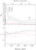 |
Fig. 15 Top: strengths (Qm and total QT) of the m = 1 to m = 4 Fourier components of the stellar potential within the central kpc. Inside a radius of 130 pc, the m = 1 term dominates, and the nuclear bar extends until 350 pc radius. Bottom: corresponding phases in radians of the Fourier components, taken from the major axis, in the deprojected image. |
From the potential, we derive the torques at each pixel, as described in García-Burillo et al. (2005). The sign of the torque is determined relative to the sense of rotation in the plane of the galaxy. The product of the torque by the gas density Σ is shown in Fig. 16.
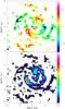 |
Fig. 16 Top: map of the gravitational torque, t(x,y) × Σ(x,y), weighted by the gas surface density Σ, assumed proportional to the 12CO(3−2) emission. The torque per unit mass is t(x,y) = xFy − yFx at each pixel (x, y), where Fx and Fy are the forces per unit mass, derived from the potential. The torques change sign as expected in a four-quadrant pattern (or butterfly diagram). The orientation of the quadrants follows the nuclear bar’s orientation. In this deprojected picture, the major axis of the galaxy is oriented parallel to the horizontal axis. The inclined line reproduces the mean orientation of the bar (PA = 101° on the deprojected image). Bottom: deprojected image of the 12CO(3−2) emission, at the same scale, and with the same orientation, for comparison. The axes are labeled in arcseconds relative to the center. The color scales are linear, in arbitrary units. |
The torque weighted by the gas density Σ(x,y) is then averaged over azimuth, and allows us to estimate the time variations of the specific angular momentum L of the gas. The torque efficiency in driving gas flows is then obtained by normalizing at each radius by the angular momentum and rotation period, as shown in Fig. 17.
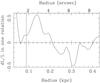 |
Fig. 17 Radial distribution of the torque, quantified by the fraction of the angular momentum transferred from the gas in one rotation, dL/L, estimated from the 12CO(3−2) deprojected map. The vertical line at 88 pc radius delimits the extent of the central gas outflow, and the computation has no meaning here. The torque is positive inside a 200 pc radius and then negative outside. |
The definition of the exact center of the galaxy has an uncertainty of ±0.2 arcsec. To estimate the implied uncertainty on the torques, we have computed them with several centers, displaced by ±0.2 arsec in RA and DEC. This resulted in an uncertainty of about 20% on torques.
Although the nuclear bar strength is diluted by the flattened bulge, Fig. 17 shows that its efficiency is still high. Between 88 and 200 pc, the gas gains up to 50% of its angular momentum in one rotation, i.e., in ~40 Myr. Outside of this radius, the torque is negative. The radius of 200 pc corresponds to a pseudo-ring, which Combes et al. (2013) interpreted as the inner ILR of the bar, i.e., the ILR of the nuclear bar. The observed torques drive the gas toward this ring, and re-inforce it. Inside 88 pc, the torque results have no meaning, since we observe mostly outflowing gas, dragged by the putative AGN jets (Combes et al. 2013). The computation cannot be interpreted in terms of average torque here, since the gas is not in quasi-stationary orbits in rotation around the center of the galaxy, aligned on the galaxy plane. Instead, the gas is ejected at some angle from the plane (Combes et al. 2013), and the deprojections and torque computations do not apply here.
In summary, the gravity torques appear negative at a radius of R> 200 pc and positive at R< 200 pc. This leads to a accumulation of gas at the position of the R = 200 pc ring, which is expected for the ILR of the nuclear bar. To drive the gas further in, other mechanisms, such as viscous torques or dynamical friction, have to be invoked to take over and fuel the nucleus.
4.5. Line diagnostics
The nuclear region and emission spots sp(A) and sp(B) are the only regions to show a variety of line species that allow for a line diagnostic. The diagnostic diagram of the logarithmic line ratios of H2(1−0)S(1) over Brγ and [Fe ii] over Paβ distinguishes three different galaxy types. Starburst galaxies, in the lower left of Fig. 18, are photoionized and show very high H ii emission. The LINERs are mainly shock ionized, hence shock tracers like H2(1−0)S(1) and [Fe ii] λλ 1.257 μm, 1.644μm show stronger emission. Since both excitation mechanisms can be found in Seyfert galaxies this galaxy type is placed between the two extrema.
NGC 1433 takes its place in the AGN regime (see Fig. 18), but it is close to the shock ionized LINERs. Aperture effects might shift the classification into the LINER regime. This is mainly due to a deficiency of H ii in the central region where we detect Brγ only in the very center, the location of the nucleus. We confirm earlier classifications (e.g., Véron-Cetty & Véron 1986; Cid Fernandes et al. 1998) that describe this galaxy as being Seyfert and LINER like. Because of the borderline classification of NGC 1433 as being a Seyfert/LINER galaxy, scenarios that include outflows are further supported.
The conversion between the [Fe ii] λ1.644 μm flux, obtained from our H-band observation and [Fe ii] λ1.257μm was done using the factor λ1.644 μm/λ1.257 μm = 0.744 (Nussbaumer & Storey 1988). For the conversion of Brγ to Paβ the case B ratio of Brγ/Paβ = 0.17 was used, for a temperature of T = 104 K and an electron density of ne = 104.
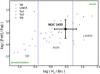 |
Fig. 18 Diagnostic diagram to classify the emission at the nucleus. The [Fe ii] λ1.257 μm and Paβ values were derived from the [Fe ii] λ1.644 μm and the Brγ line. |
The detection of several molecular hydrogen emission lines allows for a line ratio diagnostic (Rodríguez-Ardila et al. 2005). There are three main excitation mechanisms of molecular hydrogen in the NIR, namely: (i) UV fluorescence (non-thermal); (ii) X-ray heating (thermal); and (iii) shocks (thermal).
(i): UV-fluorescence: highly energetic UV photons from theLyman-Werner band (912−1108 Å) are absorbed byH2 molecules and then reemitted at lowerfrequencies. This can occur in a warm high-density gas whereone finds thermal emission line ratios for the lower levels.Because of the high density, the lower levels are dominated bycollisional excitation. Hence, observations of the higher leveltransitions are required to distinguish UV pumping(non-thermal) from collisional excitation (thermal).
(ii): X-ray heating: X-ray dominated regions in which H2 is mainly ionized by X-rays are observable in regions with temperatures <1000 K. At higher temperatures, shock excitation due to collisions populates the lower excitation levels. The ionization rate per H-atom is limited to <10-15 cm3 s-1 since higher rates will destroy the H2 molecules (e.g., Tine et al. 1997; Draine & Woods 1990; Maloney et al. 1996). In dense, static photodissociation regions UV instead of X-ray photons can heat the molecular gas.
(iii): Shock fronts: the collisional thermal excitation via shock fronts in a medium populates the electronic ground levels of H2 molecules. This population of the ro-vibrational transitions is described by a Boltzmann distribution. The kinetic temperatures in these shock excited regions can be higher than 2000 K (Draine & McKee 1993).
Non-thermal excitation cannot be the excitation mechanism in any of our analysed regions since all regions show (2−1)S(1)/(1−0)S(1) ratios of <0.2 (see Fig. 19). The central region is situated above the thermal emission curve, which is probably due to an overestimation of the (1−0)S(3) line that is situated in a noisy spectral region. Nevertheless, Rodríguez-Ardila et al. (2005) show that the bulk of Seyfert galaxies, independent of Seyfert type, have similar or even higher (1−0)S(3)/(1−0)S(1) ratios than our nuclear region. Hence, thermal excitation is the dominant mechanism in the center but further differentiation cannot be concluded.Emission spot sp(A) lies on the thermal emission curve at an excitation temperature between 2000 K and 3000 K. This implies that the gas there is heated up, probably by a hidden star formation region. The 12CO(3−2) map shows the brightest emission in this region. The star formation region has already formed stars by then, which explains that Combes et al. (2013) report a nondetection of the dense gas tracers HCO+(4−3) and HCN(4−3) in this region. The fact that we do not detect Brγ emission hints at a high column density toward the star forming region’s H ii region.
Emission spot sp(B) lies slightly off the thermal excitation curve at about 2000 K and is close to the predicted shock excitation models by Brand et al. (1989). The 12CO(3−2) shows no increased flux in this region hence sp(B) seems not to be excited by the same mechanisms as sp(A). The broadness of the H2 lines in sp(B) as well as the very blueshifted velocities indicate an interaction of the two arms, eastern and southern arm (see Fig. 4c). Due to the interaction of the arms shock fronts are induced in the gas, which then excite the H2 molecules in sp(B). Another possibility is a strong star formation that shocks the surrounding gas. As in sp(A) no Brγ or HCO+(4−3) and HCN(4−3) are detected indicating either a high column density toward the region, a not strong enough ionization source or not dense enough gas.
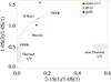 |
Fig. 19 Molecular hydrogen diagnostic diagram to classify the emission at the nucleus in red and in emission spots sp(A) in green and sp(B) in blue. Line ratios are H2(2−1)S(1)/H2(1−0)S(1) and H2(1−0)S(3)/H2(1−0)S(1). The curve represents thermal emission at 1000–3000 K. Horizontal stripes are thermal UV excitation models by Sternberg & Dalgarno (1989). Vertical stripes are non-thermal models by Black & van Dishoeck (1987). The area of X-ray heating models by Draine & Woods (1990) is marked by an open triangle (yellow). The open turquoise circle marks the region of the shock model by Brand et al. (1989). |
5. Conclusion and summary
We have presented the first ALMA backed SINFONI results for the nearby LINER/Seyfert 2 galaxy NGC 1433 from the extended NUGA south sample. We constrain the center of the galaxy and the black hole position to the optical and NIR stellar luminosity peaks with an error of ±02. The new center lies about 15 north-northwest from the adopted center (see Table 1) by Combes et al. (2013).
With the new adopted center, we discuss the velocity field of the H2 and CO gas in the very center and propose three interpretations of the results: gaseous disk, molecular outflow, or a combination of both. No outflow characteristics were observed in X-ray, however, the 2″ resolution is insufficient to trace the possible outflow that we describe above. Our simple modeling approach shows that, spatially, there is no difference between a central disk model and a nuclear double-sided outflow. Depending on the yet unknown inclination the disk might be decoupled. Furthermore, the combination of a circum-nuclear disk and a one-sided outflow is a scenario that can explain the southward reaching redshifted tail as well as the central velocity field, but it has a higher number of degrees of freedom.
Further analysis of the spiral arms and their LOSVs hints at an inflow scenario for the center of NGC 1433 (see Fig. 11). The dust arms seem to leave the disk, which is implied by the blue LOSV 2″ west of the nucleus and turn around again to fall in the direction of the nucleus where they encounter the strong nuclear velocity gradient that is oriented at a PA ~ 140°. Our torque calculations show that the gas is driven toward a nuclear ring of 200 pc radius, which could be the ILR of the nuclear R = 430 pc bar. A possible gas infall toward the very center requires that other mechanisms, e.g., viscous torques, can take over from there. Indeed, we see several dust arms within a 2″ radius, i.e., the nuclear-arm and several faint dust lanes (see Fig. 10) that could be driven inward by viscosity torques (Combes et al. 2004; van der Laan et al. 2011). The observed dip in LOSVD of the stars can then be explained by infalling gas that creates a nuclear disk in which stars are formed with a lower velocity dispersion than the bulge LOSVD (Emsellem et al. 2001; Falcón-Barroso et al. 2006).
The PV diagrams speak in favor of an outflow (see Fig. 12) scenario. With the new center, the outflow has its origin at the position of the SMBH. The lower H2 velocity with respect to the CO velocity in the nuclear region indicates a shock ionization of the gas. However, a small circum-nuclear disk cannot be excluded.
The measurement of the stellar LOSV is consistent with literature values. The isophotes in the central region follow the nuclear bar structure although a small deviation may be detected toward the center (see Fig. 9).
The emission lines allow a line diagnostic on the nucleus and in emission spots sp(A) and sp(B). We confirm a Seyfert-to-LINER like excitation mechanism from the diagnostic diagram in Fig. 18. An outflow inferred from strong star formation in the center can be excluded because of a very low SFR. Thermal excitation dominates emission spots sp(A) and sp(B). The thermal emission temperature is higher in sp(A) than in sp(B) whereas sp(B) is close to the shock excitation models by Draine & McKee (1993). Spot sp(A) lies exactly on the thermal emission curve at ~2500 K. We detect either hidden star formation in sp(A) and sp(B) or a strong dust arm interaction in sp(B) due to strong 12CO(3–2) and H2 emission in sp(A) and strong and turbulent H2 emission in sp(B).
We measure a stellar mean LOSVD of 124 km s-1 and determine a black hole mass of M• = 1.74 × 10⁷M⊙, which is higher than literature values by a factor 2. The H2 gas mass is derived from 12CO(3−2) and from the warm H2 gas in the NIR. We derive in the central 1″ radius aperture an H2 mass of ~106M⊙ from the warm NIR gas, which is a factor 2 higher than the value from the CO luminosity. We derive from both lines a mass of ~107M⊙ for the larger central 5″ radius aperture. This difference in the center may result from a lack of emission of the 12CO(3−2) transition due to highly excited gas with temperatures of >55 K.
The dust and gas arms reach toward the center. But is the center accreting this gas mass through a disk? Or is it repelling a possible infall through an outflow? Or do we see both mechanisms working without any larger interaction? Higher spatial resolution in forthcoming ALMA cycles and SINFONI with AO assistance as well as higher excited CO transitions are needed to sufficiently resolve the center and the mechanisms that create this strong gradient that is not aligned with the stellar rotation.
Online material
Appendix A: Detector-specific pattern and atmospheric emission correction
During the data reduction we had to address a problem with the SINFONI detector that occurred during the observing period. The detector amplifiers introduce two different types of variation in the arbitrary digital units (ADU) (see Fig. A.1). These variations would come and go from exposure to exposure and were also found in the calibration data provided to the observation data. From our investigation of the affected files we have recognized this problem in particular amplifiers of the 32 amplifiers of SINFONI with random occurrence (from file to file), but we also identify fixed patterns. There are two different noise patterns within the amplifiers:
Pattern one is a constant offset in every second pixel column of an amplifier (see first row of Figs. A.1 and A.2). But it is neither constant between two amplifiers nor between different exposures. It seems that this pattern occurs in several but not in all amplifiers and that there are amplifiers where it is usually stronger than in others1.
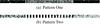 |
Fig. A.1 Last four pixels (from bottom to top). Shown are the two types of pattern that randomly show up on the SINFONI detector. When affected, it is always at least one amplifier (64 pixels or columns). |
Pattern two shows a sinusoidal noise pattern in every four columns of one amplifier (see second row of Figs. A.1 and A.2). The pattern was fitted best with a sine function that added an offset of half a π to the next column. This pattern occurs only in amplifiers 14, 16, 18, and 20, counting from left to right and starting with 1.
Both patterns were observed in separate, but also in the same exposure (data file), no superposition was observed. In one data file, an amplifier stopped showing a noise pattern after about 1000 rows.
We investigated the last three pixels in every column of the detector. These pixels are control pixels that are not exposed to light but suffer from the same electronic noise as the rest of the detector2. From these pixels, we were able to determine if there is a noise problem in the amplifier columns by standard and mean deviation methods. We separated the two problems, first correcting for the constant offset pattern, which is easier to determine. The complication here was the automated correction due to positive or negative ADU means combined with negative or positive constant offsets. After that we corrected for the sinusoidal pattern by fitting a two-dimensional sine with 16 columns and four rows making up the 64 channels of every amplifier. The noise was detected and corrected in 66 data files (science and calibration data). The correction was successful as shown in Fig. A.2. Weak noise patterns, which were not selected by our routines, can still make the resulting data files noisier, however, the difference to other noise sources (e.g., photon noise, readout noise) is almost not measurable.
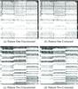 |
Fig. A.2 Parts of the detector where the pattern was detected a) and c) and then corrected b) and d). Note that the dark horizontal lines are part of an already known detector problem. The bright extended horizontal lines are OH sky lines. The three darkish extended vertical lines in a) and b) are the slit borders of the 32 slitlets on the detector. |
After correcting the unusual detector noise features we were confronted with a more typical problem, the OH emission of the atmosphere. Although we had exceptional weather conditions, photometric night, our 150 s exposures were too long for the fast changing atmospheric OH line emission. We used the SINFONI pipeline version 2.3.2 for data reduction, except for the OH correction. The usual OH correction performed by the pipeline resulted in strong OH residuals. By activating the higher density OH correction that was implemented following Davies (2007), the correction was better in some parts and worse in others, e.g., “P-Cygni” profiles in the OH lines were introduced. Comparing the raw target files with their pre/subsequent raw sky files, we registered a change in the strength of the OH lines from target to sky by up to 10%. In addition, a random shift of about 0.04 pixel in the spectral direction of the detector was noticed. We found this by fitting Gaussian profiles to several OH lines. We selected OH lines that had more than 100 peak counts above the continuum and that were isolated enough to assume a reliable profile fit. Furthermore, we selected OH lines from every vibrational transition. All selected lines in one detector column were fitted simultaneously to improve the continuum fit.
We found that all fitted lines in a sky file differed by about the same factor and pixel difference with respect to the corresponding target file, in every detector column. Hence, we took the median of all OH lines (41 in H- and 16 in K-band) and all 32 slits (about 60 of 64 pixels per slit were used) to determine the scaling factor and the shift of the OH lines. The fit did not work well at the edges of the slits due to contamination from the neighboring slit, hence we neglected the slit edges. As not to scale the continuum with the OH lines, we fitted the continuum in every detector column (spectral direction) and subtracted it before the OH line scaling. In H-band this was done by using a linear function. For
the K-band continuum we fitted a blackbody function, because the gray-body emission of the background becomes prominent at the red end of the K-band. We took the median of the fitted parameters over one slit to determine a robust continuum for the whole slit. After the subtraction of the continuum we scaled the remaining atmospheric emission features added back the continuum and then shifted the full column by the determined subpixel shift. The scaling was done based only on the emission lines because the continuum does not vary whereas the spectral shift has to be done on the full spectrum since the reason for the shift is a shear in the grating rather than some atmospheric effect.
We did not investigate in which amplifiers the pattern occurred exactly because the offset was sometimes very small. One could make it out by eye but the standard deviation was not much higher, if at all, than in unaffected amplifier columns. A lot more time would have been needed to investigate the exact occurrence of this noise pattern.
The first and last four pixels in every row and column are control pixels. We used only the last three in every column because in some exposures the first of the last four control pixels in a column seems to be slightly exposed, best seen in the fiber exposure data. In addition, we did not use the first four pixels in every column because the noise offset here was usually different and we could not combine the first and last pixels in every column, also the very first and fourth pixel sometimes suffered from other effects (e.g., slight exposure). The first and last pixels in every row are not interesting since this is a column-wise problem.
Acknowledgments
The authors kindly thank the staff at the Paranal Observatory for their assistance during the observation and the anonymous referee for fruitful comments and suggestions. This paper makes use of the following ALMA data: ADS/JAO.ALMA#2011.0.00208.S. ALMA is a partnership of ESO (representing its member states), NSF (USA) and NINS (Japan), together with NRC (Canada) and NSC and ASIAA (Taiwan), in cooperation with the Republic of Chile. The Joint ALMA Observatory is operated by ESO, AUI/NRAO and NAOJ. The National Radio Astronomy Observatory is a facility of the National Science Foundation operated under cooperative agreement by Associated Universities, Inc. We use data products from the Two Micron All Sky Survey, which is a joint project of the University of Massachusetts and the Infrared Processing and Analysis Center/California Institute of Technology, funded by the National Aeronautics and Space Administration and the National Science Foundation. We used observations made with the NASA/ESA Hubble Space Telescope, obtained from the data archive at the Space Telescope Institute. STScI is operated by the association of Universities for Research in Astronomy, Inc. under NASA contract NAS 5-26555. We used observations made with the NASA/ESA Hubble Space Telescope, and obtained from the Hubble Legacy Archive, which is a collaboration between the Space Telescope Science Institute (STScI/NASA), the Space Telescope European Coordinating Facility (ST-ECF/ESA), and the Canadian Astronomy Data Centre (CADC/NRC/CSA). This work was supported in part by the Deutsche Forschungsgemeinschaft (DFG) via the Cologne Bonn Graduate School (BCGS), and via grant SFB 956, as well as by the Max Planck Society and the University of Cologne through the International Max Planck Research School (IMPRS) for Astronomy and Astrophysics and by the German federal department for education and research (BMBF) under project number 50OS1101. We had fruitful discussions with members of the European-Union-funded COST Action MP0905: Black Holes in a violent Universe, and the COST Action MP1104: Polarization as a tool to study the Solar System and beyond. We received funding from the European Union Seventh Framework Programme (FP7/2007-2013) under grant agreement No.312789.
References
- Alonso-Herrero, A., Rieke, M. J., Rieke, G. H., & Ruiz, M. 1997, ApJ, 482, 747 [NASA ADS] [CrossRef] [Google Scholar]
- Alonso-Herrero, A., Rieke, G. H., Rieke, M. J., & Kelly, D. M. 2003, AJ, 125, 1210 [NASA ADS] [CrossRef] [Google Scholar]
- Bajaja, E., Wielebinski, R., Reuter, H.-P., Harnett, J. I., & Hummel, E. 1995, A&AS, 114, 147 [NASA ADS] [Google Scholar]
- Barteldrees, A., & Dettmar, R.-J. 1994, A&AS, 103, 475 [NASA ADS] [Google Scholar]
- Bedregal, A. G., Colina, L., Alonso-Herrero, A., & Arribas, S. 2009, ApJ, 698, 1852 [NASA ADS] [CrossRef] [Google Scholar]
- Bell, E. F., & de Jong, R. S. 2001, ApJ, 550, 212 [NASA ADS] [CrossRef] [Google Scholar]
- Bizyaev, D., & Mitronova, S. 2002, A&A, 389, 795 [NASA ADS] [CrossRef] [EDP Sciences] [Google Scholar]
- Bizyaev, D., & Mitronova, S. 2009, ApJ, 702, 1567 [NASA ADS] [CrossRef] [Google Scholar]
- Black, J. H., & van Dishoeck, E. F. 1987, ApJ, 322, 412 [NASA ADS] [CrossRef] [Google Scholar]
- Bonnet, H., Abuter, R., Baker, A., et al. 2004, The Messenger, 117, 17 [NASA ADS] [Google Scholar]
- Boone, F., Baker, A. J., Schinnerer, E., et al. 2007, A&A, 471, 113 [NASA ADS] [CrossRef] [EDP Sciences] [Google Scholar]
- Brand, P. W. J. L., Toner, M. P., Geballe, T. R., et al. 1989, MNRAS, 236, 929 [NASA ADS] [CrossRef] [Google Scholar]
- Buta, R. 1986, ApJS, 61, 631 [NASA ADS] [CrossRef] [Google Scholar]
- Buta, R., Ryder, S. D., Madsen, G. J., et al. 2001, AJ, 121, 225 [NASA ADS] [CrossRef] [Google Scholar]
- Buta, R. J., Sheth, K., Regan, M., et al. 2010, ApJS, 190, 147 [NASA ADS] [CrossRef] [Google Scholar]
- Calzetti, D. 1997, AJ, 113, 162 [NASA ADS] [CrossRef] [Google Scholar]
- Casasola, V., Combes, F., García-Burillo, S., et al. 2008, A&A, 490, 61 [NASA ADS] [CrossRef] [EDP Sciences] [Google Scholar]
- Casasola, V., Hunt, L. K., Combes, F., et al. 2010, A&A, 510, 52 [Google Scholar]
- Cid Fernandes, R., Storchi-Bergmann, T., & Schmitt, H. R. 1998, MNRAS, 297, 579 [NASA ADS] [CrossRef] [Google Scholar]
- Cid Fernandes, R., Gu, Q., Melnick, J., et al. 2004, MNRAS, 355, 273 [NASA ADS] [CrossRef] [Google Scholar]
- Combes, F., García-Burillo, S., Boone, F., et al. 2004, A&A, 414, 857 [NASA ADS] [CrossRef] [EDP Sciences] [Google Scholar]
- Combes, F., Baker, A. J., Schinnerer, E., et al. 2009, A&A, 503, 73 [NASA ADS] [CrossRef] [EDP Sciences] [Google Scholar]
- Combes, F., García-Burillo, S., Casasola, V., et al. 2013, A&A, 558, A124 [NASA ADS] [CrossRef] [EDP Sciences] [Google Scholar]
- Combes, F., García-Burillo, S., Casasola, V., et al. 2014, A&A, 565, A97 [NASA ADS] [CrossRef] [EDP Sciences] [Google Scholar]
- Davies, R. I. 2007, MNRAS, 375, 1099 [NASA ADS] [CrossRef] [Google Scholar]
- Davies, R. I., Thomas, J., Genzel, R., et al. 2006, ApJ, 646, 754 [NASA ADS] [CrossRef] [Google Scholar]
- Davies, R. I., Müller Sánchez, F., Genzel, R., et al. 2007, ApJ, 671, 1388 [NASA ADS] [CrossRef] [Google Scholar]
- Draine, B. T., & McKee, C. F. 1993, Ann. Rev. Astron. Astrophys., 31, 373 [Google Scholar]
- Draine, B. T., & Woods, D. T. 1990, ApJ, 363, 464 [NASA ADS] [CrossRef] [Google Scholar]
- Eckart, A., Schinnerer, E., & Tacconi, L. 2000, New Astron. Rev., 44, 523 [Google Scholar]
- Eckart, A., Schinnerer, E., & Staguhn, J. 2001, in Proc. IAU Symp., 205, 344 [Google Scholar]
- Eisenhauer, F., Abuter, R., Bickert, K., et al. 2003, in Proc. SPIE 4841, eds. M. Iye, & A. F. M. Moorwood, 1548 [Google Scholar]
- Emsellem, E., Greusard, D., Combes, F., et al. 2001, A&A, 368, 52 [NASA ADS] [CrossRef] [EDP Sciences] [Google Scholar]
- Esquej, P., Alonso-Herrero, A., González-Martín, O., et al. 2014, ApJ, 780, 86 [Google Scholar]
- Falcón-Barroso, J., Bacon, R., Bureau, M., et al. 2006, MNRAS, 369, 529 [NASA ADS] [CrossRef] [Google Scholar]
- Ferrarese, L., & Merritt, D. 2000, ApJ, 539, L9 [NASA ADS] [CrossRef] [Google Scholar]
- Fisher, D. B., & Drory, N. 2010, ApJ, 716, 942 [NASA ADS] [CrossRef] [Google Scholar]
- García-Burillo, S., Combes, F., Hunt, L. K., et al. 2003, A&A, 407, 485 [NASA ADS] [CrossRef] [EDP Sciences] [Google Scholar]
- García-Burillo, S., Combes, F., Schinnerer, E., Boone, F., & Hunt, L. K. 2005, A&A, 441, 1011 [NASA ADS] [CrossRef] [EDP Sciences] [Google Scholar]
- García-Burillo, S., Fernández-García, S., Combes, F., et al. 2009, A&A, 496, 85 [NASA ADS] [CrossRef] [EDP Sciences] [Google Scholar]
- Gültekin, K., Richstone, D. O., Gebhardt, K., et al. 2009, ApJ, 698, 198 [NASA ADS] [CrossRef] [Google Scholar]
- Howell, S. B. 2000, Handbook of CCD Astronomy (New York: Cambridge University Press) [Google Scholar]
- Hunt, L. K., Combes, F., García-Burillo, S., et al. 2008, A&A, 482, 133 [NASA ADS] [CrossRef] [EDP Sciences] [Google Scholar]
- Irwin, J. A., Wilson, C. D., Wiegert, T., et al. 2011, MNRAS, 410, 1423 [NASA ADS] [Google Scholar]
- Israel, F. P., Tilanus, R. P. J., & Baas, F. 2006, A&A, 445, 907 [NASA ADS] [CrossRef] [EDP Sciences] [Google Scholar]
- Jungwiert, B., Combes, F., & Axon, D. J. 1997, A&AS, 125, 479 [NASA ADS] [CrossRef] [EDP Sciences] [Google Scholar]
- Kilborn, V. A., Koribalski, B. S., Forbes, D. A., Barnes, D. G., & Musgrave, R. C. 2005, MNRAS, 356, 77 [NASA ADS] [CrossRef] [Google Scholar]
- Koribalski, B. S., Staveley-Smith, L., Kilborn, V. A., et al. 2004, AJ, 128, 16 [NASA ADS] [CrossRef] [Google Scholar]
- Krips, M., Eckart, A., Neri, R., et al. 2005, A&A, 442, 479 [NASA ADS] [CrossRef] [EDP Sciences] [Google Scholar]
- Lindt-Krieg, E., Eckart, A., Neri, R., et al. 2008, A&A, 479, 377 [NASA ADS] [CrossRef] [EDP Sciences] [Google Scholar]
- Liu, J.-F., & Bregman, J. N. 2005, ApJS, 157, 59 [NASA ADS] [CrossRef] [Google Scholar]
- Magorrian, J., Tremaine, S., Richstone, D., et al. 1998, AJ, 115, 2285 [NASA ADS] [CrossRef] [Google Scholar]
- Maiolino, R., Rieke, G. H., & Rieke, M. J. 1996, AJ, 111, 537 [NASA ADS] [CrossRef] [Google Scholar]
- Maloney, P. R., Hollenbach, D. J., & Tielens, A. G. G. M. 1996, ApJ, 466, 561 [NASA ADS] [CrossRef] [Google Scholar]
- Maoz, D., Filippenko, A. V., Ho, L. C., et al. 1996, ApJS, 107, 215 [NASA ADS] [CrossRef] [Google Scholar]
- Mauersberger, R., Henkel, C., Walsh, W., & Schulz, A. 1999, A&A, 341, 256 [NASA ADS] [Google Scholar]
- Mazzalay, X., Saglia, R. P., Erwin, P., et al. 2013, MNRAS, 428, 2389 [NASA ADS] [CrossRef] [Google Scholar]
- McMullin, J. P., Waters, B., Schiebel, D., Young, W., & Golap, K. 2007, in ASP Conf. Ser., 376, 127 [Google Scholar]
- Muraoka, K., Kohno, K., Tosaki, T., et al. 2007, PASJ, 59, 43 [NASA ADS] [Google Scholar]
- Nussbaumer, H., & Storey, P. J. 1988, A&A, 193, 327 [NASA ADS] [Google Scholar]
- Panuzzo, P., Bressan, A., Granato, G. L., Silva, L., & Danese, L. 2003, A&A, 409, 99 [NASA ADS] [CrossRef] [EDP Sciences] [Google Scholar]
- Peeples, M. S., & Martini, P. 2006, ApJ, 652, 1097 [NASA ADS] [CrossRef] [Google Scholar]
- Rodríguez-Ardila, A., Pastoriza, M. G., Viegas, S., Sigut, T. A. A., & Pradhan, A. K. 2004, A&A, 425, 457 [NASA ADS] [CrossRef] [EDP Sciences] [Google Scholar]
- Rodríguez-Ardila, A., Riffel, R., & Pastoriza, M. G. 2005, MNRAS, 364, 1041 [NASA ADS] [CrossRef] [Google Scholar]
- Rosenberg, M. J. F., van der Werf, P. P., & Israel, F. P. 2012, A&A, 540, A116 [NASA ADS] [CrossRef] [EDP Sciences] [Google Scholar]
- Ryder, S. D., Buta, R. J., Toledo, H., et al. 1996, ApJ, 460, 665 [NASA ADS] [CrossRef] [Google Scholar]
- Sànchez-Bàzquez, P., Ocvirk, P., Gibson, B. K., Pérez, I., & Peletier, R. F. 2011, MNRAS, 415, 709 [NASA ADS] [CrossRef] [Google Scholar]
- Schödel, R., Ott, T., Genzel, R., et al. 2002, Nature, 419, 694 [NASA ADS] [CrossRef] [PubMed] [Google Scholar]
- Schödel, R., Merritt, D., & Eckart, A. 2009, A&A, 502, 91 [NASA ADS] [CrossRef] [EDP Sciences] [Google Scholar]
- Scoville, N. Z., Hall, D. N. B., Ridgway, S. T., & Kleinmann, S. G. 1982, ApJ, 253, 136 [NASA ADS] [CrossRef] [Google Scholar]
- Sheth, K., Vogel, S. N., Regan, M. W., Thornley, M. D., & Teuben, P. J. 2005, ApJ, 632, 217 [NASA ADS] [CrossRef] [Google Scholar]
- Smajić, S., Fischer, S., Zuther, J., & Eckart, A. 2012, A&A, 544, A105 [NASA ADS] [CrossRef] [EDP Sciences] [Google Scholar]
- Solomon, P. M., & Barrett, J. W. 1991, in Proc. IAU Symp. (Dordrecht: Kluwer Academic Publishers), 146, 235 [Google Scholar]
- Sosa-Brito, R. M., Tacconi-Garman, L. E., Lehnert, M. D., & Gallimore, J. F. 2001, ApJS, 136, 61 [NASA ADS] [CrossRef] [Google Scholar]
- Staguhn, J., Schinnerer, E., & Eckart, A. 2001, in Proc. IAU Symp., 205, 340 [Google Scholar]
- Sternberg, A., & Dalgarno, A. 1989, ApJ, 338, 197 [NASA ADS] [CrossRef] [Google Scholar]
- Tilanus, R. P. J., Tacconi, L. J., Sutton, E. C., et al. 1991, ApJ, 376, 500 [NASA ADS] [CrossRef] [Google Scholar]
- Tine, S., Lepp, S., Gredel, R., & Dalgarno, A. 1997, ApJ, 481, 282 [NASA ADS] [CrossRef] [Google Scholar]
- Turner, E. L., & Ostriker, J. P. 1977, ApJ, 217, 24 [NASA ADS] [CrossRef] [Google Scholar]
- Valencia-S., M., Zuther, J., Eckart, A., et al. 2012, A&A, 544, A129 [NASA ADS] [CrossRef] [EDP Sciences] [Google Scholar]
- van der Laan, T. P. R., Schinnerer, E., Boone, F., et al. 2011, A&A, 529, A45 [NASA ADS] [CrossRef] [EDP Sciences] [Google Scholar]
- Véron-Cetty, M.-P., & Véron, P. 1986, A&AS, 65, 241 [NASA ADS] [Google Scholar]
- Wada, K., & Tomisaka, K. 2005, ApJ, 619, 93 [NASA ADS] [CrossRef] [Google Scholar]
- Wilson, C. D., Warren, B. E., Israel, F. P., et al. 2009, ApJ, 693, 1736 [NASA ADS] [CrossRef] [Google Scholar]
- Winge, C., Riffel, R. A., & Storchi-Bergmann, T. 2009, ApJS, 185, 186 [NASA ADS] [CrossRef] [Google Scholar]
- Wolniewicz, L., Simbotin, I., & Dalgarno, A. 1998, ApJS, 115, 293 [NASA ADS] [CrossRef] [Google Scholar]
- Wozniak, H., Friedli, D., Martinet, L., Martin, P., & Bratschi, P. 1995, A&AS, 111, 115 [NASA ADS] [Google Scholar]
- Zuther, J., Iserlohe, C., Pott, J.-U., et al. 2007, A&A, 466, 451 [NASA ADS] [CrossRef] [EDP Sciences] [Google Scholar]
All Tables
All Figures
|
Fig. 1 HST F438 wide field image of NGC 1433 from the ESA Hubble Science Archive. The FOV of 10″× 10″ of our SINFONI observations is marked by a square. The color scale in the lower image was chosen to reflect the large scale structure of the host, e.g., the main stellar bar. The top image shows the prominent dust lanes in the center of NGC 1433. |
| In the text | |
|
Fig. 2 Shown are Gaussian fits to radial luminosity profiles of the K-band standard star continuum, the H-band standard star continuum, the H- and K-bands galaxy continuum, the fitted stellar continuum in the K-band, Fe ii λ1.644 μm, and Brγ. Note that K-band galaxy continuum and the fitted stellar continuum lie on top of each other. The Gaussian fit was centered on the galactic center. |
| In the text | |
|
Fig. 3 Flux [10-20 W m-2], FWHM [km s-1], and LOSV [km s-1] maps (left to right) of the [Fe ii], Brγ, and H2λ(1−0)S(1) lines (top to bottom). a) and g) show the beam size in the lower left corner for H- and K-band respectively. g) Shows the aperture sizes taken for our measurements. One angular resolution element (beam) corresponds to a PSFFWHM of 0 |
| In the text | |
|
Fig. 4 ALMA cycle 0 molecular 12CO(3−2) maps. a) Emission map of 12CO(3−2) [Jy beam-1 km s-1] overlaid with H2(1−0)S(1) emission contours. The red ellipse at −4,4 describes the beam size. The dispersion (moment 2) is shown in b) and the LOSV is shown in c), both maps are in [km s-1]. c) Cuts for the position velocity (PV) diagrams (see Fig. 12). The cuts were not set on the galactic center but along the central velocity gradient of the 12CO(3−2) 1st moment map. |
| In the text | |
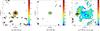 |
Fig. 5 EW maps of the narrow Brγ, [Fe ii], and H2λ(1−0)S(1) lines in Å. For details, see Sect. 3. |
| In the text | |
|
Fig. 6 H − K color diagram in magnitudes showing the center of NGC 1433 measured in the SINFONI H- and K-band. The contours are from the 0.87 mm continuum emission measured by ALMA. For detail, see Sects. 3.3 and 4.1. |
| In the text | |
|
Fig. 7 The fit over the stellar dispersion from the continuum decomposition in 5 kms-1 bins. The X-axis shows the fitted dispersion and the Y-axis the total number of spatial pixels that corresponds to this dispersion bin. The red curve represents a Gaussian fit to the distribution. |
| In the text | |
|
Fig. 8 From left to right H-band, K-band [10-18 W m-2μm-1], and 0.87 mm [Jy beam-1] continuum. c) H2(1−0)S(1) contour overlaid on the 3 sigma clipped 0.87 mm continuum. For details, see Sects. 3.3 and 4.1. |
| In the text | |
|
Fig. 9 a) Fitted stellar LOSV map [km s-1], b) stellar disperion [km s-1], and c) stellar continuum (arbitrary unit) map. In panel a) the LOSV PA of the galactic rotation is marked. Panel c) shows probable PAs of the isophotes where the largest cross marks the PA of the nuclear bar and the smallest cross the orientation of the beam. The middle cross indicates a possible twist in the isophotal lines. |
| In the text | |
|
Fig. 10 a) An HST map at about 4380 Å with H2(1−0)S(1) contours overlaid. b) Same HST image in the ALMA FOV with the 12CO(3−2) line emission in contours. The HST images were taken from the archive and were observed with the WFC3 instrument and the UVIS detector using the F438W filter. The images illustrate the remarkable overlap of dust lanes and molecular hydrogen a) and 12CO(3−2) emission b), respectively. |
| In the text | |
|
Fig. 11 Stellar LOSV subtracted maps of H2(1−0)S(1) and 12CO(3−2). c) is the same as b) but 20 km s-1 were added to the residual to indicate the higher resemblance with panel a). All color-bar units are in km s-1. For details, see Sect. 4.2. |
| In the text | |
|
Fig. 12 PV diagrams from the 12CO(3−2) ALMA cube a) along the central velocity gradient (PA = 140°) and b) perpendicular to the central velocity gradient (PA = 50°). The color-bar shows the flux density in [Jy beam-1]. The position of the cuts is displayed in Fig. 4c. The white rectangle marks the nuclear region in which the central velocity gradient is dominant. (a1) to (b3) mark dust arm positions: (a1) eastern arm, (a2) southern arm, (a3) nuclear arm, (a4) northern arm, (b1) overlap between eastern and southern arm, (b2) nuclear arm, (b3) southern arm (west). |
| In the text | |
|
Fig. 13 Models used in Sect. 4.2.1 are presented: a)−b) are the constructed models, d)−f) are the PSF convolved models. For details, see Sect. 4.2.1. |
| In the text | |
|
Fig. 14 a) Shows the central 4″ × 4″. b) Shows the same detail but subtracted by the combined model (see Fig. 13f). For details, see Sect. 4.2.1. |
| In the text | |
|
Fig. 15 Top: strengths (Qm and total QT) of the m = 1 to m = 4 Fourier components of the stellar potential within the central kpc. Inside a radius of 130 pc, the m = 1 term dominates, and the nuclear bar extends until 350 pc radius. Bottom: corresponding phases in radians of the Fourier components, taken from the major axis, in the deprojected image. |
| In the text | |
|
Fig. 16 Top: map of the gravitational torque, t(x,y) × Σ(x,y), weighted by the gas surface density Σ, assumed proportional to the 12CO(3−2) emission. The torque per unit mass is t(x,y) = xFy − yFx at each pixel (x, y), where Fx and Fy are the forces per unit mass, derived from the potential. The torques change sign as expected in a four-quadrant pattern (or butterfly diagram). The orientation of the quadrants follows the nuclear bar’s orientation. In this deprojected picture, the major axis of the galaxy is oriented parallel to the horizontal axis. The inclined line reproduces the mean orientation of the bar (PA = 101° on the deprojected image). Bottom: deprojected image of the 12CO(3−2) emission, at the same scale, and with the same orientation, for comparison. The axes are labeled in arcseconds relative to the center. The color scales are linear, in arbitrary units. |
| In the text | |
|
Fig. 17 Radial distribution of the torque, quantified by the fraction of the angular momentum transferred from the gas in one rotation, dL/L, estimated from the 12CO(3−2) deprojected map. The vertical line at 88 pc radius delimits the extent of the central gas outflow, and the computation has no meaning here. The torque is positive inside a 200 pc radius and then negative outside. |
| In the text | |
|
Fig. 18 Diagnostic diagram to classify the emission at the nucleus. The [Fe ii] λ1.257 μm and Paβ values were derived from the [Fe ii] λ1.644 μm and the Brγ line. |
| In the text | |
|
Fig. 19 Molecular hydrogen diagnostic diagram to classify the emission at the nucleus in red and in emission spots sp(A) in green and sp(B) in blue. Line ratios are H2(2−1)S(1)/H2(1−0)S(1) and H2(1−0)S(3)/H2(1−0)S(1). The curve represents thermal emission at 1000–3000 K. Horizontal stripes are thermal UV excitation models by Sternberg & Dalgarno (1989). Vertical stripes are non-thermal models by Black & van Dishoeck (1987). The area of X-ray heating models by Draine & Woods (1990) is marked by an open triangle (yellow). The open turquoise circle marks the region of the shock model by Brand et al. (1989). |
| In the text | |
|
Fig. A.1 Last four pixels (from bottom to top). Shown are the two types of pattern that randomly show up on the SINFONI detector. When affected, it is always at least one amplifier (64 pixels or columns). |
| In the text | |
|
Fig. A.2 Parts of the detector where the pattern was detected a) and c) and then corrected b) and d). Note that the dark horizontal lines are part of an already known detector problem. The bright extended horizontal lines are OH sky lines. The three darkish extended vertical lines in a) and b) are the slit borders of the 32 slitlets on the detector. |
| In the text | |
Current usage metrics show cumulative count of Article Views (full-text article views including HTML views, PDF and ePub downloads, according to the available data) and Abstracts Views on Vision4Press platform.
Data correspond to usage on the plateform after 2015. The current usage metrics is available 48-96 hours after online publication and is updated daily on week days.
Initial download of the metrics may take a while.