| Issue |
A&A
Volume 567, July 2014
|
|
|---|---|---|
| Article Number | A48 | |
| Number of page(s) | 14 | |
| Section | Planets and planetary systems | |
| DOI | https://doi.org/10.1051/0004-6361/201323102 | |
| Published online | 09 July 2014 | |
A vigorous activity cycle mimicking a planetary system in HD 200466⋆,⋆⋆
1
INAF – Osservatorio Astronomico di Padova, Vicolo dell’Osservatorio
5,
35122
Padova,
Italy
e-mail:
This email address is being protected from spambots. You need JavaScript enabled to view it.
2
Dipartimento di Astronomia – Universitá di Padova,
Vicolo dell’Osservatorio 2,
Padova,
Italy
3
Fundación Galileo Galilei – INAF, Rambla José Ana Fernandez Pérez
7, 38712
Breña Baja,
Spain
4
Dipartimento di Fisica – Universitá di Padova,
via Marzolo 8, Padova, Italy
5
McDonald Observatory, The University of Texas at
Austin, Austin
TX
78712,
USA
6
INAF – Osservatorio Astrofisico di Catania, via S. Sofia
78, Catania,
Italy
Received: 21 November 2013
Accepted: 20 May 2014
Abstract
Stellar activity can be a source of radial velocity (RV) noise and can reproduce periodic RV variations similar to those produced by an exoplanet. We present the vigorous activity cycle in the primary of the visual binary HD 200466, a system made of two almost identical solar-type stars with an apparent separation of 4.6 arcsec at a distance of 44 ± 2 pc. High precision RV over more than a decade, adaptive optics (AO) images, and abundances have been obtained for both components. A linear trend in the RV is found for the secondary. We assumed that it is due to the binary orbit and once coupled with the astrometric data, it strongly constrains the orbital solution of the binary at high eccentricities (e ~ 0.85) and quite small periastron of ~21 AU. If this orbital motion is subtracted from the primary radial velocity curve, a highly significant (false alarm probability <0.1%) period of about 1300 d is obtained, suggesting in a first analysis the presence of a giant planet, but it turned out to be due to the stellar activity cycle. Since our spectra do not include the Ca II resonance lines, we measured a chromospheric activity indicator based on the Hα line to study the correlation between activity cycles and long-term activity variations. While the bisector analysis of the line profile does not show a clear indication of activity, the correlation between the Hα line indicator and the RV measurements identify the presence of a strong activity cycle.
Key words: stars: individual: HD 200466 / binaries: visual / stars: activity / stars: abundances / techniques: radial velocities / techniques: high angular resolution
Based on observations made with the Italian Telescopio Nazionale Galileo (TNG) operated on the island of La Palma by the Fundación Galileo Galilei of the Istituto Nazionale di Astrofisica (INAF) at the Spanish Observatorio del Roque de los Muchachos of the Instituto de Astrofísica de Canarias.
Tables 5 and 6 are available in electronic form at http://www.aanda.org
© ESO, 2014
1. Introduction
The impact of star spots on high precision radial velocity (RV) surveys on rotational timescales is well documented by several observational detections collected in the past years (see e.g. Queloz et al. 2001; and Paulson et al. 2004). Various authors explained such observations by means of theoretical modelling (Saar & Donahue 1997; Hatzes 2002; Desort et al. 2007). On the other hand, the impact of solar-like activity cycles on high-precision RVs has been studied only recently by analysing the correlations between observed jitter and chromospheric activity for the stars in the California Planet Search (Isaacson & Fischer 2010) or by computing chromospheric activity indicators based on some element lines as in the HARPS program (Gomes da Silva et al. 2011). Some authors proposed several methods and models to reduce the associated noise (Dumusque et al. 2011; Meunier & Lagrange 2013) and predict the activity-induced RV variations (Lanza et al. 2011).
Active regions are known to affect the convection pattern in the Sun, with effects on line bisectors and line shifts, possibly mimicking the low-amplitude RV variations due to extrasolar planets (Dravins 1992).
Meunier et al. (2010) and Meunier & Lagrange (2013) used the spots and plages observed on the Sun over a solar cycle to derive the expected RV signature. They considered both the photometric contribution of spots and plages and the contribution of the latter due to the attenuation of the convective blueshift, which is the dominant source of RV variability, with peak-to-valley amplitude of about 8–10 m/s over a solar cycle. Boisse et al. (2011) simulated dark spots on a rotating stellar photosphere in order to better understand and characterize the effects of stellar activity and to differentiate them from planetary signals. Their approach was also applied to and validated on four active planet-host stars. Useful results were obtained, providing some constraints on the planet period, on semi-amplitude of the planet, on star rotational period, and on data covering. Saar & Fischer (2000) looked for correlations between the strength of the Ca II infrared triplet and RV in the Lick planet search data and found significant correlations in about 30% of the stars. They also aimed at correcting the RVs for the effects of magnetic activity using these correlations. They found that less active stars with significant Ca II variations are those that are best corrected. These variations were explained as due to long-term activity cycles, while corrections become less reliable at increasing activity levels when short-term noise due to star-spots becomes the dominant source of RV variations. It should be noticed that plages affecting convection do not only produce a RV signal on long-term scales (cycle), but also produces a modulation due to rotation period, on smaller timescales.
In Isaacson & Fischer (2010) the ΔS index of excess emission in the core of Ca II H&K lines was defined and correlated to the RV jitter, as a function of the star B − V colour. They found that chromospherically quiet F and G dwarfs and subgiants exhibit higher baseline levels of the astrophysical jitter than K dwarfs. They also concluded that the correlation between the activity cycle and the Doppler measurements is rare to see, making the correction of activity-induced velocity variations in F and G dwarf difficult.
Recently, Lovis et al. (2011) studied the magnetic activity cycles in solar-type stars in the HARPS program analysing the Ca II H&K lines. They found that 39% of the old solar-type stars in the solar neighbourhood do not show any activity cycles, while 61% do have one. They also confirmed that the sensitivity of RVs to magnetic cycles increases towards hotter stars, while late K dwarfs are almost insensitive (confirming the result of Isaacson & Fischer 2010). For the HARPS sample they concluded that the activity cycles can induce RV variations having long period and amplitude up to about 25 m/s.
From the line analysis on a sample of M dwarf stars from the HARPS program, about 40% of the stellar sample showed significant variability. Gomes da Silva et al. (2011) concluded that Hα shows good correlation with SCa II for the most active stars, indicating that the correlation between Ca II and Hα depends on the activity level of the star. The correlation between different activity indicators is complex and can be different depending on the star (Cincunegui et al. 2007; see also Meunier & Delfosse 2009).
Therefore care should be taken in the claim of detection of planets around active stars. False alarms have been reported in the past (see e.g. Hernan-Obispo et al. 2010; Figueira et al. 2010; Setiawan et al. 2008; Huelamo et al. 2008) and controversial cases for which conclusive evidence of the Keplerian origin of the RV variations is still lacking have been discussed in e.g. Hatzes & Cochran (1998). The measurements of activity indicators and line profile variations on the same spectra used for the determination of high-precision RVs are crucial to disentangling RV variations due to Keplerian motions from those related to magnetic activity. Calcium II H&K lines represent the most widely used chromospheric activity indicator for solar-type stars. For these stars, Hα has been mostly neglected but it is a suitable alternative when Ca II H&K lines are not included in the spectra used for RV determination. Line profiles are also sensitive to phenomena related to magnetic activity. Furthermore, they are a unique diagnostic for checking the occurrence of contamination in binary systems (Martinez Fiorenzano et al. 2005; Torres et al. 2004).
Within our survey looking for giant planets in nearly equal mass visual binaries with the SARG spectrograph at Telescopio Nazionale Galileo (TNG; Desidera et al. 2010), we discovered an interesting system (HD 200466) where the primary exhibits large variations of the RVs that are correlated with variations of activity indicators, while the secondary only shows a long-term trend in RVs. While almost twin late-G dwarfs, the two stars also have other differences, markedly in the photospheric Li abundance. This paper presents the observations of this system. The paper is organized as follows. In Sect. 2 we describe the observations and reduction of the spectroscopic and adaptive optics data. We also present the analysis of the Hα line performed to detect the presence of stellar activity. In Sect. 3 we describe the stellar parameters of each component. In Sect. 4 we present the RV variations for both components. In Sect. 5 we present the clues of the binary orbital solution and the plausible system architecture. In Sect. 6 we assume and analyse the presence of a planet around the primary component. In Sect. 7 we argue that the RV variations observed in HD 200466A are related to the stellar activity cycle. In Sect. 8 we consider approaches to correct the RV time series for the effects of chromospheric activity. In Sect. 9 we discuss the results in the context of the possible effect of the presence of planets on the lithium content of solar-type stars and summarize our conclusions.
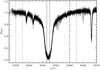 |
Fig. 1 Hα profile of a sample of 30 spectra of HD 200466A. The dotted lines correspond to the two ranges used to calculate the normalized continuum. The solid line corresponds to the “on line” band used for the activity analysis. |
2. Observations and data reduction
2.1. High resolution spectroscopy with SARG
Spectroscopic observations were performed using SARG, the high resolution spectrograph of TNG (Gratton et al. 2001). The instrument set up is described in Desidera et al. (2011). Integration time was fixed at 900 s to keep errors due to the lack of knowledge of flux mid-time of each exposure below photon noise. Typical signal-to-noise ratio (S/N) at about 5800 Å is about 100 per pixel. Overall, 76 and 72 spectra of HD 200466 A and B, respectively, were acquired from September 2000 to September 2011.
Data reduction was performed in a standard way using IRAF. However for the Hα analysis we used an “ad hoc” continuum normalization of spectra, because this broad line is located close to the blue edge of the order 93 of SARG echelle spectra. Since the spectral line is very broad, the standard IRAF procedure to fit a polynomial through the highest spectral point is not adequate. In order to extract information on this line flux we then calculated the continuum separately from the standard IRAF data reduction (see Fig. 1).
Radial velocities were obtained using the AUSTRAL code (Endl et al. 2000). Internal errors of RVs are typically about 4 m/s. Tables 5 and 6 list the RVs for HD 200466 A and B, respectively.
Average line profiles were also derived to get additional diagnostics of spurious RV variations due to stellar activity, contamination, or other causes. We followed the approach developed in Martinez Fiorenzano et al. (2005), but considering a more extended line list with respect to previous analysis to build the mask involved in the CCF calculation. The top and bottom zones for the calculations of the bisector velocity span (BVS) were set as follows: top centred at 25% of the maximum absorption, bottom at 87%; in both cases the width was of 25%. The BVS are listed in Cols. 4 and 5 of Tables 5 and 6, with their errors.
The analysis of the Hα line was performed to detect the presence of stellar activity. The approach used is based on measuring an ad hoc flux index in the line as well as in adjacent continuum bands on both the short and long wavelength wings for each spectra of both companions (see e.g. Fig. 1). The values for this index are also listed in Cols. 6 and 7 of Tables 5 and 6, with their errors.
2.2. Direct imaging with TNG/AdOpt
2.2.1. Observations
To complement the spectroscopic data, HD 200466 was observed on July 12 and 20, 2007, and Aug. 9, 2008, with TNG/AdOpt, the adaptive optics module of TNG (Cecconi et al. 2006). The instrument feeds the HgCdTe Hawaii 1024 × 1024 detector of NICS, the near infrared camera, and spectrograph of TNG, providing a field of view (FoV) of about 44 × 44 arcsec, with a pixel scale of 0.0437′′/pixel. Plate scale and absolute detector orientation were derived as part of the program of follow-up of systems shown to have long-term RV trends from the SARG planet search (see Desidera et al. 2010, for some preliminary results). We did not find significant variations of the plate scale with time, while the angular offset between the nominal detector orientation and the true direction of north was found to have small but significant differences between the 2007 and 2008 seasons, likely due to the refurbishment of the instrument made during the 2007–2008 winter. As our program with TNG/AdOpt is focused on the follow-up of stars that show long-term RV trends, in several cases we expect the occurrence of detectable astrometric variations induced by the companion. The final value of the plate scale depends very little on the choice of the subsample used to derive it (all targets or only the few systems without large RV trends), but the dispersion is instead much larger when all the targets are included. Furthermore, we are working on the determination and correction of the optical distortions. At the three observing epochs we acquired 118, 134, and 98 images on HD 200466 in Brγ intermediate-band filtre, avoiding detector saturation. At each epoch, observations with different instrument rotation images were obtained. This makes the optimization of the position shift between the images of the components easier and provides meaningful results as close as possible to the stars. The primary was used as the reference star for the adaptive optics. The target was observed in different positions on the detector for sky subtraction purposes, and at two or three orientations of the FoV on each run to allow a better disentangling between true companions and instrumental artefacts.
2.2.2. Data analysis procedure
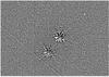 |
Fig. 2 Residuals on the composite TNG/AdOpt image after subtraction of the two components of the HD 200466 system. |
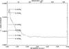 |
Fig. 3 Detection limits from TNG/AdOpt images of HD 200466. The contrast in the Brγ band is shown as a function of projected separation in arcsec and AU. Corresponding values of mass limits are shown. |
The data analysis procedure is described in detail in Desidera et al. (2011) and we briefly summarize it here. We first corrected for detector cross-talk using the dedicated code developed at TNG1. Then we performed standard image preprocessing (flat fielding, bad pixels, and sky corrections) in the IRAF environment. In the data analysis, we exploit the similarity between the point spread functions (PSFs) of the two components and the availability of observations taken at different rotation angles. Datacubes of images taken with the same rotation angles were built and a median combined image was obtained, discarding images with large full width at half maximum. The resulting images for the three orientations were then rotated and summed together. To enhance detectability of faint companions at small projected separation, we considered the square regions in the final image composed of 51 × 51 pixels around the position of the two components, and subtracted each of them to the other after scaling them for the flux difference. This PSF subtraction procedure works quite well because the two stellar images are well within the isoplanatic angle. It allows a gain of about an order of magnitude in contrast at separation <1 arcsec. Figure 2 shows the image after the subtraction of the two components of the HD 200466 system. We did not find any evidence of faint companions to either of the two components. In Fig. 3 we display the limiting contrast obtained around the B component and the corresponding mass detection limits (see next paragraph). The limiting contrast was obtained considering 5 times the standard deviation in circular annuli around the calculated position of the star. During these calculations the A component was masked. We verified that the contrast curve agreed closely with a noise model which included speckle, photon, sky background, and detector noise. These detection limits were further validated by injecting a number of fake objects at different separations and at different contrast and performing the same analysis as on the original images.
To obtain the mass detection limits from the contrast limits we first transformed the luminosity contrast in absolute magnitude in the K band. For MK magnitudes brighter than 9.5 we used the mass–luminosity relation given in Delfosse et al. (2000) for low mass stars (M< 0.6 M⊙), obtaining a mass value for each magnitude limit. For MK in the range of 9.5 <MK< 12.8 we interpolated the tables by Chabrier et al. (2000) for the star age derived in Sect. 3 (2 Gyr) while for magnitudes fainter than MK 12.8 we used the same method but using the tables from Baraffe et al. (2003)2. To smooth the irregularities of three range of masses we fitted the distribution by using an exponential function reproducing the mass detection limits for each separation.
3. Stellar parameters
For a proper interpretation of the observed RV variability, a careful evaluation of the stellar properties is mandatory. Table 1 summarizes the stellar parameters of the components of HD 200466, that are described in more detail below.
3.1. Spectroscopic and photometric parameters
The abundance analysis performed in Desidera et al. (2004) relies on the absolute magnitudes for the derivation of stellar gravity (and then indirectly on the determination of effective temperatures using the ionization equilibrium). In that paper, we used the Hipparcos parallax (ESA 1997). We adopted the revised parallax distance published by Van Leuween (2007) and used the web interface of Padova stellar models param3 (Da Silva et al. 2006) to derive stellar masses in a fully self-consistent way. Then we repeated the abundance analysis. This produced results similar to the previous one (slightly cooler effective temperatures, and very similar temperature and abundance differences). The final atmospheric parameters and the adopted stellar masses are listed in Table 1.
As this analysis uses the trigonometric parallax and the stellar models, it cannot be considered an independent check of the reliability of the parallax and of the absolute effective temperature. To this purpose, we consider photometric colours and alternative spectroscopic determinations of effective temperatures.
Few high quality measurements of magnitudes of the two components are available in the literature. Combining them, Desidera et al. (2004) derived VA = 8.399 ± 0.005, VB = 8.528 ± 0.006, B − VA = 0.71 ± 0.02, and B − VB = 0.79 ± 0.03 mag. The colour difference of Tycho photometry for the two components is much larger than that expected from the magnitude (ΔV = 0.13) and spectroscopic temperature differences (ΔTeff = 53 K). Similar discrepancies are common for the pairs of our sample (see Desidera et al.2004, their Table 5). It is then likely that internal errors in Tycho colours for individual components have been underestimated for close binaries.
The V − K colours resulting from 2MASS photometry (Skrutskie et al. 2006) are probably not very accurate. They put both the components to the red of the main sequence for the appropriate metallicity by about 0.2 mag; furthermore, the secondary is marginally brighter in K. This is likely due to the uncertainties in 2MASS photometry which are much larger than the nominal ones for bright close binaries (aperture photometry on an unresolved object). Our AdOpt images yield a magnitude difference in the Brγ filtre of 0.10 mag (with the primary being brighter), as expected from the V mag difference4. As the resolved colours have significant errors, we consider composite photometry, that is available with high accuracy in the Hipparcos catalogue ((B − V)A + B = 0.748 ± 0.012, (V − I)A + B = 0.79 ± 0.01). From the composite colour and the observed V mag difference, assuming the stars follow a standard isochrone, we derived (B − V)A = 0.736, (B − V)B = 0.761, (V − I)A = 0.778, and (V − I)B = 0.801. These V − I and B − V colours are only slightly redder than the isochrone and would require shifts of just 0.05 and 0.10 mag in MV for (B − V) and (V − I) colours, respectively.
A fully spectroscopic analysis, deriving Teff from excitation equilibrium, yields temperatures that are cooler by about 120 K than those from ionization equilibrium (assuming nominal parallax) (5486 vs. 5603 K for HD 200466A), corresponding to a 0.20 mag shift in MV. All of this suggests that the trigonometric parallax is basically correct, although the system might be slightly closer than 44.4 pc. A distance closer than 40 pc is unlikely.
3.2. Lithium
Visual analysis of the spectra of HD 200466 A and B shows a significant difference in the 6708 Å Li doublet. We performed spectral synthesis of this spectral region to determine the Lithium abundance. We adopted the atmospheric parameters resulting from the updated abundance analysis (Fig. 4). We found log NLi = 1.2 ± 0.1 for HD 200466A and log NLi = 2.17 ± 0.1 for HD 200466B. Detection of Li in the primary is marginal; values lower than this are therefore possible.
The Li content of component A is well below that of Hyades stars of similar Teff and comparable to that of Li-poor stars in M67, while that of HD 200466B is comparable to that of Hyades (Fig. 5). The smaller Lithium abundance of HD 200466A with respect to HD 200466B cannot be due to the temperature difference, as larger depletions are expected at colder temperatures. Instead, this is the signature of significant intrinsic differences in the lithium depletion history between the two components.
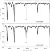 |
Fig. 4 Portion of spectra of HD 200466A (upper panel) and B (lower panel) close to Li 6708Å (thick solid line) overplotted with the synthetic spectra (thin solid lines). They are derived for: log n(Li) = 0.6, 0.8, 1.0, 1.2, 1.4, 1.6, 1.8 for HD 200466A and log n(Li) = 2.0, 2.1, 2.2, 2.3, 2.4, 2.5, 2.6 for HD 200466B. |
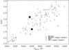 |
Fig. 5 Li abundance vs. effective temperature for the components of HD 200466A (lower black point) and B (upper black point) and stars of Hyades (640 Myr) and M67 (4 Gyr). |
3.3. Stellar age
Given the main sequence status of both components and the temperatures colder than the Sun, isochrone fitting (see above) gives inconclusive results for the ages (3.6 ± 3.4 Gyr for the primary and 3.7 ± 3.4 Gyr for the secondary). As shown in Sect. 3.2, the lithium abundance of B is similar to Hyades stars of similar temperature, while that of A is well below and similar to older stars. We then considered additional age indicators, based on magnetic activity, rotation, and kinematics.
3.3.1. X-ray emission
ROSAT identified a source (1RXS J210223.3+373856) close to HD 200466 (separation 24 arcsec with a quoted error of 33 arcsec; Voges et al. 2000). Assuming this is the X-ray counterpart of HD 200466, the X-ray luminosity derived using the calibration of Hünsch et al. (1999) is LX = 1.40 × 1028 erg/s (A+B components). Assuming similar luminosities of both components, we obtain LX = 7.0 × 1027 erg/s for the individual stars. The age resulting from the calibration by Mamajek & Hillebrand (2008) is 2.9 Gyr.
3.3.2. Chromospheric emission
The adopted SARG set-up does not include Ca II H&K in the spectral format. However, the components of HD 200466 were observed three times in 1998 with HIRES at Keck as part of the G Dwarf Planet Search (Latham 2000). We retrieved the reduced spectra from the Keck archive5.
To quantify the chromospheric emission, we built a calibration of the S index as measured in the Keck spectra and in the standard M. Wilson system. To this end we retrieved from the Keck archive several spectra of 15 stars from the list of Wright et al. (2004) in the colour range 0.72 <B − V< 0.76 and spanning various activity levels. The calibration into the standard Mt. Wilson system has a dispersion of 0.011, likely dominated by intrinsic variability of the chromospheric activity.
The values of log RHK of HD 200466A and B derived following the prescriptions of Noyes et al. (1984) and for the calculated individual B − V colours were found to be of − 4.77 and −4.69 for HD 200466A and B, respectively. The ages resulting from the calibration by Mamajek & Hillebrand (2008) are 2.8 and 1.9 Gyr for HD 200466A and B, respectively. This difference provides an estimate of the rather large uncertainties related to this method.
3.3.3. Rotational period
The only photometric time series available is that of Hipparcos. Hipparcos photometry refer to joined A+B components. The errors in the resolved photometry by Tycho are large. We analysed the individual Hipparcos photometric data, eliminating one obvious outlier and performing daily averages. The dispersion of the daily averages is 0.007 mag. The periodogram shows a peak at 20.34 days (Fig. 6), which has a false alarm probability (FAP) of 2.5% according to a bootstrap test. While not highly significant, it might represent the rotational period of one of the components. Indeed, the expected rotational period derived from the observed Ca II H&K emission using the relation by Mamajek & Hillebrand (2008) is just slightly longer (26.0 and 23.4 days for HD 200466 A and B, respectively) and the observed period is compatible with the projected rotational velocities (see below) for inclinations of about 30 and 55 deg for HD 200466A and B, respectively.
While neither the photometric nor the spectroscopic periods have confidence levels larger than 99%, the detection of a very similar period with independent techniques and at different epochs is a strong indication that indeed the rotation period of HD 200466A is about 20 d. The corresponding ages resulting from the calibration by Mamajek & Hillebrand (2008) are 2.3 and 2.1 Gyr depending on whether the 20.3 d period belongs to HD 200466A or B.
Projected rotational velocities were derived performing an FFT analysis of the CCF profiles (for all spectra involved in the line profile analysis). The procedure is described in Desidera et al. (2011). The macroturbulence was estimated from effective temperature and the B − V colours following the calibration by Valenti & Fischer (2005). We found vsiniA = 1.3 ± 0.5 km s-1 (upper limit) and vsiniB = 2.2 ± 0.8 km s-1.
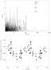 |
Fig. 6 Hipparcos photometry (joined A+B components). Upper panel: Lomb-Scargle periodogram; Lower panel: photometry phased to the best-fit period of 20.34 d. |
3.3.4. Kinematics
Absolute RV of the SARG templates of HD 200466 A and B as derived using cross-correlation with spectra of a few objects from the list of Nidever et al. (2002) lead to −8.19 ± 0.20 and −8.44 ± 0.20 km s-1, very similar to the values listed in Carney et al. (1994, −8.0 and −8.4 km s-1) and Nordstrom et al. (2004, −8.3 km s-1 from composite spectra).
We use our absolute RVs (corrected for gravitational and convective shifts as in Nidever et al. 2002) together with Hipparcos astrometry to derive space velocities and galactic orbit as in Barbieri & Gratton (2002). The space velocity is far from the regions typical of young stars (see e.g. Montes et al. 2001). Overall, the kinematics is fully compatible with an age of 2–4 Gyr.
3.3.5. Summary of stellar ages
In summary, HD 200466 is composed of two very similar components with masses slightly lower than and iron content similar to or slightly enriched with respect to the Sun. The isochrone fitting is inconclusive with regard to stellar age. From lithium, Ca II H&K emission, X-ray coronal emission, and the tentative rotational period we derived a most probable age of about 2 Gyr.
4. Radial velocity variations of HD 200466A and B
The source HD 200466A shows significant RV variability, more clearly seen after JD 2 453 800 (Fig. 7). The RV scatter (16.0 m/s) is larger than that of the companion HD 200466B (10.8 m/s) and much larger than the internal errors (4.2 m/s). As our targets are moderately active, it is important to estimate the expected RV jitter. For stars with chromospheric activity and colours like those of HD 200466 A and B, the calibration by Wright (2005) yields a median jitter of 5.9 and 7.0 m/s, with 20th percentiles of 3.9 and 4.5 m/s and 80th percentiles of 9.1 and 10.8 m/s for HD 200466 A and B, respectively. A RV jitter as high as 15 m/s, as that required to explain the RV scatter of HD 200466A, appears then very unlikely.
We consider first the secondary. It shows a small (but clearly significant) downward trend (−0.0068 ± 0.0010 m/s/d), with the root mean square (rms) of RVs decreasing from 10.8 m/s to 8.3 m/s after removing the trend (Fig. 8). This latter can be fully explained by internal errors and our estimated activity jitter (7 m/s).
The primary has larger variations, with a long-period modulation that appears more clearly in the second half of the data and a possible general upward slope. Removing the slope yields only limited reduction of rms of the RVs (13.7 m/s). The Lomb-Scargle periodogram of RVs shows a peak at about 1300 d, as well as additional power at longer periods (Fig. 7). A bootstrap test shows a FAP of 0.3% for the 1300 d peak for the original RV dataset.
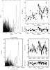 |
Fig. 7 Analysis of RVs for HD 200466A. Upper panels: measured RVs. Left panels: Lomb-Scargle periodogram. Right panels: temporal series of RVs and the residuals from the RV trend predicted by the binary orbital solution. Lower panels: RVs corrected for binary motion. Left panel: Lomb-Scargle periodogram of the residuals. Right panels: RVs of the residuals. Overplotted is the best Keplerian fit of RVs including the RV trend derived from HD 200466B and the residuals (Sect. 6). |
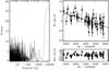 |
Fig. 8 Analysis of RVs for HD 200466B. Left panel: Lomb-Scargle periodogram. Upper right panel: temporal series of RVs. The RV trend predicted by the binary orbital solution is overplotted. Lower left panel: the residuals around this line. |
We will show in Sect. 6 that a single Keplerian orbit does not give a satisfactory fit of the RV curve. The residuals of one planet orbit show a clear long-term modulation (see Fig. 7). Including a linear RV drift in the fit yields a slope very similar to that of HD 200466B with opposite sign (+ 0.0071 ± 0.0010 m/s/d). The downward trend observed in HD 200466B and the possible upward trend in HD 200466A suggest the possibility that part of the observed RV variations are due to the binary motion of the wide pair. To further test this hypothesis we consider in Sect. 5 the constraint we can put on the binary orbit.
5. System architecture
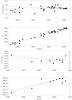 |
Fig. 9 Upper panel: relative astrometry of HD 200466. From top to bottom: projected separation vs. time; position angle (corrected for precession) vs. time; data from WDS (kindly provided by Dr. B. Mason) and from Table 2; linear fits over the whole time extent of observations are shown as solid red lines. Dotted blue lines represent the quadratic fits and dashed green lines the linear fits made separately on data taken before and after 1950.0. The dotted red line is the fit on the recent high-quality measurements, extrapolated backward in time. The lower panel displays the same quantities the first two panels, plotting only the best data (Hipparcos, speckle interferometry, adaptive optics). The dotted red line is the fit on the recent high-quality measurements, the continuous red line the linear fit over all the measurements, the dotted blue line the quadratic fit. |
We studied the orbit of the wide binary with the goal of putting constraints on the system parameters. We discuss the astrometric data and the RV difference between the components.
5.1. Astrometric data
Visual observations available in the Washington Double Star Catalog (WDS, Mason et al. 2001) were kindly provided by Dr. B. Mason (4 April 2011 version). They span the epoch from 1830 to 2007. Our TNG/AdOpt observations (Sect. 2.2) further extend the time baseline to 2008. Figure 9 shows the available measurements.
Orbital motion is clearly detected, with position angle changing from 257 to 266 deg, while the projected separation changed very little. No change in position angle and projected separation are reported in the Hipparcos catalog. We provide error bars for ρ and θ values through separate fitting data for different epochs and using the original references for some recent high-quality data (Hipparcos, speckle interferometry by Douglass et al. 1999, WDS catalog by Mason et al. 2001, CCD astrometry by Izmailov et al. 2010, and our AO data). The projected separation increases up to epoch about 1960, with a shallow decreasing slope in the last years (better seen in lower panel of Fig. 9, which shows only recent high-quality data). To estimate the significance of the curvature we performed a simulation randomly generating a dataset of 10 000 values following Gaussian distribution for each individual value of ρ and θ and their error bars to study the change in slope of the parameters in different epochs by using linear and quadratic fits. No significant curvature of the position angle trend is present and a linear fitting yields a slope of + 0.0535 ± 0.0010 deg/yr for θ. For ρ, a slope equal to −1.35 ± 0.23 mas/yr was derived using a quadratic fit at epoch 2007.0 that differs by more than 2σ from that at epoch 1850.0 (+ 2.58 ± 0.61 mas/yr). This confirms a change in slope of projected separation over time (slightly positive before 1950, slightly negative after).
There are two possible interpretations of the observed change in slope in projected separation:
-
1.
it is due to the binary motion of the wide pair (and then can be usedto constrain the orbit);
-
2.
it is due to an additional object with period of several decades (in this case, most likely the one which is responsible for the trend of RVs of HD 200466B).
The second hypothesis was rejected after the stellar activity analysis and the orbital stability analysis (see Sect. 6).
5.2. RV difference between the components
The spectra obtained with SARG allow the difference in RV difference between the components to be determined with high precision. We obtain this difference by deriving the RVs of both components using the template of HD 200466A. The similarity of the spectra of the two components ensures good quality of both RV components. The RV difference ΔRV(B − A) is of −436 m/s (at epoch 2007.0). Formal measurement errors are well below 10 m/s. True errors due to uncertainties on system velocity due to RV variability (see below), gravitational, and convective shifts, etc., likely exceed this value. We adopt 30 m/s as a conservative error bar on velocity difference.
5.3. Assuming RV trend of B due to binary orbital motion
Having obtained position and velocity on the plane of the sky and the velocity along the line of sight, a family of possible bound orbits can be obtained as a function of the unknown separation along the line of sight z. We follow the approach by Hauser et al. (1999). When assuming that the curvature in projected separation is real and due to binary orbital motion, we considered position angle, projected separation, and their derivatives with time as resulting from the linear and quadratic fits (for θ and ρ, respectively) at the reference epoch 2007.0.
Figure 10 shows the values of semi-major axis, eccentricity, periastron, and inclination for possible orbits. We obtained these values through a simulation of more than 1000 binary orbital parameter sets; we then calculated and plotted the curve that represents the mean values of random generations of the input parameters (ρ, θ, δρ/δt, δθ/δt, ΔRV, π, mA, mass ratio) for each value of z (with steps of 1 AU) with their 1σ dispersion of simulated values at each distance. Either orbits with periastron close enough to induce significant perturbations to planets around the components or very wide orbits are possible.
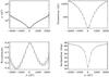 |
Fig. 10 Semi-major axis, periastron, eccentricity, and inclination of possible binary orbits as a function of the separation along the line of sight z (at reference epoch 2007.0), derived from relative positions and velocities on the plane of the sky and RV difference between the components. The probable curvature in position angle vs. time and the long-term RV trends are compatible with a limited range in z. |
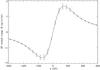 |
Fig. 11 Expected RV trend of B component at reference epoch 2007.0 as a function of z. |
To further constrain the binary orbit we considered the change in slope in the projected separation described in Sect. 5.1. The first four measurements of projected separation have ρ = 4.540 ± 0.027 arcsec and position angle θ = 257.03 ± 0.23 deg (mean epoch 1838.21). Only a limited range of values of z are compatible with these data (Fig. 12), with the projected separation providing the tightest constraints while the value of θ at 1838 epoch is compatible with a broader range of z6.
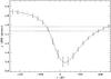 |
Fig. 12 Predicted projected separation and position angle at epoch 1840 as a function of z. The measured values and the 1σ uncertainties are overplotted as horizontal lines. |
Two groups of orbits are compatible with the astrometric data. They correspond to z ~ −150 and z ~ 400 AU. When considering the expected RV trends (for the B component), the z ~ −150 orbital solution is close to the absolute minimum of the RV trend (Fig. 11), which is only marginally lower than the observed one (−1.64 ± 0.08 vs. −2.48 ± 0.37 m/s/yr). Therefore, both the curvature in projected separation with time and the RV trend can be explained by the binary orbit and allow its full derivation.
5.4. Assuming that ρ curvature/RV trends are not due to binary orbit
The alternative hypothesis is that HD 200466B has an additional companion that is responsible for the observed RV trend.
As we have seen in Sect. 5.3, if we adopt the slope in projected separation ρ that results from the latest data, an orbital solution close to that predicting a RV trend comparable to the observations does occur. In this section, assuming an additional companion is responsible for the RV trend of HD 200466B, we consider that the observed curvature in projected separation with time is due to astrometric variations with timescales of a few decades induced by the close companion of HD 200466B responsible for the RV trend. In this case, the binary (computed using the secular projected separation trend) is marginally constrained7, with a wide family of possible orbits. Furthermore, some important parameters such as the RV difference between the components and the individual masses can be somewhat altered by the companions, adding further uncertainties.
6. First approach: a planet around A?
As discussed in Sect. 5, the most likely scenario to explain the RV, astrometric, and direct imaging data is that the RV trend of HD 200466B is due to the orbital motion of the wide pair. We will adopt the binary orbit as derived following this hypothesis. In this case, the RVs of HD 200466A should be characterized by a similar slope with opposite sign to that of HD 200466B. To analyse the RVs we then removed the expected RV trend for component A, taking into account the small mass difference between the two components. Figure 7 shows the Lomb-Scargle periodogram of the RV corrected for binary motion. The 1300 d peak becomes more prominent and isolated. The FAP for that peak derived using the bootstrap technique is 1/10 000.
Orbital fitting (after quadratically adding the estimated jitter of 7 m/s) was performed using an IDL code based on a Levenberg-Marquardt least-squares fit of RVs. The resulting orbital parameters are listed in Table 4. We considered orbits derived after correcting the RVs for the calculated binary orbit (trend 1.6 m/s/yr; Sect. 5.3) and those derived considering the opposite of the observed RV trend of HD 200466B (corrected for mass ratio between the components, 2.4 m/s/yr). The errors in the orbital parameters were derived simulating synthetic datasets taking into account the 7 m/s jitter (quadratically summed to the RV error) and performing orbital fitting for each fake RV series.
Figure 7 shows that the orbital fitting is not fully satisfactory, with residuals larger than the expected internal errors + jitter (rms = 10.5 m/s), and with some coherent structure in the first 1500 days of our observations. This calls for an in-depth study of the origin of the RV variations. In Sect. 7 we will analyse the stellar activity and reveal what we think is the true source of the RV variations.
Orbital parameters and results of Keplerian fitting for RVs.
The periodogram of the residuals shows the highest peak at 20.2 days, very close to the possible photometric period. The 20 d periodicity is more evident when considering only the data after JD 2 453 800. This is consistent with lack of coherence of rotational modulations over the whole baseline, due to finite lifetime of active regions.
The inclusion of a second planet with period about twice that of the first one might explain the unequal amplitude of the RV maxima. However, this additional planet should have a semi-major axis of about 3.6 AU, outside the critical value for orbital stability. Numerical integrations of the system orbit show that on a very short timescale the putative outer planet has an encounter with the inner one and the following evolution is chaotic. Therefore, we can safely neglect such a two–planet solution for the assumed binary orbit.
7. The true origin of the RV variations
To explain the reason for the unequal amplitude of the RV maxima we study the stellar activity and search for correlations between the RV and the BVS and measure an index on the Hα chromospheric emission. Activity induced RV variations or contamination by light from the other component are expected to produce such correlations (see e.g. Queloz et al. 2001; Martinez Fiorenzano et al. 2005), even if this diagnostic loses sensitivity for slowly rotating stars as the components of HD 200466 (see e.g. Desort et al. 2007).
The few spectra taken in poor observing conditions (seeing about 2 arcsec) do not show signatures of contamination (as expected considering the projected separation of about 4.6 arcsec) and so they were kept in the analysis. Furthermore, as the spectra of the two components were usually taken close in time and with similar observing conditions, contamination would affect in a similar way the spectra of both components. The hypothesis of contamination is not considered further.
Plots of RV vs. BVS correlation of HD 200466 A and B are shown in Figs. 13 and 14, along with the Lomb-Scargle periodograms of the BVS; this show a marginal correlation with the original (i.e. uncorrected for binary motion) RVs of HD 200466A (Pearson correlation coefficient of 0.33 and Spearman rank correlation 0.25, with probability of occurring by chance of <0.5 and 3.7%, respectively). The correlation is weaker for the RVs corrected for binary motion (probability 20%). Lomb-Scargle periodograms show some power close to the RV period, but of low significance. One of the highest peaks at short periods is very close to the 20 d periods seen in the Hipparcos photometric time series (Sect. 3.3.3) and RV residuals from Keplerian orbit (see Sect. 6). A similar analysis for the B component yields a highest peak at about 30 d.
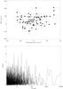 |
Fig. 13 Upper panel: BVS vs. RV (corrected for trend) for HD 200466A. Lower panel: Lomb-Scargle periodogram of BVS of HD 200466A. The two vertical dotted lines mark the periods seen in the RV time series (1300 d) and in the residuals from Keplerian orbit (20.25 days). |
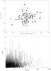 |
Fig. 14 Upper panel: BVS vs. RV (corrected for trend) for HD 200466B. Lower panel: Lomb-Scargle periodogram of BVS of HD 200466B. The vertical dotted line marks the period seen in the RV time series of HD 200466A (1300 d). |
Of course, the 1300 d period is very different from the rotational period of the star, which is most likely close to 20 days. It might instead be a magnetic activity cycle, characterized by a higher amplitude in the last years of our observations than in the first half.
In Fig. 15 the Hα index of HD 200466A correlates with the RV, indicating that the stellar activity could be responsible for the RVs variations. In particular in Fig. 16 we show the time dependence of the activity index compared with the RV time series. The two plots look very similar to each other. This is a clear signature of the large variation of the activity of HD 200466A. We also measured the activity index for HD 200466B (see Fig. 17); in this case there is no signature at long periods; the strongest peak in the periodogram is at 12.7 d. However, the S/N of this detection is low (2.7), so that this result has a low confidence level.
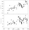 |
Fig. 16 Hα vs. JD and RV time series for HD 200466A. The modulation of the RV variations is due to the stellar activity cycle. |
In summary, although there is not a highly significant correlation between RVs and line bisectors, there is a clear indication of activity from the correlation between RVs and Hα line core strength. We argue that the RV variations observed in the primary component is related to the stellar activity cycle.
We also note that the relation between rotational period and length of the activity cycle has been discussed by several authors (see e.g. Baliunas et al. 1996; Olah et al. 2009) because it provides useful information on the dynamo mechanism (Durney & Stenflo 1972). If we compare our results for HD 200466A with those for other stars (see Fig. 5 of Olah et al. 2009), we find that this star falls in a well populated region of this diagram close to the relation for “shortest cycle lengths”; a similar result is obtained considering data from Lovis et al. (2011). In addition, a long-term trend is clearly present in our activity measures. It suggests that additional longer cycles should be present, which is a common finding for solar-type stars (see Baliunas et al. 1996; and Olah et al. 2009). On the other hand, the lack of a detectable cycle in HD 200466B is not at all anomalous; Lovis et al. (2011) detected cycles only in about a third of the FGK stars with activity levels similar to those of HD 200466A and B.
8. A corrected radial velocity series for HD 200466A
Lovis et al. (2011) proposed two different approaches to correct RVs for the signal due to the activity cycle, and Dumusque et al. (2011) showed how the signal due to planets can be extracted when such corrections are included in the data analysis. We explored such approaches for the case of HD 200466A. The basic idea is that long-term activity should be positively correlated with RVs, essentially because magnetic fields related to activity inhibit convection and then reduce the blueshift of spectral lines due to the ascending hot bubbles in the subatmospheric convection zones. At a first approximation, we expect that the RV signal should then be corrected for a factor which is proportional to the activity level, as measured by the emission in the Hα core. The conversion factor may be derived empirically by fitting the RV curve vs. Hα. There is only one free parameter to be determined.
A periodogram analysis of the time series for the Hα index gives a period of 1413 ± 38 d and an amplitude of 0.0155 ± 0.014. Following Dumusque et al. (2011), we then fitted the RV curve for HD 200466A with a sinusoid having the same period and phase of the solution found for the Hα index, after having subtracted a linear trend corresponding to the binary orbital motion. The best fit is obtained for an amplitude of 10.5 m/s. Subtraction of this signal reduces the rms scatter of the RVs from 15.9 m/s down to 11.6 m/s.
A periodogram analysis of these corrected RVs does not yield a single dominant peak. The strongest peak is at a period of 20.241 ± 0.012 d with an amplitude of 8.3 ± 1.6 m/s; it coincides with the photometric signal obtained from the Hipparcos data (see Sect. 3.1) that is also present in the periodogram of the bisectors (see Sect. 7) and can be interpreted as the rotational period of the star. Inclusion of this signal reduces the rms scatter of the RVs down to 10.2 m/s.
Once a sinusoid corresponding to this peak is subtracted, the three next highest peaks are at periods of 27.918 ± 0.014 d, 1102.24 ± 0.016 d, and 2702 ± 30 d. While we deem the rotational period to be quite robust, because it is present in completely independent time series, although never at a high level of significance, the remaining peaks are not robust; their frequencies change if, for instance, we drop the last four points of the time series.
A similar approach has been criticized by Meunier & Lagrange (2013) because it neglects the fact that activity and RV variations may be not sinusoidal with time. They then suggested adopting a linear relation between the activity indicator (in our case, the Hα index) and the RVs, and then removing such a trend. We applied a correction obtained by averaging the two results obtained using RV and Hα index as independent variables. The corrected RVs have a very strong trend with time, with a slope of −0.0117 m/s/day. This is a consequence of the presence of a quite strong trend of the Hα index with time, while RVs only have a more modest trend. A Fourier analysis of the residuals along this linear trend has the three highest peaks at 1145, 5.47, and 19.36 d. The first peak resembles the long period that we attribute to activity, possibly signalling that the correction to be applied is more complex than a simple linear function. The third period is possibly related to the power at about 20 d that we attribute to rotation.
9. Discussion and conclusion
9.1. Lithium difference between stars with and without planets?
It is well know that lithium abundances in old solar-type stars show a large scatter, both in clusters and field (e.g. Pasquini et al. 1997, for the open cluster M67). Large differences were also reported in a few cases of wide binaries with similar components (King et al. 1997; and Martin et al. 2002). The star HD 200466 is a rather extreme case in this context, because of the large difference in lithium levels between the components (by a factor of at least 9) and because the difference is in the opposite direction with respect to the usual pattern of lower lithium content toward lower temperatures, and therefore should have a different origin. The very small errors in the temperature difference (53 ± 23 K) makes this result very robust.
In the past few years, there were several attempts to correlate such variations with the presence of planets, with indications that stars with planets typically have lower lithium abundance while some other works reached the opposite conclusion (see Gonzalez 2006, for a summary and references). The work by Israelian et al. (2009) supports the reality of such a correlation and theoretical models have been developed to explain these results. It is possible that a slow stellar rotation resulting from a longer star-disk interaction phase affects the core-envelope coupling. This might produce a stronger differential rotation at the base of the convective envelope and then larger lithium depletion in slow rotators (Bouvier 2008). Castro et al. (2009) considered instead the possible role of angular momentum transfer due to planetary migration.
The components of HD 200466 are slightly cooler than the limits of the sample considered in Israelian et al. (2009). We do not have an indication of the presence of giant planets within a few AU. The difference in the activity cycle is the other peculiar feature of HD 200466, so one may think about a possible link between Li abundances and stellar activity. However, a comparison of the Li abundances (from Sousa et al. 2010) in stars with and without activity cycles (from Lovis et al. 2011) does not show any correlation between these two quantities, likely because activity is variable on a large range of timescales and detection of cycles in given stars might be related to the epoch of observation. A systematic investigation of the characteristics of the activity cycles in multiple systems with similar components and the possible correlations of the activity parameters with other stellar properties is postponed to a forthcoming work.
9.2. Conclusion
The long-term RV trends of both components have opposite slopes and similar amplitudes. This fact suggests that we are observing the binary motion, and the available astrometric measurements as well as the non-detection of additional close companions in our adaptive optics images support this scenario. Strong constraints are put on the orbital solution of the binary, which is very eccentric and with a periastron as small as 22 AU, limiting the zone for dynamical stability around HD 200466 to slightly more than 3 AU.
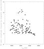 |
Fig. 18 Adapted from Lovis et al. (2011). Effective impact of magnetic cycles on RV for HARPS sample stars with a detected cycle, shown as a function of Teff. The location of HD 200466A in this diagram is shown as an open star. |
A vigorous activity cycle is present in HD 200466A during the second half of the observing range. This phenomenon mimics the presence of a planetary system with a period of 1300 d. As the star is moderately young (about 2 Gyr) and active (expected RV jitter about 5.9 m/s), the possibility of activity-induced jitter was considered. We did not detect a strong correlation between RV and BVS, while the Hα analysis leads a different conclusion. The star HD 200466A shows a cycle amplitude as high as the maximum ones seen in the HARPS sample (see Fig. 18 adapted from Lovis et al. 2011). The jitter value is higher than the one predicted by Wright (2005) for HD 200466A (5.9 m/s).
The residuals from a sinusoidal fit with period and phase set by the Hα observations show the highest peak at about 20 d, very close to the probable (FAP = 2.5%) photometric period derived from the Hipparcos photometry. This may be interpreted as the rotational period of the star.
We conclude this paper by stressing the importance of distinguishing between the activity cycles and planetary signatures. We studied the stellar activity of HD 200466A and estimated that the cycle semi-amplitude could amount to levels up to >10 m/s, with rather large variations from one cycle to another. Therefore, the monitoring of activity indicators is necessary in order to solve the true origin of the RV variations, whether they are due to a planet or to the stellar activity.
Online material
This is further evidence against the presence of additional bright stellar components in the system.
If we considered the phase and length of the activity cycle discussed in Sect. 7, these spectra were taken close to a maximum in the activity cycle. However, activity data also show a long-term trend that, if extrapolated at the epoch of these observations, indicates an activity level well below the average of our observation.
These conclusions change only marginally if we consider a more extended data set to constrain the separation at early phases, e.g. the first eight data points before epoch 1868.
Only the values of z close to 0 are excluded because they would imply a position angle different from that observed.
Acknowledgments
This research has made use of the SIMBAD database, operated at the CDS, Strasbourg, France. This research has made use of the Washington Double Star Catalog maintained at the US Naval Observatory. This research has made use of the Keck Observatory Archive (KOA), which is operated by the W. M. Keck Observatory and the NASA Exoplanet Science Institute (NExScI), under contract with the National Aeronautics and Space Administration. We thank the TNG staff for contributing to the observations and the TNG TAC for the generous allocation of observing time. We thank R. Ragazzoni and A. Ghedina for useful discussions on TNG/AdOpt. We thank B. Mason for providing the astrometric data collected in the Washington Double Star Catalog. This work was partially funded by PRIN-INAF 2008 “Environmental effects in the formation and evolution of extrasolar planetary systems”. E.C. acknowledges support from CARIPARO. We warmly thank the anonymous referee for her/his careful reading and detailed comments to the manuscript.
References
- Baliunas, S. L., Nesme-Ribes, E., Sokoloff, D., & Soon, W. 1996, ApJ, 460, 848 [NASA ADS] [CrossRef] [Google Scholar]
- Baraffe, I., Chabrier, G., Barman, T. S., Allard, F., & Hauschildt, P. H. 2003, A&A, 402, 701 [NASA ADS] [CrossRef] [EDP Sciences] [Google Scholar]
- Barbieri, M., & Gratton, R. 2002, A&A 384, 879 [NASA ADS] [CrossRef] [EDP Sciences] [Google Scholar]
- Boisse, I., Bouchy, F., Hébrard, G., et al. 2011, A&A, 528, A4 [NASA ADS] [CrossRef] [EDP Sciences] [Google Scholar]
- Bouvier, J. 2008, A&A, 489, L53 [NASA ADS] [CrossRef] [EDP Sciences] [Google Scholar]
- Carney, B. W., Latham, D. W., Laird, J. B., & Aguilar, L. A. 1994, AJ, 107, 2240 [NASA ADS] [CrossRef] [Google Scholar]
- Carolo, E. 2012, Ph.D. Thesis, Un. Padova, Italy [Google Scholar]
- Castro, M., Vauclair, S., Richard, O., & Santos, N. C. 2009, A&A, 494, 663 [NASA ADS] [CrossRef] [EDP Sciences] [Google Scholar]
- Cecconi, M., Ghedina, A., Bagnara, P., et al. 2006, Proc. SPIE, 6272, 2G [Google Scholar]
- Chabrier, G., Baraffe, I., Allard, F., & Hauschildt, P. 2000, ApJ, 542, 464 [NASA ADS] [CrossRef] [Google Scholar]
- Cincunegui, C., Díaz, R. F., & Mauas, P. J. D. 2007, A&A, 476, 309 [CrossRef] [EDP Sciences] [Google Scholar]
- da Silva, L., Girardi, L., Pasquini, L., et al. 2006, A&A, 458, 609 [NASA ADS] [CrossRef] [EDP Sciences] [Google Scholar]
- Delfosse, X., Forveille, T., Segransan, D., et al. 2000, A&A, 364, 217 [NASA ADS] [Google Scholar]
- Desidera, S., Gratton, R. G., Scuderi, S., et al. 2004, A&A, 420, 683 [NASA ADS] [CrossRef] [EDP Sciences] [Google Scholar]
- Desidera, S., Gratton, R. G., Endl, M., et al. 2010 in Planets in Binary Star Systems (Berlin: Springer), Astrophys. Space Sci. Lib., 366, 105 [Google Scholar]
- Desidera, S., Carolo, E., Gratton, R. G., et al. 2011, A&A, 533, A90 [NASA ADS] [CrossRef] [EDP Sciences] [Google Scholar]
- Desort, M., Lagrange, A.-M., Galland, F., Udry, S., & Mayor, M. 2007, A&A, 473, 983 [NASA ADS] [CrossRef] [EDP Sciences] [Google Scholar]
- Douglass, G. G., Mason, B. D., Germain, M. E., & Worley, C. E. 1999, AJ, 118, 1395 [NASA ADS] [CrossRef] [Google Scholar]
- Dravins, D. 1992, Proc. ESO Workshop on High Resolution Spectroscopy with the VLT, ed. M.-H. Ulrich, 55 [Google Scholar]
- Dumusque, X., Lovis, C., Ségransan, D., et al. 2011, A&A, 535, A55 [NASA ADS] [CrossRef] [EDP Sciences] [Google Scholar]
- Durney, B. R., & Stenflo, J. O. 1972, Ap&SS, 15, 307 [NASA ADS] [CrossRef] [Google Scholar]
- Endl, M., Kürster, M., & Els, S. 2000, A&A, 362, 585 [Google Scholar]
- ESA 1997, The Hipparcos and Tycho Catalogues, ESA SP-1200 [Google Scholar]
- Figueira, P., Marmier, M., Bonfils, X., et al. 2010, A&A, 513, L8 [NASA ADS] [CrossRef] [EDP Sciences] [Google Scholar]
- Gomes da Silva, J., Santos, N. C., Bonfils, X., et al. 2011, A&A, 534, A30 [NASA ADS] [CrossRef] [EDP Sciences] [Google Scholar]
- Gonzalez, G. 2006, PASP, 118, 1494 [NASA ADS] [CrossRef] [Google Scholar]
- Gratton, R. G., Bonanno, G., Bruno, P., et al. 2001, Exp. Astron., 12, 107 [NASA ADS] [CrossRef] [Google Scholar]
- Hatzes, A. P. 2002, Astron. Nachr., 323, 392 [NASA ADS] [CrossRef] [Google Scholar]
- Hatzes, A. P., & Cochran, W. D. 1998, MNRAS, 293, 469 [NASA ADS] [CrossRef] [Google Scholar]
- Hauser, H. M., & Marcy, G. W. 1999, PASP, 111, 321 [NASA ADS] [CrossRef] [Google Scholar]
- Hernan-Obispo, M., Galvez-Ortiz, M. C., Anglada-Escude, G., et al. 2010, A&A, 512, A45 [NASA ADS] [CrossRef] [EDP Sciences] [Google Scholar]
- Huelamo, N., Figueira, P., Bonfils, X., et al. 2008, A&A, 489, L9 [NASA ADS] [CrossRef] [EDP Sciences] [Google Scholar]
- Hünsch, M., Schmitt, J. H. M. M., Sterzik, M. F., & Voges, W. 1999, A&AS, 135, 319 [NASA ADS] [CrossRef] [EDP Sciences] [Google Scholar]
- Isaacson, H., & Fischer, D. 2010, ApJ, 725, 875 [NASA ADS] [CrossRef] [Google Scholar]
- Israelian, G., Delgado Mena, E., Santos, N. C., et al. 2009, Nature, 462, 189 [NASA ADS] [CrossRef] [PubMed] [Google Scholar]
- Izmailov, I. S., Khovricheva, M. L., Khovrichev, M. Y., et al. 2010, Astron. Lett., 36, 349 (Pisma Astron. Zhur. 36, 365, 2010) [NASA ADS] [CrossRef] [Google Scholar]
- King, J. R., Deliyannis, C. P., Hiltgen, D. D., et al. 1997, AJ, 113, 1871 [NASA ADS] [CrossRef] [Google Scholar]
- Lanza, A. F., Boisse, I., Bouchy, F., Bonomo, A. S., & Moutou, C. 2011, A&A, 533, A44 [NASA ADS] [CrossRef] [EDP Sciences] [Google Scholar]
- Latham, D. 2000, in Disks, Planetesimals, and Planets, eds. F. Garzon, C. Eiroa, D. de Winter, & T. J. Mahoney, ASP Conf. Proc., 219, 596 [Google Scholar]
- Lovis, C., Dumusque, X., Santos, N. C., et al. 2011, A&A, submitted [arXiv:1107.5325] [Google Scholar]
- Martin, E. L., Basri, G., Pavlenko, Y., & Lyubchik, Y. 2002, ApJ, 579, 437 [NASA ADS] [CrossRef] [Google Scholar]
- Mason, B. D., Wycoff, G. L., Hartkopf, W. I., Douglass, G. G., & Worley, C. E. 2001, AJ, 122, 3466 [Google Scholar]
- Mamajek, E. E., & Hillenbrand, L. A. 2008, ApJ, 687, 1264 [NASA ADS] [CrossRef] [Google Scholar]
- Martínez Fiorenzano, A. F., Gratton, R. G., Desidera, S., Cosentino, R., & Endl, M. 2005, A&A, 442, 775 [NASA ADS] [CrossRef] [EDP Sciences] [Google Scholar]
- Meunier, N., & Delfosse, X. 2009, A&A, 501, 1103 [NASA ADS] [CrossRef] [EDP Sciences] [Google Scholar]
- Meunier, N., & Lagrange, A. M. 2013, A&A, 551, A101 [NASA ADS] [CrossRef] [EDP Sciences] [Google Scholar]
- Meunier, N., Desort, M., & Lagrange, A. M. 2010, A&A, 512, A39 [NASA ADS] [CrossRef] [EDP Sciences] [Google Scholar]
- Montes, D., Lopez-Santiago, J., Galvez, M. C., et al. 2001, MNRAS, 328, 45 [NASA ADS] [CrossRef] [MathSciNet] [Google Scholar]
- Nassau, J. J., & Stephenson, C. B. 1961, ApJ, 133, 920 [NASA ADS] [CrossRef] [Google Scholar]
- Nidever, D. L., Marcy, G. W., Butler, R. P., Fischer, D. A., & Vogt, S. S. 2002, ApJS, 141, 503 [NASA ADS] [CrossRef] [Google Scholar]
- Nordstrom, B., Mayor, M., Andersen, J., et al. 2004, A&A, 418, 989 [NASA ADS] [CrossRef] [EDP Sciences] [Google Scholar]
- Noyes, R. W., Hartmann, L. W., Baliunas, S. L., Duncan, D. K., & Vaughan, A. H. 1984, ApJ, 279, 763 [NASA ADS] [CrossRef] [Google Scholar]
- Oláh, K., Kollatáth, Z., Granzer, T., et al. 2009, A&A, 501, 703 [NASA ADS] [CrossRef] [EDP Sciences] [Google Scholar]
- Pasquini, L., Randich, S., & Pallavicini, R. 1997 A&A, 325, 535 [NASA ADS] [Google Scholar]
- Paulson, D. B., Saar, S. H., Cochran, W. D., & Henry, G. W. 2004, AJ, 127, 1644 [NASA ADS] [CrossRef] [Google Scholar]
- Queloz, D., Henry, G. W., Sivan, J. P., et al. 2001, A&A, 379, 279 [NASA ADS] [CrossRef] [EDP Sciences] [Google Scholar]
- Saar, S. H., & Donahue, R. A. 1997, ApJ, 485, 319 [NASA ADS] [CrossRef] [Google Scholar]
- Saar, S. H., & Fischer, R. A. 2000, ApJ, 534, L105 [NASA ADS] [CrossRef] [PubMed] [Google Scholar]
- Setiawan, J., Henning, Th., Launhardt, R., et al. 2008, Nature, 451, 38 [NASA ADS] [CrossRef] [PubMed] [Google Scholar]
- Skrutskie, M. F., Cutri, R. M., Stiening, R., et al. 2006, AJ, 131, 1163 [NASA ADS] [CrossRef] [Google Scholar]
- Sousa, S. G., Fernandes, J., Israelian, G., & Santos, N. C. 2010, A&A, 512, L5 [NASA ADS] [CrossRef] [EDP Sciences] [Google Scholar]
- Torres, G., Konacki, M., Sasselov, D. D., & Jha, S. 2004, ApJ, 614, 979 [NASA ADS] [CrossRef] [Google Scholar]
- Van Leuveen, F. 2007n A&A, 474, 653 [NASA ADS] [CrossRef] [EDP Sciences] [Google Scholar]
- Valenti, J., & Fischer, D. 2005, ApJS, 159, 141 [NASA ADS] [CrossRef] [MathSciNet] [Google Scholar]
- Voges, W., Aschenbach, B., Boller, Th., et al. 2000, ROSAT All-Sky Survey Faint Source Catalog, VizieR Online Data Catalogue: IX/29 [Google Scholar]
- Wright, J. T. 2005, PASP, 117, 657 [NASA ADS] [CrossRef] [Google Scholar]
- Wright, J. T., Marcy, G. W., Butler, R. P, & Vogt, S. S. 2004, ApJS, 152, 261 [NASA ADS] [CrossRef] [Google Scholar]
All Tables
All Figures
|
Fig. 1 Hα profile of a sample of 30 spectra of HD 200466A. The dotted lines correspond to the two ranges used to calculate the normalized continuum. The solid line corresponds to the “on line” band used for the activity analysis. |
| In the text | |
|
Fig. 2 Residuals on the composite TNG/AdOpt image after subtraction of the two components of the HD 200466 system. |
| In the text | |
|
Fig. 3 Detection limits from TNG/AdOpt images of HD 200466. The contrast in the Brγ band is shown as a function of projected separation in arcsec and AU. Corresponding values of mass limits are shown. |
| In the text | |
|
Fig. 4 Portion of spectra of HD 200466A (upper panel) and B (lower panel) close to Li 6708Å (thick solid line) overplotted with the synthetic spectra (thin solid lines). They are derived for: log n(Li) = 0.6, 0.8, 1.0, 1.2, 1.4, 1.6, 1.8 for HD 200466A and log n(Li) = 2.0, 2.1, 2.2, 2.3, 2.4, 2.5, 2.6 for HD 200466B. |
| In the text | |
|
Fig. 5 Li abundance vs. effective temperature for the components of HD 200466A (lower black point) and B (upper black point) and stars of Hyades (640 Myr) and M67 (4 Gyr). |
| In the text | |
|
Fig. 6 Hipparcos photometry (joined A+B components). Upper panel: Lomb-Scargle periodogram; Lower panel: photometry phased to the best-fit period of 20.34 d. |
| In the text | |
|
Fig. 7 Analysis of RVs for HD 200466A. Upper panels: measured RVs. Left panels: Lomb-Scargle periodogram. Right panels: temporal series of RVs and the residuals from the RV trend predicted by the binary orbital solution. Lower panels: RVs corrected for binary motion. Left panel: Lomb-Scargle periodogram of the residuals. Right panels: RVs of the residuals. Overplotted is the best Keplerian fit of RVs including the RV trend derived from HD 200466B and the residuals (Sect. 6). |
| In the text | |
|
Fig. 8 Analysis of RVs for HD 200466B. Left panel: Lomb-Scargle periodogram. Upper right panel: temporal series of RVs. The RV trend predicted by the binary orbital solution is overplotted. Lower left panel: the residuals around this line. |
| In the text | |
|
Fig. 9 Upper panel: relative astrometry of HD 200466. From top to bottom: projected separation vs. time; position angle (corrected for precession) vs. time; data from WDS (kindly provided by Dr. B. Mason) and from Table 2; linear fits over the whole time extent of observations are shown as solid red lines. Dotted blue lines represent the quadratic fits and dashed green lines the linear fits made separately on data taken before and after 1950.0. The dotted red line is the fit on the recent high-quality measurements, extrapolated backward in time. The lower panel displays the same quantities the first two panels, plotting only the best data (Hipparcos, speckle interferometry, adaptive optics). The dotted red line is the fit on the recent high-quality measurements, the continuous red line the linear fit over all the measurements, the dotted blue line the quadratic fit. |
| In the text | |
|
Fig. 10 Semi-major axis, periastron, eccentricity, and inclination of possible binary orbits as a function of the separation along the line of sight z (at reference epoch 2007.0), derived from relative positions and velocities on the plane of the sky and RV difference between the components. The probable curvature in position angle vs. time and the long-term RV trends are compatible with a limited range in z. |
| In the text | |
|
Fig. 11 Expected RV trend of B component at reference epoch 2007.0 as a function of z. |
| In the text | |
|
Fig. 12 Predicted projected separation and position angle at epoch 1840 as a function of z. The measured values and the 1σ uncertainties are overplotted as horizontal lines. |
| In the text | |
|
Fig. 13 Upper panel: BVS vs. RV (corrected for trend) for HD 200466A. Lower panel: Lomb-Scargle periodogram of BVS of HD 200466A. The two vertical dotted lines mark the periods seen in the RV time series (1300 d) and in the residuals from Keplerian orbit (20.25 days). |
| In the text | |
|
Fig. 14 Upper panel: BVS vs. RV (corrected for trend) for HD 200466B. Lower panel: Lomb-Scargle periodogram of BVS of HD 200466B. The vertical dotted line marks the period seen in the RV time series of HD 200466A (1300 d). |
| In the text | |
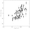 |
Fig. 15 RV–Hα correlation for HD 200466A. |
| In the text | |
|
Fig. 16 Hα vs. JD and RV time series for HD 200466A. The modulation of the RV variations is due to the stellar activity cycle. |
| In the text | |
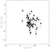 |
Fig. 17 HD 200466B RV–Hα correlation. |
| In the text | |
|
Fig. 18 Adapted from Lovis et al. (2011). Effective impact of magnetic cycles on RV for HARPS sample stars with a detected cycle, shown as a function of Teff. The location of HD 200466A in this diagram is shown as an open star. |
| In the text | |
Current usage metrics show cumulative count of Article Views (full-text article views including HTML views, PDF and ePub downloads, according to the available data) and Abstracts Views on Vision4Press platform.
Data correspond to usage on the plateform after 2015. The current usage metrics is available 48-96 hours after online publication and is updated daily on week days.
Initial download of the metrics may take a while.