| Issue |
A&A
Volume 566, June 2014
|
|
|---|---|---|
| Article Number | A126 | |
| Number of page(s) | 19 | |
| Section | Planets and planetary systems | |
| DOI | https://doi.org/10.1051/0004-6361/201323084 | |
| Published online | 23 June 2014 | |
Search for cool giant exoplanets around young and nearby stars
VLT/NaCo near-infrared phase-coronagraphic and differential imaging⋆
1 LUTH, Observatoire de Paris, CNRS and University Denis Diderot Paris 7, 5 place Jules Janssen, 92195 Meudon, France
2 INAF – Osservatorio Astronomico di Padova, Vicolo dell’Osservatorio 5, 35122 Padova, Italy
e-mail: This email address is being protected from spambots. You need JavaScript enabled to view it.
3 LESIA, Observatoire de Paris, CNRS, University Pierre et Marie Curie Paris 6 and University Denis Diderot Paris 7, 5 place Jules Janssen, 92195 Meudon, France
4 IPAG, Université Joseph Fourier, CNRS, BP 53, 38041 Grenoble, France
5 Max-Planck-Institut für Astronomie, Königstuhl 17, 69117 Heidelberg, Germany
Received: 19 November 2013
Accepted: 12 April 2014
Abstract
Context. Spectral differential imaging (SDI) is part of the observing strategy of current and future high-contrast imaging instruments. It aims to reduce the stellar speckles that prevent the detection of cool planets by using in/out methane-band images. It attenuates the signature of off-axis companions to the star, such as angular differential imaging (ADI). However, this attenuation depends on the spectral properties of the low-mass companions we are searching for. The implications of this particularity on estimating the detection limits have been poorly explored so far.
Aims. We perform an imaging survey to search for cool (Teff< 1000–1300 K) giant planets at separations as close as 5–10 AU. We also aim to assess the sensitivity limits in SDI data taking the photometric bias into account. This will lead to a better view of the SDI performance.
Methods. We observed a selected sample of 16 stars (age <200 Myr, distance <25 pc) with the phase-mask coronagraph, SDI, and ADI modes of VLT/NaCo.
Results. We do not detect any companions. As for the estimation of the sensitivity limits, we argue that the SDI residual noise cannot be converted into mass limits because it represents a differential flux, unlike what is done for single-band images, in which fluxes are measured. This results in degeneracies for the mass limits, which may be removed with the use of single-band constraints. We instead employ a method of directly determining the mass limits and compare the results from a combined processing SDI-ADI (ASDI) and ADI. The SDI flux ratio of a planet is the critical parameter for the ASDI performance at close-in separations (≲1′′). The survey is sensitive to cool giant planets beyond 10 AU for 65% and 30 AU for 100% of the sample.
Conclusions. For close-in separations, the optimal regime for SDI corresponds to SDI flux ratios higher than ~2. According to the BT-Settl model, this translates into Teff ≲ 800 K, which is significantly lower than the methane condensation temperature (~1300 K). The methods described here can be applied to the data interpretation of SPHERE. In particular, we expect better performance with the dual-band imager IRDIS, thanks to more suitable filter characteristics and better image quality.
Key words: planetary systems / instrumentation: adaptive optics / methods: observational / methods: data analysis / techniques: high angular resolution / techniques: image processing
Based on observations collected at the European Southern Observatory, Chile, ESO programs 085.C-0257A, 086.C-0164A, and 088.C-0893A.
© ESO, 2014
1. Introduction
The search for exoplanets by direct imaging is challenged by very large brightness ratios between stars and planets at short angular separations. Current facilities on large ground-based telescopes or in space allow adequate contrasts to be reached, and have revealed a few planetary-mass objects (Marois et al. 2008; Marois et al. 2010; Lagrange et al. 2009; Rameau et al. 2013b; Kuzuhara et al. 2013) either massive (>3 Jupiter masses or MJ) and young (<100–200 Myr) or with large angular separations (>1′′). Even though some of them are questioned (Kalas et al. 2008), these objects very likely represent the top of the giant planet population at long periods. They are therefore very important for understanding the planet’s formation mechanisms. These discoveries have been favored by longstanding instrumental developments such as adaptive optics (AO) and coronagraphy, but also by dedicated observing strategies and post-processing methods like differential imaging.
The purpose of differential imaging is to attenuate the stellar speckles which prevent the detection of faint planets around the star. More precisely, a reference image of the star is built and subtracted from the science images. Several kinds of differential imaging have been proposed in the past decade. Angular differential imaging (ADI) takes advantage of the field rotation occurring in an alt-az telescope (Marois et al. 2006a). Spectral differential imaging (SDI) exploits the natural wavelength dependence of a star image (Racine et al. 1999). An extension of this technique consists in using the spectral information in many spectral channels, provided for instance by an integral field spectrometer (Sparks & Ford 2002; Thatte et al. 2007; Crepp et al. 2011; Pueyo et al. 2012). Polarimetric differential imaging uses differences between the polarimetric fluxes of the star and the planet or disk (Kuhn et al. 2001), but has not permitted any planet detections so far. Introducing a difference between star and planet properties allows differentiating the unwanted stellar speckles from the much fainter planet signals. Still, achieving high performance with these methods also requires good knowledge of the instrument behavior and biases.
Large direct imaging surveys have tentatively constrained the frequency of young giant planets at long periods (≳10–20 AU) to ~10–20% (e.g., Lafrenière et al. 2007; Chauvin et al. 2010; Vigan et al. 2012; Rameau et al. 2013a; Wahhaj et al. 2013a; Nielsen et al. 2013; Biller et al. 2013). Typical contrasts of 10 to 15 mag have been obtained, but for separations beyond ~1′′. Consequently, the occurrence of young giant planets down to a few Jupiter masses was mostly investigated at physical separations from ~10 AU to hundreds of AU, β Pictoris b being the object detected with the closest separation (8 AU, Lagrange et al. 2010). To analyze closer-in, colder, and less-massive giant planets, we need to push the contrast performance further. For this very purpose, several new-generation imaging instruments are now ready to start operation, such as SPHERE (Spectro-Polarimetric High-contrast Exoplanet REsearch, Beuzit et al. 2008) and GPI (Gemini Planet Imager, Macintosh et al. 2008). They were built to take advantage of several high-contrast imaging techniques, namely extreme AO, advanced coronagraphy, ADI, and SDI.
The evolutionary models extrapolated from stellar mechanisms (Burrows et al. 1997; Chabrier et al. 2000) predict that Jovian planets are very hot when formed; they cool over time and can be relatively bright at young ages1. SDI (Racine et al. 1999) is intended to take advantage of the presence of a methane absorption band at ~1.6 μm in the spectra of cool (≲1300 K) giant planets (Burrows et al. 1997; Chabrier et al. 2000), while the star is not expected to contain this chemical element. Thus, this spectral feature provides an efficient tool for disentangling stellar speckles from planet signal(s). SDI offers the potential to reach the detection of planets with lower masses than those already discovered by direct imaging. However, spectroscopic observations of a few young giant planets have only shown weak absorption by methane in the H band, which could be explained by the low surface gravity of these objects (Barman et al. 2011a,b; Oppenheimer et al. 2013; Konopacky et al. 2013).
In practice, SDI also produces a significant attenuation of the planet itself, because the latter is present in the reference image used for the speckle subtraction. This attenuation has to be quantified to derive its photometry accurately. To date, only two independent surveys have been made using SDI with the Very Large Telescope (VLT), as well as with the Multiple Mirror Telescope (MMT) (Biller et al. 2007) and the Gemini South telescope (Biller et al. 2013; Nielsen et al. 2013; Wahhaj et al. 2013a), but they have not reported any detections of planetary-mass objects yet. The non-detection results were exploited to assess the frequency of giant planets at long periods. Nielsen et al. (2008) did not consider the biases introduced by SDI for their analysis, unlike Biller et al. (2013), Nielsen et al. (2013), and Wahhaj et al. (2013a) for the statistical analysis of the NICI Campaign.
The observing strategy of the NICI Campaign is based on the complementarity of two observing modes in order to optimize the survey sensitivity: ADI (Marois et al. 2006a) and the combination of SDI and ADI (ASDI). These two observing modes are not performed simultaneously on the same target, because the spectral filters used are different (large-band and narrow-band, respectively). The ADI and ASDI contrast curves presented in Biller et al. (2013), Nielsen et al. (2013), and Wahhaj et al. (2013a) are corrected from the attenuation and the artifacts produced by the reduction pipeline except for the SDI part (for the ASDI curves), because the attenuation depends on the spectral properties of a planet. Nevertheless, this point is taken into account for the planet frequency study. Both ADI and ASDI contrast curves are considered in this analysis, but only the best detection limit is finally used. The results are essentially consistent with the previous surveys.
We note that Biller et al. (2013) and Nielsen et al. (2013) do not report any ASDI mass detection limits for individual targets, because of the particularities of the SDI attenuation. Wahhaj et al. (2013a) present individual mass detection limits combining ADI and ASDI, using the contrast–mass conversion based on evolutionary models. We argue in this work that this method is inadequate for interpreting the dual-band imaging data analyzed with SDI-based algorithms. Our arguments are also relevant to IFS data processed with similar techniques (Sparks & Ford 2002; Crepp et al. 2011; Pueyo et al. 2012).
In this paper, we present the outcome of a small survey of 16 stars performed with NaCo (Nasmyth Adaptive Optics System and Near-Infrared Imager and Spectrograph), the near-IR AO-assisted camera of the VLT (Rousset et al. 2003; Lenzen et al. 2003). Our prime objective is to observe a selected sample of young (≲200 Myr) and nearby (≲25 pc) stars to search for massive but cool gas giant planets at separations as small as 5–10 AU. For this purpose, we combine state-of-the-art high-contrast imaging techniques similar to those implemented in SPHERE (Beuzit et al. 2008). Our second objective is to address the problem of assessing detection limits in SDI data, which is important when it falls to very short angular separations (<0.5–1′′), and to determine the condition(s) for which SDI gives the optimal performance. This last topic has not been addressed so far in the literature. Unlike the NICI Campaign, we carried out the observations of the survey with only one observing mode, ASDI. We consider ASDI and ADI for the reduction and analysis of the same data set, thus allowing comparison of the performances of these differential imaging techniques. This paper is designed to focus on the astrophysical exploitation of the survey, based on a simple, straightforward, and robust method of accounting for the photometric bias induced by SDI. A subsequent paper will analyze the details of the biases of SDI data reduction and will correctly estimate the detection performance (Rameau et al., in prep.). The methods and results presented in these papers may serve as a basis for interpreting future large surveys to be performed with SPHERE and GPI.
We describe the sample selection in Sect. 2, then explain the observing strategy, the data acquisition, and the reduction pipeline in Sect. 3. In Sect. 4, we explain the problem of assessing detection limits in SDI, which requires a different analysis from the method usually considered for direct imaging surveys. In this section, we also introduce the method we used for interpreting our survey. We present ADI and ASDI detection limits and carry out a detailed study of the SDI performance in Sect. 5. Finally, we discuss the broad trends of the survey in Sect. 6.
2. Target sample
The survey presented in this paper has been optimized to search for cool (<1300 K, the condensation temperature of methane) giant planets around the closest young stars. Our approach is to use NaCo with an observing strategy similar to one of the main observing modes foreseen in SPHERE, namely dual-band imaging coupled to coronagraphy and angular differential imaging, to improve the detection performance at small angular separations in the 0.2–0.5′′ region (i.e., 5–12 AU for a star at 25 pc). We observed a defined sample of stars optimized in age and distance so as to explore the closest physical separations in the stellar environment and to fully exploit the NaCo differential imaging capabilities for detecting planets with cool atmospheres (i.e., with methane features at ~1.6 μm). Figure 1 shows theoretical spectra of giant planets for effective temperatures of 1500, 1000, and 700 K, as well as the transmission of the SDI filters of NaCo. We note three distinct regimes for the differential fluxes between the SDI filters (see also Fig. 2). For effective temperatures over ~1500 K, there is no methane absorption and the spectrum shows a positive slope (F3 > F2 > F1, with F1, F2, and F3 the fluxes in the filters at 1.575, 1.600, and 1.625 μm, respectively). When effective temperatures range from ~1500 down to 1000 K, methane begins to condense in the atmosphere and to partially absorb the emergent flux longward 1.55 μm. The fluxes in the SDI filters are nearly identical. This regime is the worst case for SDI as the self-subtraction results in little to no flux left in the final image for small separations. Finally, for temperatures lower than ~1000 K, methane absorbs strongly the emergent flux for wavelengths beyond 1.55 μm and the SDI flux ratios are the largest. This regime is the optimal case for SDI.
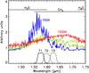 |
Fig. 1 Spectra (Fλ) of model atmospheres of giant planets for different effective temperatures (colored solid lines, BT-Settl models from Allard et al. 2012). Each spectrum is normalized to its value at 1.6 μm and is vertically shifted by a constant. The transmission of the three SDI filters of NaCo (T1, T2, and T3) are shown in black lines with different styles. Theoretical absorption bands of water and methane are also indicated. The vertical scale is linear. |
Based on a complete compilation of young and nearby stars recently identified in young co-moving groups and from systematic spectroscopic surveys, a subsample of stars, mostly AFGK spectral types, was selected according to their declination (δ≲ 25°), age (≲200 Myr), distance (d ≲ 25 pc), and R-band brightness (R ≲ 9.5) to ensure deep detection performances. The age cut-off ensures that the cool companions detected will have masses within the planetary mass regime. Most targets are members of the nearest young stellar associations, including the AB Doradus (AB Dor) and Hercules-Lyra (Her-Lyr) groups (López-Santiago et al. 2006). The distance cut-off ensures that (i) the probed projected separations are >5–10 AU; and (ii) these targets are the most favorable for detecting cool companions, necessary to fully exploit SDI. The targets are brighter than H = 6.5 to ensure good sensitivity with the narrow (Δλ = 0.025 μm, Δλ/λ ~ 1.6%) SDI filters of NaCo, while they are bright enough in the visible to allow good AO efficiency.
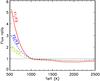 |
Fig. 2 Flux ratio as a function of the effective temperature derived for the NaCo SDI filters (Fig. 1). F1, F2, and F3 refer to the fluxes in the filters at 1.575, 1.600, and 1.625 μm, respectively. The theoretical relations are derived for a given age of 70 Myr, so the surface gravity of the object log (g) is not constant. It increases from 3.75 to 4.75 for the plot range. We also consider the same photometric zeropoint for all the SDI filters. |
The properties of the 16 observed targets are summarized in Table 1 and Fig. 3. The spectral types and the distances are taken from the SIMBAD database2, and the H-band magnitude from the 2MASS catalog (Cutri et al. 2003). The ages are derived from individual sources listed in Table 1. The targets that do not comply with the selection criteria given above are either backup targets or targets for which the age was underestimated at the time of the observing proposal.
Observational and physical properties of the observed targets.
3. Observations and data reduction
3.1. Observing strategy
NaCo offers several high-contrast imaging modes, and the objective of our program was to take advantage of those that are relevant to test the interpretation of the SPHERE data. We combined the four-quadrant phase mask (FQPM, Rouan et al. 2000), the pupil-tracking mode, that allows ADI observations, and the SDI mode, which is based on the concept of the TRIDENT instrument on the Canada-France-Hawaii Telescope (Marois et al. 2003). In this section, we refer to the combination of these techniques as ASDI-4, or as ASDI when the FQPM is not used (for reasons related to the observing conditions, see Sect. 3.2). In the latter case, the images were saturated to compensate for the loss of dynamic at the cost of a higher photon noise in the inner part of the PSF. Phase masks were installed in NaCo as soon as 2003 (Boccaletti et al. 2004) and have produced astrophysical results (Gratadour et al. 2005; Riaud et al. 2006; Boccaletti et al. 2009, 2012).
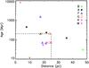 |
Fig. 3 Age-distance diagram of the star sample observed in the NaCo SDI survey. The dashed lines indicate the criteria used for the sample selection (age ≲ 200 Myr and distance ≲ 25 pc). |
Although the star attenuation provided by the FQPM is chromatic, Boccaletti et al. (2004) show that the contrast achieved for a given spectral band is not limited by chromaticity effects induced by the low spectral resolution and/or by small differential aberrations, because the coherent energies measured by the wavefront sensor are modest (≲50% at 2.17 microns). This will also be the case in H band, for which the AO correction is worse. The SDI mode is based on a double Wollaston prism (Lenzen et al. 2004; Close et al. 2005), which produces four subimages on the detector in front of which is set a custom assembly of three narrow-band filters (Fig. 4, left). The central wavelengths of these filters are λ1 = 1.575 μm, λ2 = 1.600 μm, and3λ3a = λ3b = 1.625 μm. The platescale of the SDI camera is ~17 mas/pix. SDI was upgraded in 2007 to provide a larger field of view (8′′ × 8′′, limited by a field mask to avoid contamination between the subimages) and a lower chromatic dispersion of each point spread function (PSF). The differential aberrations between the four images were measured to be lower than 10 nm rms per mode for the first Zernike modes using phase diversity (Lenzen et al. 2004). The combination of the FQPM and SDI modes was commissioned by some of us using AB Dor (H = 4.845) as a test bench (Boccaletti et al. 2008). The seeing conditions estimated by the Differential Image Motion Monitor (DIMM) were good (0.78 ± 0.12′′, λ = 0.5 μm), as was the coherent energy measured by the visible (0.45–1 μm) AO wavefront sensor (52 ± 4%, λ = 2.17 μm). We measured a noise level, expressed as the contrast to the star, of 10-4 at only 0.2′′ after applying SDI and ADI on ten images covering 50° of parallactic rotation (exposure time of 936 s for each image). However, this noise level does not consider the self-subtraction of off-axis objects occurring in SDI. Consequently, it cannot be used to derive mass constraints on detectable companions.
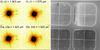 |
Fig. 4 Left: single raw image of a target star provided by the SDI mode of NaCo. The wavelength of the four subimages is from the top right in the anticlockwise direction: 1.575, 1.600, 1.625, and 1.625 μm. The image is thresholded and the scale is logarithmic. Right: flat-field image of the SDI filters (the vertical bars of the filter support are visible in the top half of the image), the double Wollaston prism (which produces the four subimages) and the FQPM (the cross visible in each subimage). The image scale is linear. Both image sizes are 1026 pixels × 1024 pixels, and the field of view of each subimage is 8′′ × 8′′. The cut of the images seen on their left side is due to the position of the field selector on the light beam. Note the inverted tints of both images. |
Log of the observed targets.
Assuming that atmospheric speckles average out over time, both SDI and ADI are intended to attenuate the quasi-static stellar speckles. In ADI, the quasi-static speckles located in pupil planes are kept at a relatively stable position with respect to the detector, while the field of view rotates in a deterministic way. The ability of ADI to suppress speckles directly depends on the stability of the telescope, the AO correction, and the instrument. In SDI, images at different wavelengths are obtained simultaneously, and the quasi-static speckles move radially while an off-axis object (a planet for instance) remains at the same position. The performance of SDI is limited by the differential aberrations and the chromatic dependence of the speckles, which is considered linear in first approximation. If this is true for the geometrical aspect (position and size of the speckles), the wavelength dependence of the phase can be nonlinear due to chromatism (Marois et al. 2006b). The two techniques benefit each other if combined. In this work, they are combined sequentially with SDI first to attenuate the temporal dependence of the speckles and then with ADI to reduce the impact of chromaticity.
3.2. Data acquisition
The data result from three programs carried out in visitor mode in August 2010 (085.C-0257A) and December 2010 (086.C-0164A), and in service mode in October 2011 (088.C-0893A). The observing log is given in Table 2. The observing conditions vary from medium (mean seeing ϵ = 0.7–1′′) to very bad (ϵ> 1.4′′). The durations of the observing sequences are 30–180 min. The amplitude of the parallactic rotation Δθ varies from 10° to 155° according to the observing time and the star’s declination. For the ASDI-4 observations, the single exposure time (DIT) is chosen to fill ~80% of the full well capacity of the detector (15 000 ADU). For the ASDI observations, the star’s image is saturated to a radius about five to seven pixels to increase the dynamic range in the regions of interest. Because the field of view is relatively small, the azimuthal smearing of off-axis point sources remains negligible even for the highest DIT value (30 s). A data set is composed of Nexp datacubes containing DIT × NDIT frames.
A defect in the setting of the pupil-tracking mode leads the star image to drift across the detector4. This is a very unfavorable situation for coronagraphy, especially for high zenithal angles. For this reason, each datacube is limited to a duration of 30–60 s in order to adjust the star image behind the coronagraphic mask online. For HIP 118008 and HD 38678, we did not use the coronagraph because of a large drift and very unstable observing conditions, respectively. For Fomalhaut, the coronagraphic mask was not allowed in service mode at the time of the observation.
At the end of each observing sequence, a few sky frames are acquired around the observed star, essentially for the purpose of subtracting the detector bias (the sky itself being fainter than the bias for the narrow SDI filters5. Before each observing sequence, we record out-of-mask images of the star, with or without a neutral density filter depending on the star magnitude, to determine the PSF and to serve as a photometric calibration.
3.3. Data reduction
The data are reduced with the pipeline described in Boccaletti et al. (2012), which was modified to take the specificities of SDI data into account. This pipeline operates in two steps:
-
1.
step 1: constructing the “reduced” mastercubes for the scienceimages and the PSF;
-
2.
step 2: applicating the differential imaging methods, SDI and/or ADI.
3.3.1. Science and PSF “reduced” mastercubes
An example of a single frame recorded at the detector is shown in Fig. 4 (left). In the first step, all single frames are corrected for bad pixels and flat field. However, when using the FQPM combined to SDI, the flat field (FF) correction requires particular attention. Several optical elements are involved in this configuration (the FQPM, the Wollaston prism, the SDI filters), each being located on different filter wheels. Some of them are close to a focus (the FQPM and the SDI filters), so are very sensitive to dust features. The dust features (Fig. 4, right) generate variations in the pixel transmission as large as 20%. Given the accuracies of the wheel positioning, the relative positions of the optical elements are not the same from one observation to another.
The detector FF is measured on twilights with the H-band filter. Standard calibrations obtained with the internal lamp provide the FF of some combinations of elements (SDI filters, SDI filters + Wollaston prism, SDI filters + Wollaston prism + FQPM). A FF of all the optical elements (SDI filters + Wollaston prism + FQPM) is shown in Fig. 4 (right) for illustration. We can see for each subimage the square-rounded-corner field stop and the trace of the FQPM transitions. We also note the edges of the filter assembly (one edge appears in the upper right subimage). From these calibrations, we extract the FF of each individual element. Then, for most targets, an image of the configuration SDI filters + Wollaston prism (+ FQPM) is recorded at the beginning of the observation. This image cannot be used as a FF because of a poor signal-to-noise ratio (integration time of 2 s instead of 9 s for a regular FF). Instead, it is used as a reference for the realignment of the individual FFs to produce a combined FF. For two stars (HIP 10602 and HIP 18859), the preimaging of the configuration is not recorded. For these cases, in addition to the detector FF, we only correct for the averaged transmission in each subimage. Therefore, the small-scale patterns like dust features on the FQPM are not removed. Finally, the FF is normalized to the median value over the pixels containing signals, hence excluding the field stop and the edges of the filter assembly. The averaged transmission factors in the SDI quadrants are ~0.93, ~0.95, and ~1.07 for the subimages I1, I2, and I3a/I3b respectively. The precision of the FF correction is 10% to 20% for the two stars without the preimaging of the instrumental configuration. It is ~4% for the other targets and set by the centering precision of the regular FF (0.2 pixels).
For the PSF images, several datacubes are recorded each containing several frames. For a datacube, we subtract a mean sky background image of the same duration than the individual images, extract the SDI quadrants, recenter the star image on the central pixel using Gaussian fitting, and average these frames. All datacubes are processed similarly and then averaged, producing a (x,y,λ) PSF mastercube normalized in ADU/s and corrected for the neutral density transmission (1.23% ± 0.05% as reported in Boccaletti et al. 2008; Bonnefoy et al. 2013, we actually use 1/80 in the data reduction).
For the science images, the first important step is to select frames, in particular, to reject open AO loops. The selection is based on the number of pixels νf (f, the index of a frame) in a given subimage (Fig. 4, left) for which the flux is superior to an intensity threshold. This quantifies the width of the star image, a close-loop image having more pixels above this threshold than an open-loop image. After trials, we set this threshold to 60% of the maximum flux measured on a single datacube. Then, we retain the images for which the number of pixels νf is greater than 40% (70%) of the maximum value of νf for coronagraphic (saturated) data. The threshold is higher for saturated images, since the flux can be high even in open-loop images.
Our procedure performs an efficient rejection of the open-loop images. The selected frames are averaged per groups of a few units in order to reduce the frame number in the final mastercube to about a hundred or so (issue related to computing time when applying the differential imaging, Sect. 3.3.2). The binning values ensure that the smearing of off-axis point sources at the edges of the images remains negligible. If the frame bin is not an integer multiple of the number of frames in a datacube after selection, the remaining frames are averaged and accounted for in the mastercube. For the purpose of ADI, a vector of parallactic angles (averaged in a frame bin) is saved. Then, an averaged sky background image is subtracted out frame by frame to the mastercube. We do not apply any linearity correction on the raw frames. However, the nonlinear regions are not taken into account for the image normalization (the PSF are not saturated) or the estimation of the flux rescaling factor for the SDI processing (Sect. 3.3.2). No astrometric calibration is applied, so that the orientation of the True North is known with low accuracy (0.5–1°).
In addition to filter open-loop images during the construction of the mastercube, a second level of selection is applied to the mastercube in order to reject the frames of lower quality (poor AO correction, large seeing, large offset from the coronagraphic mask, etc.). For these data, we base our statistical analysis on the total flux in one subimage, but other criteria are available in our pipeline. The frames departing from the median flux by X times the standard deviation are eliminated from the mastercube. For most stars in our sample, we use X = 2 (5% of images rejected), except for Fomalhaut for which we select X = 3 (1% of images rejected). These values are chosen to reject the worst frames, while reducing the discontinuities in the temporal sequence. Indeed, large temporal discontinuities introduce biases in the ADI construction of the star reference image. In particular, the observing sequence on Fomalhaut suffers from large discontinuities. After selection, the vector of parallactic angles is updated, and the temporal mastercube (x, y, t) is separated to form a four-dimensional (x, y, t, λ) mastercube.
Before the registration of the “reduced” mastercube, the frames for each subimage are recentered using function-fitting. For saturated images, the most robust results are obtained with Moffat function-fitting6 (Moffat 1969), in which the central saturated region is assigned a null weight. For coronagraphic images, centroiding algorithms are not efficient, since the coronagraph alters the intensity and the shape of the star image as a nonlinear function of the pointing. Therefore, we follow the same process as described in Boccaletti et al. (2012), where the fit of a Moffat function is applied on images thresholded at 1% of their maximum. It has the advantage of putting the same weight in all pixels within a given radius to the star (~0.75′′) and to damp the impact of nonlinearities in coronagraphic images.
In Table 2 (three last columns), we provide the frame binning (number of co-added frames), the frame number in the science mastercube, and the total exposure time for all targets. The value of the latter is approximate as long as the number of frames per datacube is not always an integer multiple of the frame bin.
3.3.2. SDI and ADI algorithms
Since SDI is obtained from simultaneous images, it has the capability of reducing the impact of evolving stellar speckles, which usually limit the performance of ADI. Therefore, SDI should be applied in the first stage. The principle of SDI is already described in Racine et al. (1999), Marois et al. (2000), and Biller et al. (2007), but we briefly recall it for the purpose of this paper. Two images of a star (science image Is and reference image Ir) at different wavelengths but spectrally adjacent are aligned, set to the same spatial scale, scaled in intensity to correct for differential filter transmission and stellar flux variations, and finally subtracted. If we assume λr>λs, which corresponds to our data, this implies that the reference image Iris reduced in size by a factor λr/λs. In our pipeline, the intensity scaling factor is derived from the ratio of the total fluxes measured in annuli of inner and outer radii 0.2′′ and 0.5′′ respectively. We did not optimize these values, but we have checked that we are in the intensity linear regime. After the subtraction, the star contribution is strongly attenuated, while the signature of a putative planet is composed of a positive component at the separation of the planet and a negative component closer in separated by 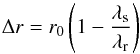 (1)with r0 the planet separation in the science image Is. As Δr increases with r0, the overlapping between the positive and negative components of the planet decreases with the angular separation. The bifurcation point (rb), as defined by Thatte et al. (2007), is the angular separation beyond which the spacing between the positive and negative companion components is greater than the PSF width in the science image λs/D (with D the telescope diameter). Using this definition in Eq. (1) and rearranging the terms for expressing the bifurcation point, we obtain
 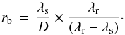 (2)In our data reduction, where four subimages are available, we consider all subtractions. We note the subtraction
  , with
  the reference image rescaled spatially and photometrically. Thus, the subtractions are I13a, I13b, I23a, I23b, and I12 (Fig. 4, left). For the VLT (D = 8.2 m), the bifurcation point is 1.3′′ for the two first subtractions and 2.6′′ for the three last ones. However, this is valid for diffraction-limited images (full width at half maximum FWHM = 40 mas), which is not the case for our data (FWHM = 57–120 mas). This implies that the point-source overlapping will be more significant at a given separation, so the SDI performance will be degraded (Sect. 4.1).
We apply SDI to each couple of frames in the temporal sequence. An output four-dimensional datacube is produced, with the number of subtractions as the fourth dimension. ADI is applied at a second stage. We consider two algorithms, classical ADI (cADI, Marois et al. 2006a) and the Karhunen-Loève Image Processing (KLIP, Soummer et al. 2012). The processed image is smoothed on boxes of 3 × 3 pixels, approximately the PSF FWHM, in order to filter the high-frequency noise. Finally, we derive the contrast levels of the residual noise using the standard deviation of the image residuals on rings with one-pixel width for all separations. Figure 5 shows the median 1σ noise level of the survey with ADI and ASDI, together with the worst and best cases based on the performance reached at 0.5′′. We consider the image I1 for ADI and the subtraction I13b for ASDI. We account for the attenuation of ADI for both methods by injecting seven synthetic planets in the raw data at separations of 0.3, 0.5, 1, 1.5, 2, 3, and 4′′ in two directions separated by 180° to avoid overlapping. The largest parallactic rotation in the survey is 155° (Table 2). Nevertheless, we neglect the SDI attenuation, since it depends on the spectral properties of companions that could have been detected (Sect. 4). This is equivalent to assuming that the companion contains methane and does not emit flux in the I3b image. We note that the worse the observation quality the smaller the difference between the ADI and ASDI noise levels. For the median curves, we see that ASDI improves by a factor ~2–3.5 the noise level at separations closer than 1.5′′, where speckle noise dominates background noise. Nonetheless, ASDI slightly degrades the detection performance for larger separations, where background noise is the dominant source of noise. In particular, ASDI potentially offers a gain in angular resolution of 0.2–0.4′′ to search for faint companions of a given contrast at separations of 0.3–1′′. We explain in Sect. 4 that while the residual noise can be used to determine the sensitivity limits in planet mass in ADI imaging, this method is no longer valid in SDI or ASDI imaging.
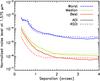 |
Fig. 5 Residual noise in the I1 image expressed in contrast with respect to the star after ADI alone (solid lines) and after ASDI (dashed lines). We consider for ASDI the subtraction I13b. We represent the median, best, and worst curves in the survey (colored curves, see text). We account for self-subtraction from ADI for all curves using synthetic planets, but not from SDI for the ASDI curves (see text). |
3.4. Photometric errors
We summarize here the different sources of photometric errors in the data reduction and analysis that affect the noise levels shown in Fig. 5:
-
The correction of the neutral density transmission. Thistransmission is measured with a precision of 4%.
-
The correction of the pupil Lyot stop associated with the FQPM. This diaphragm is undersized by 10% in diameter with respect to the full aperture, so the geometrical throughput is 0.808. However, Boccaletti et al. (2008) report an uncertainty of 4% on this value, probably due to optical misalignments of the entrance pupil of NaCo. For the coronagraphic observations, we kept the Lyot stop for the measurement of the PSF to minimize this error source, except when the neutral density is used.
-
The photometric stability due to variations in the AO correction and, for the coronagraphic observations, variations in the FQPM centering. The PSF is measured once at the beginning of the observing sequence. Consequently, we cannot estimate the temporal variability of the PSF. We use the science images and measure the variability of total intensity in an annulus between 0.2′′ and 0.5′′ (region in the linear regime) for all targets. The median value at 1σ is 12% (range 6–17%).
4. SDI data analysis
In this section, we first introduce the theoretical formalism of the flux measurement in SDI-processed images (Sect. 4.1) and argue that, contrary to single-band imaging surveys, the residual noise cannot be converted into mass limits through evolutionary models, because it represents a differential flux. This differential flux can be accounted for by several planet masses, resulting in degeneracies for the mass limits (Sect. 4.2). The degeneracies can be removed with the use of single-band detection constraints. Finally, we describe the method used for the analysis of this survey, which is based on synthetic planets and model fluxes to directly determine the mass limits (Sect. 4.3).
4.1. SDI signature
In the general context of high-contrast imaging with a single spectral filter, the detection limits are measured on contrast maps. In most cases, the azimuthal standard deviation is used to derive one-dimensional contrast curves. These curves are then corrected from various attenuations (ADI and/or coronagraph) and converted into mass limits according to a given evolutionary model. The problem of SDI is different because we measure a differential intensity. The sign and modulus of this residual intensity at the location of an object depend on its spectral shape (at the first order determined from its temperature), as shown in Fig. 1, and on its separation in the image. It can be expressed as follows (no coronagraph and no ADI): 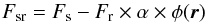 (3)with Fs and Fr the object fluxes in the science and reference images, α the intensity rescaling factor, φ(r) the attenuation due to the spatial rescaling, and r = (r,θ). The dependency of φ(r) on θ is related to the PSF structure (see below), where φ(r) = 1 means that the planetary companion is close to the star so that the positive and negative components of its SDI signature mostly overlap and cancel each other out. This is the worst case for SDI in terms of performance. On the contrary, φ(r) ≃ 0 means that the processing does not attenuate the planet intensity, i.e. Fsr ≃ Fs, which is the optimal case. The factor φ(r) can be determined for each radial separation and azimuthal direction using measured or modeled PSF in each couple of filters. Knowing the characteristics of φ(r) is important for data reduction and interpretation of the detection limits (Sect. 5). We briefly discuss here key points relevant to the survey analysis, while a companion paper will address the SDI biases in detail (Rameau et al. in prep.).
First, the SDI geometrical attenuation φ(r) depends on the wavelengths of the images used for the SDI subtraction. For a given separation in the image, the larger the spacing between the wavelengths, the smaller φ(r) (Eq. (1)). In particular, we saw that the bifurcation point is smaller for the I13b subtraction than for the I23a subtraction (Sect. 3.3.2). We also note that the flux ratio F1/F3 is greater than the flux ratio F2/F3 for cool giant planets (Fig. 2). As a result, the self-subtraction will be less for the I13b subtraction (Eq. (3)). Thus, we consider only this subtraction for the data analysis.
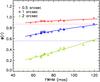 |
Fig. 6 Azimuthal mean of the geometrical SDI attenuation factor φ(r) derived for all the observed stars and the I13b subtraction at separations of 0.5, 1, and 2 arcsec (colors) as a function of the FWHM (see text). The dotted lines indicate the values for a diffraction-limited PSF. The solid lines are power-law fitting laws. |
For a given wavelength couple (λs, λr), the SDI geometrical attenuation φ(r) is a function of the position in the image field, both radially and azimuthally. These dependencies are intimately related to the PSF properties. We use real data to derive φ(r) to take PSF structures that cannot be modeled into account. We determine φ(r) from the flux ratios of a PSF measured in the I1 and I13b images. Both fluxes are summed in apertures of 3 × 3 pixels centered on the PSF location in the I1 image. Figure 6 represents the azimuthal mean of the SDI geometrical attenuation (noted φ(r) in the remainder of this paragraph) measured at three separations for all the stars in the survey as a function of the FWHM. The FWHM is estimated using the mean value from several methods (Gaussian fitting, radial profile). The typical standard deviations are 0.3–0.4 pixels, but can be as much as ~1 pixel for elongated PSF. The values of φ(r) for a diffraction-limited PSF are also indicated as dotted lines. For a given star (same FWHM), we observe that φ(r) decreases with the separation. The measured values are greater than the theoretical values, since the images are not in the diffraction-limited regime (Sect. 3.3.2). We also note that the larger the separation, the greater the discrepancy between the measured and theoretical values. For a given separation, we observe that the range of the measured φ(r) increases. At small separations, φ(r) is close to 1 (Eq. (1)), and the self-subtraction is large and depends little on the PSF properties. As the separation increases, φ(r) diminishes, and the dependency of the self-subtraction on the PSF quality is stronger. We determine that the best fitting law for this behavior is a power law. We note that the fitting laws agree with the diffraction-limited values of φ(r) at the theoretical value of the FWHM for the smallest separations. The discrepancy seen for 2′′ could be accounted for by a different behavior of φ(r) with this parameter in (nearly) diffraction-limited regimes, as expected for SPHERE and GPI. We tested possible correlations of φ(r) with other observational factors, the Strehl ratio, coherent energy, correlation time of the turbulence, and seeing (results not shown, see the detail of the estimation methods in Appendix A.1). We find correlations with the Strehl ratio alone. We conclude that the PSF FWHM is an important parameter for interpreting the SDI performance at separations beyond 0.5′′. This is also true for ASDI (see Sect. 5).
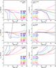 |
Fig. 7 Differential flux F13b of a planet predicted by the evolutionary model BT-Settl (Allard et al. 2012) as a function of mass for all targets and three separations (rows). The stars are sorted by age, <100 Myr (left column) and ≥100 Myr (right column). The top right part of the right panels shows the curve for HIP 114046, which is a very old star (8 Gyr, Table 1). |
Finally, the SDI geometrical attenuation φ(r) (so the SDI performance) is a function of the direction in the field of view θ, owing to PSF asymmetries. For a few observations, the PSF is elongated because of an astigmatism not corrected by the active optics system of the telescope. This must be accounted for when deriving SDI (so ASDI) sensitivity limits. The method that we use for assessing the detection limits of the survey accounts for this point (Sect. 4.3).
4.2. Degeneracy of the differential flux with the planet mass
When a low-mass object is detected in an SDI-processed image and providing φ(r) is calibrated, one can test the individual intensities Fs and Frfor all planet masses in an evolutionary model that reproduce the measured differential flux Fsr (Eq. (3)). Although no practical case has been published in the literature yet, we expect that several values of Fs and Frcan match the observations, which results in degeneracies for the mass estimation. The number and the values of the mass solutions depend on φ(r), so on the position in the image.
Figure 7 shows the differential flux F13b predicted by the BT-Settl models (Allard et al. 2012) as a function of mass for three values of φ(r). To obtain these curves, we derive the fluxes in Eq. (3) from the model absolute magnitudes and assume φ(r) = φ(r) and α = 1; i.e., the flux measured in the reference image F3bis corrected for the differences in flux and filter transmission. For the conversion of absolute magnitudes into fluxes, we consider the star distance, the star magnitude in H band, and the maximum of the measured PSF in the corresponding filters for the photometric zeropoints. Using the H-band magnitude for the magnitude in the SDI filters is equivalent to assuming that the stellar spectrum in this spectral region does not exhibit features (Rameau et al., in prep.). The curves shown in Fig. 7 are specific to the choice of stellar parameters considered in this paper. Using different parameters (in particular the star age) will produce different curves. We chose to express the differential flux F13b in ADU/s in order to represent the data for all stars. We must take the actual integration time of the observation into account to test the ability to distinguish potential degeneracies of F13b with the mass.
For separations closer than 0.2′′ (Fig. 7 top row), the differential flux F13b is negative for masses greater than 3–25 MJ according to the stellar age, while it is positive for lower masses. This is consistent with Fig. 1. For temperatures higher than ~1000 K (≳4 MJ at 10 Myr and ≳10 MJ at 100 Myr), there is no methane absorption at 1.625 μm, while methane absorbs the flux for lower temperatures. In some cases, we find that F13b is accounted for by two or three values of the companion mass. The number and the values of the degeneracies depend on the stellar properties (and on the position in the image, see below). The degeneracies correspond to low values of F13b, typically inferior to 0.5 ADU/s for stars younger than 200 Myr. Consequently, long integration times will be required to reach the photometric accuracy needed to detect the degeneracies.
For separations around 1′′ (Fig. 7 middle row), we note three regimes for F13b. It is positive for low masses, then negative for intermediate masses, and finally positive for massive objects. The reason for the existence of this last regime is that after the flux ratio F1/F3b diminishes below 1 when there is no methane absorption anymore, it increases toward one for temperatures higher than ~2100 K (Fig. 2). We retrieve degeneracies of F13b with the mass for some cases, but different due to a different φ(r) value. We also find new degeneracies for negative F13b.
For separations of ~4′′ (Fig. 7 bottom row), F13b is positive regardless of the mass because F13b = F1, and increases with the mass. For a few targets (HIP 10602, and the stars younger than Fomalhaut in the right panel), degeneracies appear for ~10–20 MJ. These degeneracies are inherent to the evolutionary model.
One possible solution for removing the mass degeneracies is to measure the flux of an object in a single filter if it is detected, after data processing with ADI, for instance. We show in the next section that in the case where no object is detected, the mass degeneracies inherent to SDI also affect the assessment of the detection limits, implying the need to compare the constraints of ASDI to those of single-band differential imaging.
4.3. Detection limit
When no object is detected in an SDI-processed image, the situation is more complex. The residual image exhibits positive and negative intensities with strong pixel-to-pixel variations resulting from the image subtraction. As long as we should expect a low-mass object to also have either positive or negative flux, it becomes difficult to disentangle the noise from a signal. Thus, the method used for single-band surveys (ADI, coronagraphy), which consists of building a contrast map from the standard deviation and converting it into mass, is no longer valid. A variation of this method will be analyzed thoroughly in a companion paper (Rameau et al., in prep.). Such a method requires good determination of both ADI and SDI attenuations (φ(r)). Here, we apply a more straightforward and robust technique based on injecting synthetic planets into the data set at the cost of a longer computing time and sparsity in the detection map. The use of synthetic planets is common in high-contrast imaging. For this work, we use the measured PSF for each data set for the whole corresponding temporal sequence. Thus, we assume that the PSF is the same in the science and the PSF images. This hypothesis strongly depends on the AO-loop and photometric stabilities, and we should expect variations from one data set to another.
We consider a given evolutionary model where the absolute magnitudes of low-mass objects are tabulated for different ages and masses in the SDI filters. Assuming the age and the distance for a given star, we obtain the expected flux for a given planet mass. Twelve synthetic planets are simultaneously injected in empty datacubes at the positions 0.3, 0.5, 0.7, 0.9, 1.1, 1.4, 1.7, 2, 2.5, 3, 3.5, and 4′′. They are also introduced at several position angles. For each case, we take care that the planets do not overlap, because of the SDI spatial rescaling and the ADI field rotation. The resulting datacube is processed with ASDI and ADI as described in Sect. 3.3.2. We measure the residual intensities of the planets using aperture photometry (Sect. 4.1). For each separation, we azimuthally average the fluxes.
The noise is measured in the data processed without the synthetic planets (Sect. 3.3.2) and scaled to the same aperture size assuming white noise. The process is repeated for each model mass in order to obtain a three-dimensional array of signal-to-noise ratio versus mass and separation. For each separation, we interpolate the signal-to-noise ratio versus mass relation to determine the mass and effective temperature achieved at 5σ. We checked that the detection limits (Sect. 5) are consistent with the reduced datacubes containing the data and the synthetic planets. Figure 8 shows examples of curves of the signal-to-noise ratio as a function of planet mass for HIP 118008 and several separations for ADI and ASDI. For a given mass, it increases with the separation, because the noise level diminishes. For a given separation, it increases monotonously with the mass for ADI but not for ASDI. For the latter case and a signal-to-noise ratio of 5, a degeneracy is observed around 0.6′′ (6, 8.5, and 10.5 MJ). However, it is removed when comparing it to the ADI constraint, which is deeper (objects ≥5.5 MJ excluded). We encountered several degeneracies in the data analysis, but we excluded all of them using ADI.
The errors on the signal-to-noise ratios (and the sensitivity limits, Sects. 5 and 6) are induced by the errors on the noise level (Fig. 5) and on the measured flux of the synthetic planets. We summarize the contributors to the latter below:
-
the photometric stability of the PSF (~12%,Sect. 3.4);
-
the stability of the PSF FWHM. We evaluate it using the coherent energy estimated by the wavefront sensor: the median variability of the coherent energy is 14% (range 6–30%). This translates into a FWHM variability of 12% (median value, range 8–20%);
-
the uncertainties on the star magnitude and distance (median combined error for the flux 9%). We assume that the star magnitude is the same in the H band and in the SDI filters;
-
the photometric extraction. We derive the fluxes in apertures of 3 × 3 pixels (width 52 mas), while the measured FWHM are 57–120 mas (Fig. 6).
We evaluate the impact on the signal-to-noise ratio for an error budget of 20% on the PSF photometry to ~30%. This translates into errors on the planet mass of 5–1 MJ (~200–100 K) for a range of 50–7 MJ (Sects. 5 and 6).
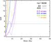 |
Fig. 8 Signal-to-noise ratio of synthetic planets measured in the images of HIP 118008 after ADI (solid lines) and ASDI (dashed lines) as a function of mass for several separations. The cut-off at low masses is due to the evolutionary model BT-Settl (see text). The horizontal dotted black line indicates the signal-to-noise ratio used to derive the mass sensitivity limits (see text). |
For this work, we use the 2012 release of the evolutionary model BT-Settl (Allard et al. 2012). This model simulates the emergent spectrum from the atmospheres of giant planets, brown dwarfs, and very low-mass stars for given values of effective temperature, surface gravity, and metallicity7. It then uses the evolutionary tracks of the COND model (Baraffe et al. 2003) to associate the spectrum parameters to the age and the mass of the object. With respect to previously published models (Burrows et al. 1997; Chabrier et al. 2000; Baraffe et al. 2003), BT-Settl accounts for the cloud opacity. We select a subgrid in the model, spanning effective temperatures from ~500 to 4000 K. The low cut-off in effective temperature implies that the minimum planet mass available at a given age increases with the latter (from 1 MJ at 10 Myr to 5 MJ at 200 Myr). Although BT-Settl models atmospheres with effective temperatures well below the condensation temperature of methane, we reach the model boundary for half of the targets (Sect. 5). For these cases, we cut the sensitivity limits at this value. The limitation of the BT-Settl predictions to temperatures above ~500 K is due to poor knowledge of infrared molecular lines of methane and ammonia at lower temperatures (Allard et al. 2012). Modeling colder atmospheres could be necessary for the data analysis of SPHERE and GPI, since we expect higher contrast performance than for NaCo. We discuss the use of the BT-Settl evolutionary model and the dependence of the results on this model in Sect. 6.4.
We summarize the key conclusions of the whole section.
-
1.
The residual noise measured in SDI-processed images cannotbe converted into mass limits in the same way as used forsingle-band imaging surveys. This led us to develop a methodbased on synthetic planets and flux predictions to directlyestimate the mass limits.
-
2.
The assessment of the detection limits, as well as the photometric characterization based on SDI data, face degeneracies in the planet properties. This implies that interpreting SDI data requires an analysis that couples ASDI and single-band imaging.
-
3.
The spectral overlapping of an off-axis source φ(r) is strongly affected by the PSF FWHM for large separations (>0.5′′). We thus expect that the PSF FWHM is a parameter to consider when studying the ASDI detection limits.
5. Results
The data analysis does not yield any detections. We discuss below the mass sensitivity limits (Sect. 5.1). Then, we analyze the limits in effective temperatures (Sect. 5.2). We conclude with a detailed study of the ASDI performance (Sect. 5.3).
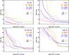 |
Fig. 9 Detection limits in mass of the survey according to the BT-Settl evolutionary model (Allard et al. 2012) after ADI applied to the I1 image (solid curves) and after ASDI performed for the I13b subtraction (dashed curves). The stars are sorted by increasing age from left to right and from top to bottom. The curves are cut when the minimum mass covered by the evolutionary model is reached (see text). |
5.1. Mass detection limits
We represent the mass detection limits derived for ADI as a function of the angular separation in Fig. 9. The stars are sorted by age categories in the panels. As expected, the lowest mass achievable increases with the star age, from 1–4 MJ for stars younger than 70 Myr (top left), to 10–31 MJ for stars older than 200 Myr (bottom right). As mentioned in Sect. 4.3, the sensitivity limits are cut when the lower mass available in the evolutionary model is reached. Nevertheless, the performance at small separations (≲1′′) clearly depends on other parameters, as we can see in the top righthand panel, which shows stars with the same age8. Good observing conditions (HIP 18859), large parallactic rotations (HIP 118008), and good image dynamic (indicated by the star magnitude and the total exposure time, Tables 1 and 2) ultimately account for the performance. The median sensitivity limits are 47, 19, and 9 MJat 0.3, 0.6, and 1′′.
The ASDI mass limits are shown in Fig. 9. We give some broad tendencies of the ASDI performance based on our data below as well as in Sects. 5.2 and 5.3. They may not be extrapolated to other published SDI data. We do not see any correlation of the gain provided by ASDI with the star age. There is no particular separation range for which the processing improves or degrades the detection limits. The mass gains can be as large as 10% to 35%. Beyond 1.5′′, ASDI degrades the sensitivity since background noise dominates. The exception is Fomalhaut, because of a higher image dynamic (Table 2). For HIP 102409, HIP 30314, and HIP 106231, ASDI gives worse performance with respect to ADI for all separations. The combined ADI-ASDI median limits are 37, 19, and 9 MJat 0.3, 0.6, and 1′′.
5.2. Effective temperatures
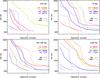 |
Fig. 10 Same as Fig. 9 but for the effective temperature. Note the different vertical scale with respect to Fig. 9. |
A critical parameter that affects the self-subtraction of point sources in ASDI is the flux ratio F1/F3b (Fig. 2). The value of F1/F3b depends strongly on the effective temperature. It is high for values below ~1000 K, close to 1 for the range 1000–1500 K, and it decreases for values between 1500 K and 2100 K. Therefore, we expect a bad performance for ASDI if the raw noise level (before differential imaging) is not sensitive to objects colder than 1000 K, especially in the range 1000–1500 K. We show the sensitivity limits for both ADI and ASDI in Fig. 10. We clearly see the degradation in sensitivity of ASDI with respect to ADI as breaks in the curves at separations of 0.3–1.4′′. Considering all the ADI curves, we reach median temperatures of 1510–784 K at 0.5–1′′. When combining ADI and ASDI, we reach median values of 1507–696 K in the same separation range. We note that the upper limit of the range is nearly the same without or with including ASDI, because it does not usually improve the sensitivity below ~0.5′′.
5.3. Analysis of the ASDI performance
The purposes of this section are to determine, for our data, the condition(s) for which ASDI improves or degrades the sensitivity with respect to ADI and to understand the behaviors seen in Figs. 9 and 10. The detection limits are determined by comparing the residual intensity of synthetic planets to the residual quasi static speckles (Sect. 4.3). A planet flux is attenuated by ASDI by a quantity determined in part by its spectral properties (presence/absence of methane absorption bands, Fig. 1) and φ(r), which quantifies the geometric self-subtraction and diminishes with the separation (Sect. 4.1). The quasi static speckles are partially calibrated by ASDI at short separations (≲1–2′′), except for HIP 106231 (Fig. 5). ASDI improves (respectively degrades) the sensitivity if the speckle attenuation is larger (resp. smaller) than the planet self-subtraction.
We first determine the ASDI speckle attenuation as a function of the ASDI self-subtraction of point sources for three angular separations in Fig. 11. The speckle attenuation gains are derived as the ratios of the ADI and ASDI noise levels (Fig. 5). The self-subtraction factors are measured from the ratios of the fluxes of synthetic planets measured before and after ASDI (Sect. 4.3), thus including both effects of φ(r) and of the planet spectrum. For information purposes, the points in Fig. 11 are indicated with different symbols, according to the mass gain (Fig. 9, but the curves are not cut to the minimum model mass). While this distinction is consistent with the ratio speckle attenuation/self-subtraction for the two largest separations, it is not always the case for 0.5′′. At this separation, the steepness of the detection limits (Fig. 9) and/or the azimuthal structure of the residual speckles may bias the determination of the mass at 5σ. As expected, we observe that both the speckle attenuation and the point-source self-subtraction diminish with the separation. We see in particular that ASDI affects the sensitivity limits up to a separation of ~2.5′′ (Fig. 9).
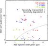 |
Fig. 11 ASDI self-subtraction of point sources as a function of the ASDI speckle attenuation for three angular separations (colors). The points are indicated with different symbols according to the ASDI performance in Fig. 9. The dotted line indicates where the ASDI speckle attenuation equals the ASDI self-subtraction. For the sake of clarity, we do not include the point pertaining to HIP 106231 measured at 0.5′′ (speckle attenuation = 0.9, self-subtraction = 100). |
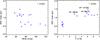 |
Fig. 12 ASDI mass gain as a function of the PSF FWHM (left) and the SDI flux ratio of the companion (right) for an angular separation of 1′′. The labels refer to the points with the best mass gains. |
Another tendency as the separation increases is that the number of stars for which ASDI improves the sensitivity increases (5, 9, and 12 at 0.5′′, 1′′, and 1.5′′, respectively). For a given separation closer than ~1′′, the companion self-subtractions can reach higher values than the speckle attenuations (up to ~10 against ~4), implying that this is the parameter that ultimately drives the ASDI performance. We confirm this point below. We briefly discuss the sources of errors on the quantities represented in the plots described in this section. There is no error bar on the speckle attenuation because normalization errors will affect the images I1 and I3b in the same way and differential errors will not affect the SDI subtraction because the I3b image is rescaled relatively to the I1 image. The ASDI self-subtraction is affected by the PSF errors. The median error is 1. The error on the FWHM due to the estimation methods is 5–7 mas (17 mas for elongated PSF, Sect. 4.1). The error on F1/F3b is induced by the error on the planet mass and is ~0.5 typically. Finally, the error on the ASDI mass gain stems from the errors on the sensitivity limits, and its median value is <0.1.
We conducted a correlation study of the ASDI speckle attenuation and the ASDI self-subtraction in Appendix A. We summarize the results. The ASDI speckle attenuation decreases with the PSF FWHM and the raw noise level (without differential imaging). As for the ASDI self-subtraction, we show that it is mainly correlated to the flux ratio F1/F3b and φ(r), but it also depends on the PSF FWHM for high values at large angular separations.
Finally, we analyze possible tendencies of the ASDI mass sensitivity gain with the FWHM and F1/F3b in Fig. 12 for a separation of 1′′. We computed the mass gains as the ratio of the ASDI and ADI limits (Fig. 9), but without thresholding the curves to the minimum model mass. The mass gains range from 0.5 to 1.5. They no longer exhibit correlations with the FWHM, while they do with F1/F3b. The mass gains are smaller than 1 for F1/F3b ≲ 2 (Teff ≳ 800 K) and greater than 1 above. ASDI provides an improvement in the sensitivity for nine stars, for which we derived the lowest point-source self-subtractions (Appendix A.2). The point-source self-subtraction is thus the critical parameter that determines the performance of ASDI, at least at first order. This confirms the conclusion deduced from Fig. 11. We note that for the mass gains greater than 1, the values are quite constant (~1.1–1.2) with F1/F3b. Nevertheless, three points stand out and present the best mass gains (≥1.2). The corresponding stars exhibit some of the best speckle attenuations (Fig. 11, blue points above ~2.7) and have rather good PSF (FWHM ≲ 67 mas) and/or low raw noise level (≲4.6 × 10⁻⁵). Age also affects the mass gains. HIP 114046 presents the best speckle attenuation (blue point at 3.6), but the smallest mass gain. As for the data points with mass gains below 1, we see an important vertical dispersion. This feature is accounted for by differences in speckle attenuation, the stars with smaller mass gains also having smaller speckle attenuations. The latter are related to the poorer quality of the PSF and of the raw noise level (Appendix A.1).
To summarize the conclusions of this study:
-
1.
the planet flux ratio F1/F3b determines whether ASDI improves ordegrades the sensitivity at first order for separations closerthan ~1′′;
-
2.
when F1/F3b is favorable, good PSF and noise properties improve the mass gain further.
6. Discussion
We first focus on the results for two targets of particular interest (Sect. 6.1). Then, we analyze the broad characteristics of the detection limits. Since the observed sample is quite modest and inhomogeneous, we do not intend to carry out a study of the giant planet frequency, as for published large imaging surveys (e.g., Lafrenière et al. 2007; Chauvin et al. 2010; Vigan et al. 2012; Rameau et al. 2013a; Wahhaj et al. 2013a; Nielsen et al. 2013; Biller et al. 2013). We summarize the properties of the limits in mass (Sect. 6.2) and in effective temperature (Sect. 6.3). Then, we discuss the validity of our hypotheses and the dependency of the results on them (Sect. 6.4). Finally, we discuss some implications of this work for the data analysis and interpretation of the upcoming imaging instrument SPHERE (Sect. 6.5).
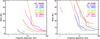 |
Fig. 13 Detection limits in mass using BT-Settl (Allard et al. 2012) and combining several differential imaging methods (see text) as a function of the projected separation. The left panel represents the results for the stars younger than 100 Myr and the right panel those for older targets. The curves are cut according to the maximum projected separation accessible in the SDI field (see text). |
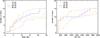 |
Fig. 14 Histograms of the mass (left) and effective temperature (right) detectable at 5σ (Fig. 13) for several physical separations. The maximum number of stars is 16 for 10 AU and 15 beyond (see text). |
6.1. Results for individual stars
6.1.1. Fomalhaut
Fomalhaut is known to harbor a complex system, composed in particular of an outer debris disk with a sharp inner edge at 133 AU resolved by Kalas et al. (2005) and a planetary-mass object closer-in on a highly eccentric orbit (Kalas et al. 2008, 2013). Because the SDI field is limited to 4′′, our images probe the inner part (≲30 AU) of the system. Several teams have observed these regions in order to set constraints on the mass of putative planetary companions. A radial velocity study excludes companions with masses higher than 6 MJ for separations below 2 AU (Lagrange et al. 2013). The analysis of VLT images at 4.05 μm does not yield the detection of objects more massive than 30 and 11 MJ at ~2 and 8 AU (COND model, Baraffe et al. 2003), respectively (Kenworthy et al. 2013). Imaging at 4.7 μm constrains the mass of putative companions below 4 MJ (2.6 MJ) at 9 AU (30 AU) (Kenworthy et al. 2009, COND model). The imaging sensitivity limits are derived assuming the star age from Mamajek (2012). Our narrow-band observations probe the same separation range as in Kenworthy et al. (2009), but with a lower sensitivity of 9–12 MJ based on the same age estimate (Fig. 13, right).
6.1.2. HIP 102409/AU Mic
AU Mic is surrounded by an edge-on debris disk discovered by Kalas et al. (2004). The disk has a parallactic angle of 127° and extends to projected separations of 290.7 AU9. Our SDI images are sensitive to regions closer than ~40 AU. Based on HST and/or ground-based observations and an age estimate of 12 Myr10, several studies set constraints on the mass of planetary companions. According to the predictions of Burrows et al. (1997), HST images presented in Fitzgerald et al. (2007) do not reveal companions of >3 MJ and >1 MJ embedded in the disk at separations larger than 10 AU and 30 AU, respectively. Based on the COND model (Baraffe et al. 2003), VLT/NaCo imaging by Delorme et al. (2012a) excludes giant planets more massive than 0.6 MJ beyond 20 AU, while the analysis of Gemini/NICI data discussed in Wahhaj et al. (2013a) rejects objects of >5 MJ and >2 MJ at separations >3.6 AU and >10 AU, respectively. Although the SDI mode of NaCo is not designed for the observation of extended sources, we detect in the SDI images collapsed in wavelength (I1 + I2 + I3b) and processed with KLIP for several input parameters (Soummer et al. 2012, and Sect. 6.2) the AU Mic debris disk with a poor signal-to-noise ratio per resolution element (method described in Boccaletti et al. 2012) of ≥3 for separations of ~1.5–3.7′′ for the southeast part and ~2.1–3.5′′ for the northwest part. As for the search for planetary companions, our detection limits extend to projected separations down to ~3 AU (>7 MJ) and exclude Jupiter-mass companions beyond 6 AU (Fig. 13, left) according to the BT-Settl model (Allard et al. 2012). These detection limits are azimuthally averaged on the whole field of view. The limits measured along the disk midplane are not significantly different, because the signal-to-noise ratio measured on the disk is weak.
6.2. Characteristics of the mass limits
Figure 13 shows the ultimate mass limits combining several algorithms as a function of the projected separation. We considered cADI and KLIP (Soummer et al. 2012) applied to the I1 image, cASDI and the combination of KLIP and SDI on the I13b subtraction, as well as cADI on the sum of the images I1, I2, and I3b (Fig. 4, left). For each separation, we selected the best limit between the algorithms. We applied KLIP to improve the sensitivity at close-in separations (<0.5′′). The number of modes truncated for constructing the reference images of the stellar speckles is a free parameter of KLIP (Soummer et al. 2012). After some trials, we set the number of modes to one for all stars, except for HIP 98470, HD 38678, and Fomalhaut, for which we chose to retain two, three, and five modes, respectively. To estimate the flux of the synthetic planets after the processing, we first used KLIP on the datacubes containing the data and the planets to derive the principal components for a given number of modes. Then we performed KLIP with these components on the datacubes containing only the planets. We cut the curves at the minimum model mass. We note that certain curves are limited in projected separations due to the size of the SDI field (~4′′ in radius). This especially concerns two stars, HIP 114046 (~13 AU, but the mass cut-off is reached before) and Fomalhaut (~30 AU).
We represent the histogram of the detectable masses for several projected separations in the left-hand panel of Fig. 14. The prime objective of our survey was to search for giant planets at separations as close as ~5–10 AU. Considering an upper mass limit of 13 MJ (Burrows et al. 1997), we observe that eight targets (55% of the sample) satisfy this objective (Fig. 13). We did not take HIP 114046 and HD 10647 into account because of the cut-offs. The limit of 13 MJ is achieved for all targets beyond ~30 AU. The lowest mass achieved is 1 MJ beyond 6 AU around HIP 102409. This star combines several favorable properties, a young age, a late spectral type, and a close distance (Table 1), although the observing conditions are not optimal (Table 2).
6.3. Effective temperature vs. projected separation
The histogram of the temperatures as a function of the physical separation is shown in the right-hand panel of Fig. 14. As for the detectable masses, we cut the detection limits (Fig. 10). The survey is sensitive to companions as cool as 1000 K around 65% of the targets for projected separations larger than 10 AU. The optimal regime for ASDI (Teff ≲ 800 K, Fig. 2 and Sect. 5.3) is accessible for two-thirds of the sample at separations beyond ~20 AU.
6.4. Dependency of the results on the hypotheses
We focus here on the relevance of the hypotheses used for this work and their influence on the results presented in Sect. 5. We recall that the objective of this paper is not to address the unknowns inherent to the considered models, but to outline the difficulties for deriving mass limits from SDI images regardless of the models. We decided to pick one of the available models, so the mass limit presented here should not be considered as absolute values. We based the study on BT-Settl (Allard et al. 2012) because the model temperature range spans values below the methane CH4 condensation temperature, suitable for the search for cool giant planets. This model has the strong point of modeling non-equilibrium chemistry, which might be a key ingredient for understanding the spectral properties of cool young giant planets (Barman et al. 2011a,b). However, it also has caveats, in particular, it is unable to correctly reproduce the transition between M and L dwarfs (Bonnefoy et al. 2014; Manjavacas et al. 2013), and it lacks of opacity in the CH4 band at ~1.6 μm (King et al. 2010; Vigan et al. 2012). We note that the second point is a problem for all current models of planet spectra, because of the incompleteness of the molecular line lists (Allard et al. 2012).
The hypothesis used for the relation between the SDI flux ratio F1/F3b and the effective temperature of substellar companions is critical. Indeed, we showed that F1/F3b is the parameter that determines the ASDI performance at close-in separations to first order (Sect. 5.3). We considered the BT-Settl relation (Fig. 2), which could be pessimistic due to the lack of CH4 absorption at ~1.6 μm. Another possibility is to model the relation on the spectra of observed cool brown dwarfs, as described in Wahhaj et al. (2013b) in the context of the data interpretation of the NICI Campaign. For Teff ~ 750 K, they find F1/F3b ~ 8 based on the spectrum of 2MASS J04151954-093506 (Knapp et al. 2004; Burgasser et al. 2006). BT-Settl gives a value of ~2.111 for the same temperature (Fig. 2). Because φ(r) is larger for NaCo than for NICI (rb ~ 1.3′′ vs. ~0.9′′, Eq. (2)), this results in larger ASDI self-subtractions and worse sensitivity when reaching this temperature at close-in (≲1′′) separations for the NaCo data (Fig. 10). Nevertheless, and as noticed in Nielsen et al. (2013) and Biller et al. (2013), we note that strong CH4 absorptions are measured in the atmospheres of brown dwarfs at temperatures for which we detect little absorptions in those of cool young giant planets (Barman et al. 2011b; Konopacky et al. 2013; Oppenheimer et al. 2013). The only known young giant planet with measured strong CH4 absorption to date is GJ 504 b (Kuzuhara et al. 2013; Janson et al. 2013, Teff ~ 510 K). Using the photometry reported in Janson et al. (2013), we derive F1/F3b > 2.6 (the object is not detected in the CH4 band), whereas BT-Settl predicts F1/F3b ≳ 512 (Fig. 2). We also compare the predictions to other cool (Teff ≲ 1000 K) and young (or proposed as young) objects, HR 8799 b (Barman et al. 2011a) and three T dwarfs (HN Peg B, ROSS 458 C, CFBDSIR2149-0403, Luhman et al. 2007; Burningham et al. 2011; Delorme et al. 2012b). We find close agreement (factors ≲1.2) for the objects with Teff ≳ 1000 K. However, the two cool (Teff ~ 700 K) T dwarfs ROSS 458 C and CFBDSIR2149-0403 show stronger absorptions than predicted by BT-Settl (factors ~2.4). We estimate the maximum values for the differences in magnitude and mass between the BT-Settl predictions and the observed cool brown dwarfs. This corresponds to close-in separations (≲0.5′′), where φ(r) ~ 1 (Fig. 6). We find ~0.85, ~0.5, and ~0.45 mag for the spectral types T4, T6, and T8, respectively (Teff ~1000–700 K). Using BT-Settl isochrones, these values translate into underestimations for our ASDI detection limits with respect to the use of observed brown dwarfs of ~1–2 MJ for an age of 70–200 Myr(Figs. 9 and 10). For larger separations, these estimates are decreased because φ(r) is smaller.
To conclude this analysis, we outline that the interpretation of SDI data is model-dependent, as it is when assessing sensitivity limits in terms of planet parameters. In particular, the ASDI self-subtractions (Fig. 11 and Appendix A.2), ASDI mass gains (Fig. 12), and optimal Teff range for ASDI (≲800 K) are derived for the BT-Settl model. However, the flux ratio F1/F3b optimal for ASDI (≳2) is not model-dependent when taken on its own.
6.5. Data reduction and analysis of SPHERE
We outline in this paper a few points relevant to the analysis and interpretation of the SPHERE data. In particular, we advocate the need to analyze SDI data with both ASDI and ADI to remove the mass degeneracies with the measured flux inherent to ASDI (Sects. 4.2 and 4.3) and to improve the sensitivity when Teff ≳ 800 K (Sects. 5.2 and 5.3). Indeed, the main observing mode of SPHERE, NIRSUR, combines coronagraphy, ADI, and SDI (Beuzit et al. 2008). NIRSUR has been optimized for the search for young giant planets. It benefits from simultaneous observations with the dual-band imager IRDIS (Dohlen et al. 2008) and the integral field spectrometer IFS (Claudi et al. 2008) to distinguish physical companions and uncorrected stellar speckles.
The methods described in this paper can be applied in a straightforward way to the data analysis of IRDIS, which offers five pairs of filters for SDI over the YJHKs spectral domain. Vigan et al. (2010) have studied the science performance of this instrument for the characterization of young giant planets. They determined that the H2H3 filter pair is the most suitable for this task when no a priori information on the object is available. The wavelengths of this filter pair are λ1 = 1.587 μm and λ2 = 1.667 μm. The separation between the filters is larger than for the SDI filters of NaCo (80 nm against 50 nm), resulting in a smaller bifurcation point (Eq. (2)) of ~0.8′′ (vs. ~1.3′′). Considering this point and that IRDIS will deliver H-band images very close to the diffraction-limited regime, we thus expect that the self-subtraction of an off-axis companion for a given angular separation will be smaller for IRDIS than for NaCo. This would result in better performance of the ASDI mode of IRDIS at closer separations. This could imply for certain cases that the degeneracies in planet mass with the differential flux may not be removed when comparing ASDI limits to single-band sensitivity13. While this will affect the detection and characterization of planetary-mass companions around individual targets, we note that it will not be a critical problem for statistical analyses.
As for the IFS, we retrieve some aspects similar to the analysis of SDI data, despite different approaches to the speckle subtraction. SDI is based on assumptions on the spectral properties of planets (Sect. 1), whereas IFS data analysis takes advantage of the chromatic behavior of the speckles (Sparks & Ford 2002; Crepp et al. 2011; Pueyo et al. 2012). In both cases, the residual planet signature is affected by spectral overlapping and self-subtraction. However, in the IFS case, the self-subtraction depends on the planet intensity with respect to the speckles (Pueyo et al. 2012). The detection limits can be estimated using synthetic planets and model fluxes, as employed for this work.
7. Conclusions
We presented the outcome of a high-contrast imaging survey of 16 stars combining the coronagraphic, the spectral differential imaging, and the angular differential imaging modes of VLT/NaCo. We did not detect any companion candidates in the reduced images. We analyzed the sensitivity limits taking the SDI photometric bias into account and determined the optimal conditions in terms of SDI performance. The key results are
-
By combining the best detection limits (ADI, ASDI), the sur-vey is sensitive to cool giant planets (Teff< 1000–1300 K)at projected separations >10 AUfor 65% of the sample and >30 AUfor all targets. We are able to probe the range optimal for ASDI(Teff ≲ 800 Kaccording to the BT-Settl model) for two-thirds of the targets be-yond ~20 AU. Evolutionary modelsspanning temperatures ≲500 Kwould be needed for the data interpretation of SPHERE and GPI,since we reach this limit for half of the targets.
-
Determination of the detection limits in ASDI-processed images requires a different analysis than for images processed in single-band differential imaging. In particular, the residual noise level cannot be converted into planet mass through evolutionary models (regardless of the considered models), since it represents a differential flux. This differential flux has to be corrected from the self-subtraction produced by SDI, which depends on the spectral properties assumed for the detectable companions. Thus, detection limits in SDI data should only be considered in terms of physical properties of companions. To derive the detection limits of our survey, we used the signal-to-noise ratio of synthetic planets introduced in the raw data and processed, as well as the flux predictions of the BT-Settl model.
-
The SDI differential flux may be reproduced by several flux couples, hence planet masses. Consequently, the data should also be processed with single-band differential imaging methods to remove the degeneracies.
-
ASDI can either improve or degrade the sensitivity regardless of the angular separation and the star age. For the favorable cases, the gains in detectable planet mass can be as much as 10% to 35%. The parameter that determines to first order the performance is the SDI flux ratio of the companion. This parameter reaches optimal values when it is ≳2 for separations ≲1′′. Using BT-Settl, this translates into Teff ~ 800 K, which is significantly lower than the methane condensation temperature (1300 K). The PSF quality is a second-order factor that modulates the ASDI gain.
We finally discussed some implications of this work for the data analysis of SPHERE. We expect better performance in particular for ASDI with the dual-band imager IRDIS with respect to NaCo, thanks to more favorable filter characteristics and an extreme-AO system. We envision a future project of applying the methods that we developed for this paper for analyzing laboratory and commissioning data of IRDIS and IFS.
We note that “cold-start” models (Marley et al. 2007; Fortney et al. 2008; Spiegel & Burrows 2012; Mordasini et al. 2012) also predict bright planets at young ages but fainter than those in “hot-start” models.
The beams corresponding to the I3a and I3b images are formed by the double Wollaston prism but pass through the same SDI filter.
This problem was corrected in October 2011 (Girard et al. 2012).
The exposure time beyond which the background noise regime is reached for the SDI filters without the neutral density is ~1400 s (http://www.eso.org/observing/etc/)
The fit is performed using the IDL library mpfit developed by C. Markwardt and available at http://www.physics.wisc.edu/~craigm/idl/fitting.html.
The synthetic spectra are available at http://phoenix.ens-lyon.fr/Grids/BT-Settl/CIFIST2011/SPECTRA/
We note that age uncertainties also affect the detection limits, but we do not consider them in this work.
We note that Binks & Jeffries (2014) reassess the age of the β Pic moving group to 21 Myr. This produces an increase of 1–3 MJ in the mass detection limits quoted in this paragraph.
The NICI filters are at wavelengths 1.578 and 1.652 μm and are larger than those of NaCo (Δλ/λ ~ 4%, Wahhaj et al. 2013b). Nonetheless, the spectral differences are quite small (Fig. 2).
The wavelengths of the HiCIAO filters are 1.557 and 1.716 μm (Δλ/λ ~ 9%, Janson et al. 2013).
For this kind of analysis, it could be useful to consider the narrow-band images outside the CH4 band for ADI, especially if the dominant source of noise is speckle noise. Indeed, companions colder than ~1000 K are brighter at these wavelengths than in H band, because of the CH4 absorption longward ~1.6 μm (Fig. 1). For the BT-Settl model, this translates into a difference of ~2 MJ for ages younger than 200 Myr.
Acknowledgments
We thank the ESO Paranal staff for support during the visitor-mode observations and for performing the service-mode observations. We also thank our anonymous referee for constructive report that improved the readability of the paper. Part of this work was carried out during A.-L.M.’s PhD Thesis, supported through a fellowship from the French Ministère de l’Éducation Nationale, de la Recherche et de la Technologie. J.R., G.C., and A.-M.L. are supported by the French National Research Agency (ANR) through project grant ANR10-BLANC0504-01. S.D. acknowledges support from PRIN-INAF 2010 “Planetary Systems at Young Ages”. We thank Ben Burningham and Philippe Delorme for sending us the spectra of ROSS 458C and CFBDSIR2149-0403. This research has benefitted from the SpeX Prism Spectral Libraries, maintained by Adam Burgasser at http://pono.ucsd.edu/~adam/browndwarfs/spexprism. This research has made use of the SIMBAD database, operated at the CDS, Strasbourg, France. This publication makes use of data products from the Two Micron All Sky Survey, which is a joint project of the University of Massachusetts and the Infrared Processing and Analysis Center/California Institute of Technology, funded by the National Aeronautics and Space Administration and the National Science Foundation. This research made use of the VizieR catalog access tool, the CDS, Strasbourg, France. The original description of the VizieR service was published in Ochsenbein et al. 2000, A&AS 143, 23.
References
- Allard, F., Homeier, D., Freytag, B., & Sharp, C. M. 2012, in EAS Pub. Ser. 57, eds. C. Reylé, C. Charbonnel, & M. Schultheis, 3 [Google Scholar]
- Baraffe, I., Chabrier, G., Barman, T. S., Allard, F., & Hauschildt, P. H. 2003, A&A, 402, 701 [NASA ADS] [CrossRef] [EDP Sciences] [Google Scholar]
- Barman, T. S., Macintosh, B., Konopacky, Q. M., & Marois, C. 2011a, ApJ, 733, 65 [NASA ADS] [CrossRef] [Google Scholar]
- Barman, T. S., Macintosh, B., Konopacky, Q. M., & Marois, C. 2011b, ApJ, 735, L39 [Google Scholar]
- Beuzit, J.-L., Feldt, M., Dohlen, K., et al. 2008, in Proc. SPIE 7014, eds. I. S. McLean, & M. M. Casali, 18 [Google Scholar]
- Biller, B. A., Close, L. M., Masciadri, E., et al. 2007, ApJS, 173, 143 [NASA ADS] [CrossRef] [Google Scholar]
- Biller, B. A., Liu, M. C., Wahhaj, Z., et al. 2013, ApJ, 777, 160 [NASA ADS] [CrossRef] [Google Scholar]
- Binks, A. S., & Jeffries, R. D. 2014, MNRAS, 438, L11 [NASA ADS] [CrossRef] [Google Scholar]
- Boccaletti, A., Riaud, P., Baudoz, P., et al. 2004, PASP, 116, 1061 [NASA ADS] [CrossRef] [Google Scholar]
- Boccaletti, A., Chauvin, G., Baudoz, P., & Beuzit, J.-L. 2008, A&A, 482, 939 [NASA ADS] [CrossRef] [EDP Sciences] [Google Scholar]
- Boccaletti, A., Augereau, J.-C., Baudoz, P., Pantin, E., & Lagrange, A.-M. 2009, A&A, 495, 523 [NASA ADS] [CrossRef] [EDP Sciences] [Google Scholar]
- Boccaletti, A., Augereau, J.-C., Lagrange, A.-M., et al. 2012, A&A, 544, A85 [NASA ADS] [CrossRef] [EDP Sciences] [Google Scholar]
- Bonnefoy, M., Boccaletti, A., Lagrange, A.-M., et al. 2013, A&A, 555, A107 [NASA ADS] [CrossRef] [EDP Sciences] [Google Scholar]
- Bonnefoy, M., Chauvin, G., Lagrange, A.-M., et al. 2014, A&A, 562, A127 [NASA ADS] [CrossRef] [EDP Sciences] [Google Scholar]
- Burgasser, A. J., Geballe, T. R., Leggett, S. K., Kirkpatrick, J. D., & Golimowski, D. A. 2006, ApJ, 637, 1067 [NASA ADS] [CrossRef] [Google Scholar]
- Burningham, B., Leggett, S. K., Homeier, D., et al. 2011, MNRAS, 414, 3590 [NASA ADS] [CrossRef] [Google Scholar]
- Burrows, A., Marley, M., Hubbard, W. B., et al. 1997, ApJ, 491, 856 [NASA ADS] [CrossRef] [Google Scholar]
- Chabrier, G., Baraffe, I., Allard, F., & Hauschildt, P. 2000, ApJ, 542, 464 [NASA ADS] [CrossRef] [Google Scholar]
- Chauvin, G., Lagrange, A.-M., Bonavita, M., et al. 2010, A&A, 509, A52 [NASA ADS] [CrossRef] [EDP Sciences] [Google Scholar]
- Claudi, R. U., Turatto, M., Gratton, R. G., et al. 2008, in Proc. SPIE 7014, 3E [Google Scholar]
- Close, L. M., Lenzen, R., Guirado, J. C., et al. 2005, Nature, 433, 286 [NASA ADS] [CrossRef] [PubMed] [Google Scholar]
- Crepp, J. R., Pueyo, L., Brenner, D., et al. 2011, ApJ, 729, 132 [NASA ADS] [CrossRef] [Google Scholar]
- Cutri, R. M., Skrutskie, M. F., van Dyk, S., et al. 2003, VizieR Online Data Catalog: II/246 [Google Scholar]
- Delorme, P., Gagné, J., Malo, L., et al. 2012b, A&A, 548, A26 [NASA ADS] [CrossRef] [EDP Sciences] [Google Scholar]
- Delorme, P., Lagrange, A. M., Chauvin, G., et al. 2012a, A&A, 539, A72 [NASA ADS] [CrossRef] [EDP Sciences] [Google Scholar]
- Desidera, S., Covino, E. Messina, S., et al. 2014, A&A, submitted [arXiv:1405.1159] [Google Scholar]
- Dohlen, K., Langlois, M., Saisse, M., et al. 2008, in Proc. SPIE Conf. Ser. 7014, 3L [Google Scholar]
- Fitzgerald, M. P., Kalas, P. G., Duchêne, G., Pinte, C., & Graham, J. R. 2007, ApJ, 670, 536 [NASA ADS] [CrossRef] [Google Scholar]
- Fortney, J., Marley, M., Saumon, D., & Lodders, K. 2008, ApJ, 683, 1104 [NASA ADS] [CrossRef] [Google Scholar]
- Fusco, T., Ageorges, N., Rousset, G., et al. 2004, in Proc. SPIE 5490, eds. D. Bonaccini Calia, B. L. Ellerbroek, & R. Ragazzoni, 118 [Google Scholar]
- Girard, J., O’Neal, J., Mawet, D., et al. 2012, in Proc. SPIE 8447, 0L [Google Scholar]
- Gizis, J. E., Reid, I. N., & Hawley, S. L. 2002, AJ, 123, 3356 [NASA ADS] [CrossRef] [Google Scholar]
- Gratadour, D., Rouan, D., Boccaletti, A., Riaud, P., & Clénet, Y. 2005, A&A, 429, 433 [NASA ADS] [CrossRef] [EDP Sciences] [Google Scholar]
- Janson, M., Brandt, T., Kuzuhara, M., et al. 2013, ApJ, 778, L4 [NASA ADS] [CrossRef] [Google Scholar]
- Kalas, P., Liu, M. C., & Matthews, B. C. 2004, Science, 303, 1990 [NASA ADS] [CrossRef] [PubMed] [Google Scholar]
- Kalas, P., Graham, J. R., & Clampin, M. 2005, Nature, 435, 1067 [NASA ADS] [CrossRef] [PubMed] [Google Scholar]
- Kalas, P., Graham, J. R., Chiang, E., et al. 2008, Science, 322, 1345 [NASA ADS] [CrossRef] [PubMed] [Google Scholar]
- Kalas, P., Graham, J. R., Fitzgerald, M. P., & Clampin, M. 2013, ApJ, 775, 56 [NASA ADS] [CrossRef] [Google Scholar]
- Kenworthy, M. A., Mamajek, E. E., Hinz, P. M., et al. 2009, ApJ, 697, 1928 [NASA ADS] [CrossRef] [Google Scholar]
- Kenworthy, M. A., Meshkat, T., Quanz, S. P., et al. 2013, ApJ, 764, 7 [NASA ADS] [CrossRef] [Google Scholar]
- King, R. R., McCaughrean, M. J., Homeier, D., et al. 2010, A&A, 510, A99 [NASA ADS] [CrossRef] [EDP Sciences] [Google Scholar]
- Knapp, G. R., Leggett, S. K., Fan, X., et al. 2004, AJ, 127, 3553 [NASA ADS] [CrossRef] [Google Scholar]
- Konopacky, Q. M., Barman, T. S., Macintosh, B. A., & Marois, C. 2013, Science, 339, 1398 [NASA ADS] [CrossRef] [Google Scholar]
- Kuhn, J. R., Potter, D., & Parise, B. 2001, ApJ, 553, L189 [NASA ADS] [CrossRef] [Google Scholar]
- Kuzuhara, M., Tamura, M., Kudo, T., et al. 2013, ApJ, 774, 11 [NASA ADS] [CrossRef] [Google Scholar]
- Lafrenière, D., Doyon, R., Marois, C., et al. 2007, ApJ, 670, 1367 [NASA ADS] [CrossRef] [Google Scholar]
- Lagrange, A.-M., Gratadour, D., Chauvin, G., et al. 2009, A&A, 493, L21 [NASA ADS] [CrossRef] [EDP Sciences] [Google Scholar]
- Lagrange, A.-M., Bonnefoy, M., Chauvin, G., et al. 2010, Science, 329, 57 [NASA ADS] [CrossRef] [PubMed] [Google Scholar]
- Lagrange, A.-M., Meunier, N., Chauvin, G., et al. 2013, A&A, 559, A83 [NASA ADS] [CrossRef] [EDP Sciences] [Google Scholar]
- Lenzen, R., Hartung, M., Brandner, W., et al. 2003, in Proc. SPIE 4841, eds. M. Iye, & A. F. M. Moorwood, 944 [Google Scholar]
- Lenzen, R., Close, L., Brandner, W., Biller, B., & Hartung, M. 2004, in Proc. SPIE 5492, eds. A. F. M. Moorwood, & M. Iye, 970 [Google Scholar]
- López-Santiago, J., Montes, D., Crespo-Chacón, I., & Fernández-Figueroa, M. J. 2006, ApJ, 643, 1160 [NASA ADS] [CrossRef] [Google Scholar]
- Luhman, K. L., Patten, B. M., Marengo, M., et al. 2007, ApJ, 654, 570 [NASA ADS] [CrossRef] [Google Scholar]
- Macintosh, B., Graham, J., Palmer, D., et al. 2008, in Proc. SPIE 7015, eds. N. Hubin, C. E. Max, & P. L. Wizinowich, 18 [Google Scholar]
- Makarov, V. V., Zacharias, N., & Hennessy, G. S. 2008, ApJ, 687, 566 [NASA ADS] [CrossRef] [Google Scholar]
- Malo, L., Doyon, R., Lafrenière, D., et al. 2013, ApJ, 762, 88 [NASA ADS] [CrossRef] [Google Scholar]
- Mamajek, E. E. 2012, ApJ, 754, L20 [NASA ADS] [CrossRef] [Google Scholar]
- Manjavacas, E., Goldman, B., Reffert, S., & Henning, T. 2013, A&A, 560, A52 [NASA ADS] [CrossRef] [EDP Sciences] [Google Scholar]
- Marley, M. S., Fortney, J. J., Hubickyj, O., Bodenheimer, P., & Lissauer, J. 2007, ApJ, 655, 541 [NASA ADS] [CrossRef] [Google Scholar]
- Marois, C., Doyon, R., Racine, R., & Nadeau, D. 2000, PASP, 112, 91 [NASA ADS] [CrossRef] [Google Scholar]
- Marois, C., Doyon, R., Nadeau, D., et al. 2003, in Proc. SPIE 4860, ed. A. B. Schultz, 130 [Google Scholar]
- Marois, C., Lafrenière, D., Doyon, R., Macintosh, B., & Nadeau, D. 2006a, ApJ, 641, 556 [Google Scholar]
- Marois, C., Phillion, D. W., & Macintosh, B. 2006b, in Proc. SPIE 6269, 3M [Google Scholar]
- Marois, C., Macintosh, B., Barman, T., et al. 2008, Science, 322, 1348 [NASA ADS] [CrossRef] [PubMed] [Google Scholar]
- Marois, C., Zuckerman, B., Konopacky, Q., Macintosh, B., & Barman, T. 2010, Nature, 468, 1080 [NASA ADS] [CrossRef] [PubMed] [Google Scholar]
- Moffat, A. F. J. 1969, A&A, 3, 455 [NASA ADS] [Google Scholar]
- Mordasini, C., Alibert, Y., Klahr, H., & Henning, T. 2012, A&A, 547, A111 [NASA ADS] [CrossRef] [EDP Sciences] [Google Scholar]
- Nielsen, E. L., Close, L. M., Biller, B. A., Masciadri, E., & Lenzen, R. 2008, ApJ, 674, 466 [Google Scholar]
- Nielsen, E. L., Liu, M. C., Wahhaj, Z., et al. 2013, ApJ, 776, 4 [NASA ADS] [CrossRef] [Google Scholar]
- Oppenheimer, B. R., Baranec, C., Beichman, C., et al. 2013, ApJ, 768, 24 [NASA ADS] [CrossRef] [Google Scholar]
- Pueyo, L., Crepp, J. R., Vasisht, G., et al. 2012, ApJS, 199, 6 [NASA ADS] [CrossRef] [Google Scholar]
- Racine, R., Walker, G. A. H., Nadeau, D., Doyon, R., & Marois, C. 1999, PASP, 111, 587 [NASA ADS] [CrossRef] [Google Scholar]
- Rameau, J., Chauvin, G., Lagrange, A.-M., et al. 2013a, A&A, 553, A60 [NASA ADS] [CrossRef] [EDP Sciences] [Google Scholar]
- Rameau, J., Chauvin, G., Lagrange, A.-M., et al. 2013b, ApJ, 772, L15 [NASA ADS] [CrossRef] [Google Scholar]
- Rhee, J. H., Song, I., Zuckerman, B., & McElwain, M. 2007, ApJ, 660, 1556 [NASA ADS] [CrossRef] [MathSciNet] [Google Scholar]
- Riaud, P., Mawet, D., Absil, O., et al. 2006, A&A, 458, 317 [NASA ADS] [CrossRef] [EDP Sciences] [Google Scholar]
- Rouan, D., Riaud, P., Boccaletti, A., Clénet, Y., & Labeyrie, A. 2000, PASP, 112, 1479 [NASA ADS] [CrossRef] [Google Scholar]
- Rousset, G., Lacombe, F., Puget, P., et al. 2003, in Proc. SPIE 4839, eds. P. L. Wizinowich, & D. Bonaccini, 140 [Google Scholar]
- Soummer, R., Pueyo, L., & Larkin, J. 2012, ApJ, 755, L28 [NASA ADS] [CrossRef] [Google Scholar]
- Sparks, W. B., & Ford, H. C. 2002, ApJ, 578, 543 [NASA ADS] [CrossRef] [Google Scholar]
- Spiegel, D. S., & Burrows, A. 2012, ApJ, 745, 174 [NASA ADS] [CrossRef] [Google Scholar]
- Su, K. Y. L., Hrivnak, B. J., & Kwok, S. 2001, AJ, 122, 1525 [NASA ADS] [CrossRef] [Google Scholar]
- Su, K. Y. L., Rieke, G. H., Stansberry, J. A., et al. 2006, ApJ, 653, 675 [NASA ADS] [CrossRef] [Google Scholar]
- Thatte, N., Abuter, R., Tecza, M., et al. 2007, MNRAS, 378, 1229 [NASA ADS] [CrossRef] [Google Scholar]
- Torres, C. A. O., Quast, G. R., da Silva, L., et al. 2006, A&A, 460, 695 [NASA ADS] [CrossRef] [EDP Sciences] [Google Scholar]
- Torres, C. A. O., Quast, G. R., Melo, C. H. F., & Sterzik, M. F. 2008, Handbook of Star Forming Regions, Vol. II, ed. B. Reipurth (The Southern Sky ASP Monograph Pub.), 757 [Google Scholar]
- Vican, L. 2012, AJ, 143, 135 [NASA ADS] [CrossRef] [Google Scholar]
- Vigan, A., Moutou, C., Langlois, M., et al. 2010, MNRAS, 407, 71 [NASA ADS] [CrossRef] [Google Scholar]
- Vigan, A., Patience, J., Marois, C., et al. 2012, A&A, 544, A9 [NASA ADS] [CrossRef] [EDP Sciences] [Google Scholar]
- Wahhaj, Z., Liu, M. C., Nielsen, E. L., et al. 2013a, ApJ, 773, 179 [NASA ADS] [CrossRef] [Google Scholar]
- Wahhaj, Z., Liu, M. C., Biller, B. A., et al. 2013b, ApJ, 779, 80 [NASA ADS] [CrossRef] [Google Scholar]
Appendix A: Study of the speckle attenuation and point-source self-subtraction induced by ASDI
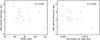 |
Fig. A.1 ASDI speckle attenuation factor at 0.5′′ as a function of the PSF FWHM (left) and the noise level of the raw images (right). |
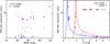 |
Fig. A.2 ASDI self-subtraction factor as a function of the PSF FWHM (left) and the planet flux ratio (right) derived for two separations to the image center. For the right panel, we also represent the theoretical curves for the self-subtraction measured on a diffraction-limited PSF processed in SDI alone (no ADI) as a function of the flux ratio (solid lines). The measurements and the theoretical curve determined at 0.5′′ are shifted horizontally by 1 unit toward the right with respect to the data obtained at 1′′ for the sake of clarity. Also note the point representing HIP 106231 at 0.5′′, which is outside the plot ranges (FWHM = 119 mas, F1/F3b = 0.9, ASDI self-subtraction = 100). |
This appendix completes Sect. 5.3 by analyzing possible correlations of the speckle attenuation and self-subtraction with quantities representative of the observations and/or of the spectral properties of point sources.
Appendix A.1: Properties of the ASDI speckle attenuation
We focus here on possible trends of the ASDI speckle attenuation with observational factors. We test six quantities: the PSF FWHM, the Strehl ratio, the raw noise level (without differential imaging), the coherent energy, the turbulence correlation time, and the seeing. The first three factors are derived directly from the images. The next two parameters are the median of the values estimated by the visible AO wavefront sensor (at a wavelength of 2.17 μm and 0.55 μm, respectively). The last quantity is derived by the DIMM at 0.5 μm. The coherent energy and the Strehl ratio are two methods for determining the quality of the AO correction (Fusco et al. 2004). The coherent energy of the NaCo-corrected images is assessed using the slope measurements of the Shack-Hartmann wavefront sensor. We derive the Strehl ratio as the ratio of the maxima of the measured and theoretical normalized PSF. We find general tendencies with the FWHM and the raw noise level at 0.5′′ in Fig. A.1, where the attenuations are greater for lower values of these parameters. We retrieve a general decreasing trend with the Strehl ratio. We observe the same trends (inverted for the Strehl ratio) with these three factors. This is expected, because these factors are related. We note in Fig. A.1 that the vertical dispersion of the measurements is large for both panels. This could be accounted for by the diversity of the observing conditions (Table 2). At larger separations, we retrieve similar correlations with the FWHM and the raw noise level, but they are less pronounced because the speckle noise is less and less dominant (results not shown). We do not determine correlations with the parameters estimated by the AO system. We discuss the errors on the speckle attenuation and FWHM in Sect. 5.3. The error on the normalized raw noise level is the same as the error on the PSF considered in the manuscript (20%).
Appendix A.2: Dependencies of the ASDI self-subtraction
This quantity depends on both observational and spectral factors (Eq. (3)). We use the FWHM as the parameter that is representative of the observations and the companion flux ratio F1/F3b (Fig. 2) as spectral factor. The F1/F3b ratio is calculated by interpolating the model relation on the mass measured at 5σ. Because the self-subtraction is a function of the angular separation, we present the results for two separations in Fig. A.2. For the FWHM (left panel), we do not see any trends if we consider all the points for each separation.
In contrast, we find that the self-subtraction is strongly correlated with F1/F3b. For F1/F3b ≳ 2 (Teff ≲ 800 K, Fig. 2), it is less than 2. In this panel, we also represent the theoretical curves of the self-subtraction due to SDI alone measured for diffraction-limited PSF. Although the data points include both SDI and ADI attenuations, we note that they follow the theoretical relations quite closely. If we focus on the “peak” of the latter, watching out for the horizontal shift for the curve determined at 0.5′′, we note that the corresponding F1/F3b decreases from a value of 1 at the image center as the separation increases. This feature is accounted for well by a polynomial law of degree 3. At 0.5′′, most measurements are in the regime F1/F3b < 1, which means that the companion is brighter at 1.625 μm than at 1.575 μm. This is the case for Teff ≳ 1000 K (Fig. 2).
The self-subtraction does not show trends with the FWHM for a separation of 1′′. This seems to be inconsistent with Fig. 6, in which we found a correlation of the geometric part of the self-subtraction φ(r) with this parameter. However, unlike φ(r), the ASDI self-subtraction is a degenerated quantity. Thus, we have to distinguish different regimes for the self-subtraction when analyzing possible trends. When F1/F3b is high (≳2), the PSF morphology (FWHM, asymmetries) and chromatic behavior (altered by different spectral filters and by the coronagraph chromaticity) will have little impact on the self-subtraction. We observe in the righthand panel of Fig. A.2 that the measurements are close to the theoretical predictions. In contrast, when F1/F3b ≃ 1, the PSF properties will influence the self-subtraction value. This is confirmed in Fig. A.2, where the discrepancies between the measurements and the theoretical case are greater. If we examine the data measured at 1′′ further in the lefthand panel of Fig. A.2 and analyze the points with small and large self-subtractions separately, we find that the former are not correlated with the FWHM. However, for large self-subtractions, we retrieve a behavior similar to what we obtained for φ(r) (Fig. 6). The errors on the quantities represented in Fig. A.2 are described in Sect. 5.3.
All Tables
All Figures
|
Fig. 1 Spectra (Fλ) of model atmospheres of giant planets for different effective temperatures (colored solid lines, BT-Settl models from Allard et al. 2012). Each spectrum is normalized to its value at 1.6 μm and is vertically shifted by a constant. The transmission of the three SDI filters of NaCo (T1, T2, and T3) are shown in black lines with different styles. Theoretical absorption bands of water and methane are also indicated. The vertical scale is linear. |
| In the text | |
|
Fig. 2 Flux ratio as a function of the effective temperature derived for the NaCo SDI filters (Fig. 1). F1, F2, and F3 refer to the fluxes in the filters at 1.575, 1.600, and 1.625 μm, respectively. The theoretical relations are derived for a given age of 70 Myr, so the surface gravity of the object log (g) is not constant. It increases from 3.75 to 4.75 for the plot range. We also consider the same photometric zeropoint for all the SDI filters. |
| In the text | |
|
Fig. 3 Age-distance diagram of the star sample observed in the NaCo SDI survey. The dashed lines indicate the criteria used for the sample selection (age ≲ 200 Myr and distance ≲ 25 pc). |
| In the text | |
|
Fig. 4 Left: single raw image of a target star provided by the SDI mode of NaCo. The wavelength of the four subimages is from the top right in the anticlockwise direction: 1.575, 1.600, 1.625, and 1.625 μm. The image is thresholded and the scale is logarithmic. Right: flat-field image of the SDI filters (the vertical bars of the filter support are visible in the top half of the image), the double Wollaston prism (which produces the four subimages) and the FQPM (the cross visible in each subimage). The image scale is linear. Both image sizes are 1026 pixels × 1024 pixels, and the field of view of each subimage is 8′′ × 8′′. The cut of the images seen on their left side is due to the position of the field selector on the light beam. Note the inverted tints of both images. |
| In the text | |
|
Fig. 5 Residual noise in the I1 image expressed in contrast with respect to the star after ADI alone (solid lines) and after ASDI (dashed lines). We consider for ASDI the subtraction I13b. We represent the median, best, and worst curves in the survey (colored curves, see text). We account for self-subtraction from ADI for all curves using synthetic planets, but not from SDI for the ASDI curves (see text). |
| In the text | |
|
Fig. 6 Azimuthal mean of the geometrical SDI attenuation factor φ(r) derived for all the observed stars and the I13b subtraction at separations of 0.5, 1, and 2 arcsec (colors) as a function of the FWHM (see text). The dotted lines indicate the values for a diffraction-limited PSF. The solid lines are power-law fitting laws. |
| In the text | |
|
Fig. 7 Differential flux F13b of a planet predicted by the evolutionary model BT-Settl (Allard et al. 2012) as a function of mass for all targets and three separations (rows). The stars are sorted by age, <100 Myr (left column) and ≥100 Myr (right column). The top right part of the right panels shows the curve for HIP 114046, which is a very old star (8 Gyr, Table 1). |
| In the text | |
|
Fig. 8 Signal-to-noise ratio of synthetic planets measured in the images of HIP 118008 after ADI (solid lines) and ASDI (dashed lines) as a function of mass for several separations. The cut-off at low masses is due to the evolutionary model BT-Settl (see text). The horizontal dotted black line indicates the signal-to-noise ratio used to derive the mass sensitivity limits (see text). |
| In the text | |
|
Fig. 9 Detection limits in mass of the survey according to the BT-Settl evolutionary model (Allard et al. 2012) after ADI applied to the I1 image (solid curves) and after ASDI performed for the I13b subtraction (dashed curves). The stars are sorted by increasing age from left to right and from top to bottom. The curves are cut when the minimum mass covered by the evolutionary model is reached (see text). |
| In the text | |
|
Fig. 10 Same as Fig. 9 but for the effective temperature. Note the different vertical scale with respect to Fig. 9. |
| In the text | |
|
Fig. 11 ASDI self-subtraction of point sources as a function of the ASDI speckle attenuation for three angular separations (colors). The points are indicated with different symbols according to the ASDI performance in Fig. 9. The dotted line indicates where the ASDI speckle attenuation equals the ASDI self-subtraction. For the sake of clarity, we do not include the point pertaining to HIP 106231 measured at 0.5′′ (speckle attenuation = 0.9, self-subtraction = 100). |
| In the text | |
|
Fig. 12 ASDI mass gain as a function of the PSF FWHM (left) and the SDI flux ratio of the companion (right) for an angular separation of 1′′. The labels refer to the points with the best mass gains. |
| In the text | |
|
Fig. 13 Detection limits in mass using BT-Settl (Allard et al. 2012) and combining several differential imaging methods (see text) as a function of the projected separation. The left panel represents the results for the stars younger than 100 Myr and the right panel those for older targets. The curves are cut according to the maximum projected separation accessible in the SDI field (see text). |
| In the text | |
|
Fig. 14 Histograms of the mass (left) and effective temperature (right) detectable at 5σ (Fig. 13) for several physical separations. The maximum number of stars is 16 for 10 AU and 15 beyond (see text). |
| In the text | |
|
Fig. A.1 ASDI speckle attenuation factor at 0.5′′ as a function of the PSF FWHM (left) and the noise level of the raw images (right). |
| In the text | |
|
Fig. A.2 ASDI self-subtraction factor as a function of the PSF FWHM (left) and the planet flux ratio (right) derived for two separations to the image center. For the right panel, we also represent the theoretical curves for the self-subtraction measured on a diffraction-limited PSF processed in SDI alone (no ADI) as a function of the flux ratio (solid lines). The measurements and the theoretical curve determined at 0.5′′ are shifted horizontally by 1 unit toward the right with respect to the data obtained at 1′′ for the sake of clarity. Also note the point representing HIP 106231 at 0.5′′, which is outside the plot ranges (FWHM = 119 mas, F1/F3b = 0.9, ASDI self-subtraction = 100). |
| In the text | |
Current usage metrics show cumulative count of Article Views (full-text article views including HTML views, PDF and ePub downloads, according to the available data) and Abstracts Views on Vision4Press platform.
Data correspond to usage on the plateform after 2015. The current usage metrics is available 48-96 hours after online publication and is updated daily on week days.
Initial download of the metrics may take a while.