| Issue |
A&A
Volume 565, May 2014
|
|
|---|---|---|
| Article Number | A46 | |
| Number of page(s) | 11 | |
| Section | Extragalactic astronomy | |
| DOI | https://doi.org/10.1051/0004-6361/201323070 | |
| Published online | 05 May 2014 | |
Heating of the molecular gas in the massive outflow of the local ultraluminous-infrared and radio-loud galaxy 4C12.50
1 Observatoire de Paris, LERMA (UMR 8112), 61 Av. de l’Observatoire, 75014 Paris, France
e-mail: This email address is being protected from spambots. You need JavaScript enabled to view it.
2 Institut de Radio Astronomie Millimétrique, 300 rue de la Piscine, 38406 Saint-Martin d’ Hères, France
3 Istituto di Astrofisica e Planetologia Spaziali, INAF-IAPS, via Fosso del Cavaliere 100, 00133 Roma, Italy
Received: 17 November 2013
Accepted: 13 February 2014
Abstract
We present a comparison of the molecular gas properties in the outflow vs. in the ambient medium of the local prototype radio-loud and ultraluminous-infrared galaxy 4C12.50 (IRAS 13451+1232), using new data from the IRAM Plateau de Bure Interferometer and 30 m telescope and from the Herschel space telescope. Previous H2 (0–0) S(1) and S(2) observations with the Spitzer space telescope had indicated that the warm (~400 K) molecular gas in 4C12.50 is made up of a 1.4( ± 0.2) × 108M⊙ ambient reservoir and a 5.2(±1.7) × 107M⊙ outflow. The new CO(1–0) data cube indicates that the corresponding cold (25 K) H2 gas mass is 1.0(±0.1) × 1010M⊙ for the ambient medium and < 1.3 × 10⁸ M⊙ for the outflow, when using a CO-intensity-to-H2-mass conversion factor α of 0.8 M⊙/(K km s-1 pc2). The combined mass outflow rate is high, 230–800 M⊙/yr, but the amount of gas that could escape the galaxy is low. A potential inflow of gas from a 3.3(±0.3) × 108M⊙ tidal tail could moderate any mass loss. The mass ratio of warm-to-cold molecular gas is ≳30 times higher in the outflow than in the ambient medium, indicating that a non-negligible fraction of the accelerated gas is heated to temperatures at which star formation is inefficient. This conclusion is robust against the use of different α factor values and/or different warm gas tracers (H2 vs. H2 plus CO). With the CO-probed gas mass at least 40 times lower at 400 K than at 25 K, the total warm-to-cold mass ratio is always lower in the ambient gas than in the entrained gas. Heating of the molecular gas could facilitate the detection of new outflows in distant galaxies by enhancing their emission in intermediate rotational number CO lines.
Key words: ISM: jets and outflows / ISM: kinematics and dynamics / line: profiles / galaxies: active / galaxies: nuclei / infrared: galaxies
© ESO, 2014
1. Introduction
Mass accretion events onto black holes (BHs) can release more energy than the binding energy of gas in galaxies (Fabian 2012), and part of this energy can be deposited onto the interstellar medium (ISM) through radiation, accretion-disk winds, and radio jets. The energy carried by these so-called feedback mechanisms can excite or kinematically distort gas on large scales (e.g., over areas of square kiloparsecs; Lípari et al. 2004; Fu & Stockton 2009; Rupke & Veilleux 2011; Westmoquette et al. 2012). It can even affect galaxies outside the active galactic nucleus (AGN) that generated it (e.g., Croft et al. 2006; Cantalupo et al. 2012). The effects of feedback on the evolution of galaxies are most severe if part of the gas is accelerated beyond escape velocity. The high-velocity gas will then be lost to the intergalactic medium. Any star formation associated with it will be quenched. For the remaining gas, star formation will be delayed. The low-velocity gas will cool radiatively, resettle in a disk, and restart its collapse toward the formation of new cores. For these reasons, AGN feedback has been considered as a source of negative feedback, capable of regulating galaxy growth. Positive feedback, i.e., compression of gas leading to an enhancement of star formation, has also been occasionally suggested (e.g., van Breugel et al. 1985; Gaibler et al. 2012; Silk 2013).
AGN feedback, implemented either as a source of heating coupled to the hot gas or as a source of momentum coupled to the cold gas, was included in cosmological simulations to suppress star formation at earlier epochs and to make the predicted number counts of massive present-day galaxies match the observed ones (Granato et al. 2004; Croton et al. 2006; Bower et al. 2006; Somerville et al. 2008; Booth & Schaye 2009; Debuhr et al. 2012). The claim that feedback could change the high-mass end of the local galaxy mass function by more than an order of magnitude has however been contested by Birnboim et al. (2007), Dekel & Birnboim (2008), and Bernardi et al. (2013), who argue that the numbers could be revised downward through, e.g., different stellar population modeling assumptions.
The change in the galaxy mass function by AGN feedback remains to be quantified or constrained by observations. To quantify it, we need to determine the frequency of AGN-driven outflows that can considerably delay or quench star formation in their host galaxies. Even though high-velocity outflows have long been identified in optical and radio data of ionized and neutral atomic gas tracers in local AGN (e.g., Heckman et al. 2000; Rupke et al. 2005; Martin 2005; Morganti et al. 2005; Holt et al. 2008), this research field became particularly appealing thanks to the launch of infrared (IR) space missions (e.g., Herschel) and the improvement on the sensitivity and the spectral range of ground-based mm facilities, which enabled us to probe the molecular gas content of outflows. As the densest ISM component, the molecular gas can contribute considerably to the mass of the entrained gas, if not dominate it. Motions of molecular gas that could be associated with a nuclear outflow have been presented for ~50 local galaxies to date (Sakamoto et al. 2006, 2009; Leon et al. 2007; Feruglio et al. 2010; Fischer et al. 2010; Alatalo et al. 2011; Rangwala et al. 2011; Sturm et al. 2011; Krips et al. 2011; Dasyra & Combes 2011, 2012; Aalto et al. 2012; Tsai et al. 2012; Morganti et al. 2013a; Combes et al. 2013; Spoon et al. 2013; Veilleux et al. 2013; Cicone et al. 2014). Mass measurements of the accelerated gas were presented in around one fifth of the cases and found to be in the range 106–109 M⊙.
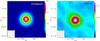 |
Fig. 1 Left: 102 GHz continuum image of 4C12.50 (in units of Jy/beam). Right: continuum-free CO(1–0) line intensity map of 4C12.50 averaged over the –500 km s-1 to 500 km s-1 range, showing extended emission that is offset from the continuum peak (marked with a cross). The contours are at the 3σ levels for this image, i.e., in steps of 0.36 mJy/beam. |
To identify spectral lines with strong outflow signatures and use them for the systematic and efficient detection of new outflows, we need to perform excitation studies of the gas in the flow, motivated by the argument that the AGN feedback could leave both kinematic and excitation signatures on the ISM. Such studies have nonetheless only been presented for a couple of sources. In Mrk 231, Cicone et al. (2012) found no evidence of any strong contribution of shocks on the excitation of outflowing CO molecules at states of low rotational number J: the CO(2–1)/CO(1–0) flux ratio was comparable in the outflow and in the ambient medium.
In this paper, we present evidence of heating of the molecular gas in the outflow of the local radio-loud and ultraluminous-infrared system 4C12.50 (IRAS 13451+1232), i.e., a late-stage merger of two galaxies where the nuclei are separated by 4.4 kpc and surrounded by smaller structures (Batcheldor et al. 2007). A relativistic radio jet with an intrinsic bulk flow speed of at least 0.8c emerges from the system’s west nucleus (Lister et al. 2003). The setup of a radio jet propagating through a gas-rich galaxy, which is rare in the local Universe but common at high redshift (e.g., Sajina et al. 2008; Ivison et al. 2012), makes 4C12.50 an excellent target for studying the properties of the outflowing molecular gas. Moreover, 4C12.50 was the only source in the Spitzer archive for which a warm molecular gas outflow was discovered and characterized. An outflow-related wing was detected in two purely rotational H2 lines, providing the entrained gas excitation temperature and mass (Dasyra & Combes 2011). Cold gas was also discovered in the outflow of 4C12.50 thanks to absorption seen in CO(2–3) with a significant optical deph against the millimeter continuum source (Dasyra & Combes 2012). In this paper, we compare the properties of the gas in the outflow vs. in the ambient medium using new submillimeter and millimeter data, and we discuss the implications of our findings for future searches of massive molecular gas outflows. Throughout our work, we adopt a ΛCDM cosmology with H0 = 70 km s-1 Mpc-1, ΩM = 0.3, and ΩΛ = 0.7.
2. Data
The CO(1–0) observations were carried out with the Plateau de Bure (PdB) Interferometer of the Institut de Radioastronomie Millimétrique (IRAM) as part of the program V028 (PI Dasyra). The data were taken on four different days between September 2011 and January 2012, during which four, five, or six antennae were placed in compact (C, D, or special) configurations. The dual polarization SIS receivers were tuned at a frequency ν of 102.761 GHz, and used with the WIDEX backend. The typical weather conditions were 0.6–2.2′′ of seeing and 2–10 mm of water vapor. Bandpass calibrators (0923+392,1354+195, 3C 84, 3C 279) were observed before our primary target during the first two runs. During the next two runs, they were observed before and after each 22.5 min-long integration on 4C12.50. This change to the observational strategy enabled us to minimize the scatter due to the strong millimeter continuum of 4C12.50 by monitoring changes in the time-variable bandpass solution and thus increasing the accuracy of the subsequent phase and flux calibrations. To perform the last two tasks, we used the default IRAM environment, CLIC1, selecting 4C12.50 itself for the phase calibration and MWC 349 for the flux calibration. The calibrated visibilities of all tracks were merged into a single table, of depth equivalent to 12.5 h of observations with a six-antenna array. A cube of 0.34′′ per spatial pixel was created from this table using the default PdB image reconstruction environment, MAPPING1. Its 1σ noise is 1.1 mJy per beam at a spectral resolution of 5.7 km s-1. The clean 3 mm beam corresponds to an ellipse with semi-major and semi-minor axis of 4.0′′ and 3.8′′, respectively, at a position angle of 14°. We constructed the continuum image by computing the median of all cube planes in the 450 km s-1 to 1250 km s-1 range, and removed it from the entire cube to obtain a continuum-free CO(1–0) line cube (Fig. 1).
Observations at 205.522 GHz targeting the CO(2–1) line were carried out in June 2012 with the IRAM 30 m telescope. The Eight Mixer Receiver (EMIR; Carter et al. 2012) and the Wideband Line Multiple Autocorrelator (WILMA) backend were used for this program. The FTS backend was also connected for repeatability. The data presented here are rather shallow, at 20 min of on-source integration time, taken while the 1.5 mm system temperature varied from 400 to 450 K. The deterioration of the weather conditions prevented the acquisition of more data. The individual scans were examined, stacked, and binned to 47 km s-1 channels within the CLASS environment1.
We followed up 4C12.50 with the PACS (Poglitsch et al. 2010) far-infrared instrument onboard Herschel (Pilbratt et al. 2010) to look for emission from CO molecules that are excited to states of high rotational number. High spectral sampling CO(16–15) observations were carried out for our GT2_lspinogl_6 program in range-spectroscopy mode using chop-nod cycles. To populate the CO spectral line energy distribution (SLED), we combined our data with all PACS range or line spectroscopy data in the Herschel archive that cover the observed-frame wavelengths of CO lines in 4C12.50. For this reason, we examined the blue array data and their parallel red array data in each astronomical observation request (AOR). We found that, in total, information is available for four transitions, CO(33–32), CO(22–21), CO(18–17), and CO(16–15), with integration times of 1.2, 4.0, 1.4, and 2.1 h, respectively. For CO(22−21), this is the total time of the combined OT1_dfarrah_1 and OT1_sveilleu_3 program data. We reduced the data within the Herschel Interactive Processing Environment (HIPE; version 8.3, calibration tree version 32; Ott et al. 2010), by running the default PACS spectrometer pipeline for chopped-line and short-range scans with a wavelength grid oversampling parameter2 of 2. We flagged as outliers all pixel read-outs in emission-line-free wavelengths whose flux exceeded 5σ. Because 4C12.50 is a point source for PACS, we obtained its final spectrum at each wavelength by extracting the spectrum of the central 9.4′′ × 9.4′′ spaxel of each data cube and by multiplying it by the point-source-correction factor in order to recover its full flux. We followed an identical procedure to reduce all other archival PACS observations of 4C12.50 in order to obtain information on its far-infrared dust continuum emission. From this process, we excluded AORS in spectral ranges that suffer from flux leakage from/to other wavelengths, such as <54 μm, 70−74 μm, and 95–105 μm.
3. Results
3.1. CO(1–0) data: gas mass and distribution
The median channel with a CO(1–0) detection in the PdB data cube is at 102.756 GHz, pointing to a redshift z of 0.12179. When adopting this redshift and collapsing the continuum-subtracted cube over the −500 km s-1 to 500 km s-1 velocity range, we find that the CO(1–0) emission is offset from the 3 mm continuum peak and marginally extended (Fig. 1). When examining the data cube within the −500 <V< 500 km s-1 range, we find that the CO(1–0) emission progresses from the east to the west as the velocity increases from negative to positive values (Figs. 2, 3). It peaks at two locations, ~1′′ (or ~2.2 kpc) apart. This emission arises from gas that could be associated with the two main merging nuclei of 4C12.50 (Dasyra et al. 2006a), with an off-center disk forming due to the merger, or with a combination of the above.
A distinct, off-center component is also detected in the central velocity bin of Fig. 3, at ~10 kpc southwest of the main nucleus. An inspection of the data cube at a higher spectral resolution (Fig. 4) reveals that this component has a tidal structure, approaching the main component at systemic velocity. Its distance from the center progressively increases with increasing velocity, until it reaches 12 kpc at ~30 km s-1. The structure has a faint counterpart in the optical (Fig. 5), and it is by far the most gas-rich (and thus dust-rich) of all tidal tails in this system.
The spectra extracted from the data cube are shown in Figs. 6 and 7 for the main component, and Fig. 8 for the tidal tail. Figure 6 reveals an asymmetry in the CO(1–0) emission profile along the east-west axis at sub-beam scales that is likely due to the merger. The profile can also be compatible with absorption of CO and continuum emission by molecules at systemic velocity, such as in Centaurus A (Eckart et al. 1990; Wiklind & Combes 1997).
To find the mass of the H2 gas that is associated with the CO emission shown in Figs. 7 and 8, we computed the product 3.25 × 10⁷ α SCO(1 − 0) ΔV 
 /(1+z)3M⊙, where α is the CO intensity to H2 mass conversion factor, SCO(1 − 0) ΔV is the integrated line flux in Jy km s-1, νobs is the observed CO(1–0) frequency in GHz, and DL is the source luminosity distance in Mpc (Solomon et al. 1997). We adopted an α value of 0.8 M⊙/(K km s-1 pc2), to be consistent with the literature assuming a lower conversion factor for ultraluminous infrared galaxies (ULIRGs) than for the Milky Way (Downes & Solomon 1998).
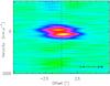 |
Fig. 2 Position-velocity diagram of the continuum-free CO(1–0) emission along the east-west axis, displayed for a velocity resolution of 6 km s-1. The x-axis offset is computed from the radio core location, which is marked with a dashed line. The offset increases (/decreases) toward the west (/east). |
 |
Fig. 3 Continuum-free CO(1–0) line intensity map of 4C12.50, displayed for ~114 km s-1 bins (in the range −315 km s-1 to 369 km s-1). The number in the upperleft corner of each frame corresponds to the bin mean velocity. Contours are plotted at integer multiples of the 5σ level for these images, i.e., in steps of 2.4 mJy/beam. A shift toward the west of the line peak position from negative to positive velocities, as well as a distinct kinematic component near rest-frame velocity are observed. |
 |
Fig. 4 Same as in Fig. 3, but for bins of 17 km s-1 (in the range 0 to 34 km s-1). Contours are plotted at integer multiples of the 3.5σ level for these images, i.e., in steps of 3.3 mJy/beam. |
For the main emission component (Figs. 1, 7), we measured a flux of 18.2 ± 1.5 Jy km s-1. From this flux we calculated a cold H2 gas mass reservoir of 1.0( ± 0.1) × 1010 M⊙. Likewise, the flux in the tidal tail is 0.61 ± 0.04 Jy km s-1 (integrated down to the 1σ level, as shown in Fig. 5). This corresponds to an H2 mass of 3.3( ± 0.3) × 108 M⊙. We thus find that a mass comparable to 1/30th of the main reservoir could be infalling thanks to the tidal tail (see Sect. 4). Because the total CO(1–0) flux in the PdB data agrees within the error with that previously measured in IRAM 30 m telescope data (20 ± 6 Jy km s-1; Dasyra & Combes 2011), we deduce that the interferometer did not miss a significant part of the extended emission.
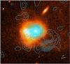 |
Fig. 5 Contours of the CO(1–0) emission of 4C12.50, integrated from 25 km s-1 to 35 km s-1 and plotted over an 7300 Å Hubble Space Telescope ACS image (Batcheldor et al. 2007). The contours start at the 1σ level of the collapsed CO(1–0) image, 0.014 Jy/beam. They are spaced by an equal amount. |
A spatially-unresolved absorption line at −720 km s-1 at the radio core and less than a handful of emission lines at V< − 500 km s-1 or V> 500 km s-1 were seen in the PdB data at ~3–5 root mean square noise (σ) levels. Their widths never exceeded ~80 km s-1. These lines could be real (owing to a small collection of high-velocity clouds in the outflow) or artifacts (due to the varying position and intensity of the mm continuum, which leads to an inadequate removal of the point spread function). A reliable detection of the outflow in CO(1–0) remains to be achieved with higher dynamic range observations. In the rest of this work, we adopt an upper limit of 1.3 × 10⁸ M⊙ for the mass of the cold molecular gas in the outflow. We computed this limit by integrating 3σ over the velocity range that the molecular outflow spans in other wavelengths (−1300 km s-1<V< − 300 km s-1; Dasyra & Combes 2011, 2012). We further assumed that the outflow is spatially unresolved, constrained within our four-kiloparsec-radius beam. Indeed, no evidence of an extended (ionized gas) outflow was found in multi-slit optical spectra of 4C12.50 (Holt et al. 2008, 2011). The neutral atomic gas component of the outflow observed in the radio is found ~150 pc away from the nucleus, at the tip of the southern radio hot spot (Morganti et al. 2013b).
3.2. Higher rotational number CO lines
The IRAM 30 m telescope CO(2–1) data (Fig. 9) have a beam of ~12′′, which comprises all regions seen in emission in the PdB data. The measured CO(2–1) flux3 was 35 (±)6 Jy km s-1, which together with a previously measured CO(3–2) flux of 50 ± 8 Jy km s-1 (Dasyra & Combes 2012), indicates a subthermal excitation of the CO molecules. Their excitation up to J = 3 is identical with that of the gas in the Milky Way, toward the Galactic center, and higher than in the outflow of M82 (Fig. 11; Weiss et al. 2001, 2005).
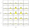 |
Fig. 6 CO(1–0) line profile changes within few arcseconds (i.e., at sub-beam scales) from the position of the radio core in the PdB data. All spectra are plotted in the −1200 km s-1 to 1200 km s-1 velocity range. |
High-J CO emission was not detected with PACS, with a probable exception for the 22−21 transition (Fig. 10): weak (3.5σ) signal was seen at restframe 118.58 μm, which was also seen by Spoon et al. (2013) and Veilleux et al. (2013) in their independent reductions of different sub-sets of the data. For the sake of completeness, we note that a spectrum of 4C12.50 showing no detection of CO lines was also acquired (OT1_pogle01_1) with SPIRE (Griffin et al. 2010). The limits used in this work (Table 1) are based on the wavelength-dependent instrumental sensitivity for the integration time of the SPIRE observations.
By means of a qualitative comparison of the SLED (Fig. 11), we find that the high-J states of CO molecules are considerably less populated in 4C12.50 than those in local prototype AGN in which shock fronts and X-ray-photodissociation regions are likely to contribute to the gas excitation (e.g., NGC 1068 and NGC 6240; Krips et al. 2011; Hailey-Dunsheath et al. 2012; Spinoglio et al. 2012; Meijerink et al. 2013).
3.3. CO spectral line energy distribution fitting: cold vs. warm gas reservoir
To derive fundamental properties of the gas that is probed by our CO observations, we modeled the CO SLED with the radiative transfer code RADEX, assuming for simplicity that the flux that we detected over a line width of ~520 km s-1 originates in a collection of clouds with same average properties and intrinsic line widths of 1 km s-1 (van der Tak et al. 2007). Further assuming that the cosmic microwave background temperature is 3.06 K and that the CO is excited by collisions with hydrogen and helium, we ran a grid of CO column density NCO, CO kinetic temperature Tkin, and H2 volume density nH2 models to find those that best fit our data.
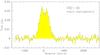 |
Fig. 7 Line profile of the main CO(1–0) emission component in the PdB data. The flux is integrated down to the 1σ level of the integrated CO(1–0) emission (Fig. 1; typically 7–9′′ from the radio core), excluding the emission from the tidal structure, which is shown in Fig. 8. |
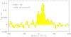 |
Fig. 8 PdB CO(1–0) spectrum of the tidal structure southwest of the merging nuclei of 4C12.50, integrated down to the 1σ flux level of Fig. 5. |
We considered intrinsic column densities in the range 5 × 10¹⁴–5 × 1017 cm-2, corresponding to the beam-averaged CO column density in the chosen velocity step, divided by a filling factor of the beam by the clouds in the range 1–0.001. To compute this beam-averaged column density from the CO(1–0) observations, we used an H2 gas mass of 1.0 × 10¹⁰ M⊙, a CO abundance that is 104 times lower than that of the H2, and we equally divided the mass between 520 velocity bins. Having three unknown parameters and three line luminosity measurements, we obtained an exact solution for the model that best describes the molecular emission from the J = 1, J = 2, and J = 3 upper states. It corresponds to a filling factor of 0.025, a CO kinetic temperature of 25 K, and an H2 volume density of 1.5 × 103 cm-3. In this solution, the CO(1–0)-emitting gas is out of local thermodynamic equilibrium (LTE): the CO(1–0) beam-corrected brightness temperature is 11 K, i.e., ~two times lower than the H2 kinetic temperature. The data of the CO(1–0) and CO(2–1) lines alone are compatible with a temperature of 7 K, for the same volume density but for a higher filling factor (0.092). The data of the CO(1–0) and CO(3–2) lines alone are compatible with a temperature as high as 32 K, again for the same volume density but for a lower filling factor (0.017).
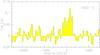 |
Fig. 9 IRAM 30 m telescope data of CO(2–1), comprising all regions where CO(1–0) was detected in the PdB data (i.e., the main component and the tidal structure). |
CO line observations.
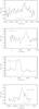 |
Fig. 10 PACS observations of 4C12.50 that cover the wavelengths of high-J CO spectral lines. |
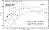 |
Fig. 11 CO SLED of 4C12.50 shown for transitions up to J = 22–21. The CO(22–21) line is seen at 3.5σ levels. Based on our RADEX modeling, the SLED of the three lowest transitions is best fit by gas with a kinetic temperature of 25 K (dashed line). Examples of RADEX models that are consistent with the Herschel data are also shown for gas with a kinetic temperature of 400 K, for a couple of column and volume density combinations (dashed-dotted and dotted lines). The SLEDs of other prototype sources are overplotted for comparison, normalized to LCO(1 − 0)(4C12.50)/LCO(1−0). |
To estimate the maximum warm gas mass that is probed by the CO, we calculated the maximum emission by molecules at high rotational states that is compatible with the observed SLED after fixing Tkin to 400 K. This kinetic temperature is marginally higher than the excitation temperature of the H2 gas seen with Spitzer (374 ± 12 K; Dasyra & Combes 2011). For this computation, our free parameters were the H2 volume density and the CO column density. Our column density grids were expanded to lower values than before. A model fitting the CO(18–17) and CO(22–21) data has an H2 volume density of 2 × 106 cm-3, and a CO column density of 5 × 1013 cm-2 (Fig. 11). The mass of the warm H2 as probed by the CO at 400 K is then equal to 2.5 × 7 M⊙, or 0.0025 times the mass of the cold H2 probed by the CO at 25 K, under the assumption that the emitting areas of the warm and the cold gas are identical. The 400 K gas mass would decrease if the CO(22–21) line luminosity were to be treated as an upper limit. If the warm gas were to be more tenuous, with an H2 volume density of 1 × 105 cm-3, then the CO column density would have to be below 5 × 1014 cm-2 for the CO(7–6) to CO(13–12) luminosity limits to be respected. In that case, the upper limit on the mass of the warm gas would be 2.5 × 8 M⊙. In the likely presence of intermediate Tkin components, the mass estimate will again decrease.
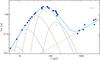 |
Fig. 12 Dust SED of 4C12.50 including continuum measurements from the new IRAM and Herschel data. The modified black body curves (with temperatures between 19 K and 400 K) that best fit the IR/sub-mm data are plotted with dotted lines. The dashed line is a synchrotron-related power law with an exponent of 0.9. The solid line corresponds to the sum of the flux of all components. |
To compare the gas and dust properties in the ambient medium, we produced the dust spectral energy distribution (SED) of 4C12.50 using our Herschel and IRAM continuum flux measurements (from this work, Table 2, Dasyra & Combes 2012) together with data from the literature (Moshir et al. 1990; Steppe et al. 1995; Clements et al. 2010; Ostorero et al. 2010; Trippe et al. 2010; Guillard et al. 2012). The large scatter in the radio data is due to the time variability of the continuum. We fitted the SED by minimizing the χ2 between the observations and a model consisting of multiple modified black body curves and a power law. We parameterized the flux emitted by each modified black body as ![Mathematical equation: \hbox{$(M_{\rm dust}\, \kappa_{\rm abs}[\lambda_0]/D_L^2)\, (\lambda_0/\lambda )^{\beta}\,(2 h \nu ^3/c^2)\, /({\rm e}^{h\nu /kT} -1)$}](/articles/aa/full_html/2014/05/aa23070-13/aa23070-13-eq88.png) , where Mdust is the dust mass at temperature T, κabs [λ0] is the dust absorption coefficient at the reference wavelength λ0, h is the Planck constant, and k is the Boltzmann constant. We opted for a reference wavelength accessible to PACS, 150 μm, and parameter values of β = 2.0 and κabs[150 μm] = 11.6 cm2 gr-1. These parameter values reproduce the absorption coefficient of the Draine (2003)RV = 3.1, Milky Way dust model with an accuracy of 10% in the 70 to 1000 μm range. We limited the temperature of the coldest dust SED component in the range 5–35 K. We also fixed the temperature of another component at 400 K, i.e., at the Tkin of the warm CO SLED component. A χ2 minimization using the IDL MPFIT code indicated that three more components are needed to reproduce the observed SED (Fig. 12). From the SED modeling, we found that the infrared luminosity of 4C12.50 is 2.4( ± 0.1) × 1012L⊙, that the component that best fits the peak of the SED is at T = 40 ± 3 K, and that the component with the lowest temperature is at 19 ± 5 K.
, where Mdust is the dust mass at temperature T, κabs [λ0] is the dust absorption coefficient at the reference wavelength λ0, h is the Planck constant, and k is the Boltzmann constant. We opted for a reference wavelength accessible to PACS, 150 μm, and parameter values of β = 2.0 and κabs[150 μm] = 11.6 cm2 gr-1. These parameter values reproduce the absorption coefficient of the Draine (2003)RV = 3.1, Milky Way dust model with an accuracy of 10% in the 70 to 1000 μm range. We limited the temperature of the coldest dust SED component in the range 5–35 K. We also fixed the temperature of another component at 400 K, i.e., at the Tkin of the warm CO SLED component. A χ2 minimization using the IDL MPFIT code indicated that three more components are needed to reproduce the observed SED (Fig. 12). From the SED modeling, we found that the infrared luminosity of 4C12.50 is 2.4( ± 0.1) × 1012L⊙, that the component that best fits the peak of the SED is at T = 40 ± 3 K, and that the component with the lowest temperature is at 19 ± 5 K.
Continuum fluxes in the infrared and mm range.
The temperatures of the coldest dust SED components thus bracket the kinetic temperature of the cold CO SLED component (25 ± 8 K). The SLED could also be reproduced up to CO(3-2) by a combination of two gas components with temperatures lower than or equal to those of the dust (e.g., 7 K and 40 K). Collisions with the ambient ISM could thus suffice to explain the excitation of the bulk of the CO molecules. A jet-induced shock does not have to be invoked instead.
4. Discussion
4.1. Heating of the accelerated molecular gas with respect to the ambient medium
The results presented in Sect. 3 raise the question of how the excitation properties of the accelerated molecular gas compare with those of the dynamically relaxed gas. From the Spitzer data, we know that the outflow has a warm component, carrying 5.2 × 10⁷ M⊙ of H2 molecules at ~400 K (Dasyra & Combes 2011). From a CO(2–3) absorption line that is due to clouds obscuring the millimeter continuum and moving at −950( ± 90) km s-1, we know that colder molecules do exist in the outflow (Dasyra & Combes 2012). Only a lower limit could be placed on their mass from the CO(2–3) data, because the absorption only probes the few lines of sight toward the millimeter continuum. The millimeter continuum is less extended than the radio continuum due to the steep power law that describes the emission from the jet lobes (Krichbaum et al. 1998, 2001, 2008), and the radio continuum is in its turn constrained to around ten hot spots with a radius of a few parsec each (Morganti et al. 2013b). The bulk of the cold entrained CO is thus likely to be found in lines of sight without a millimeter background, and it should be detected in emission. Its non-detection in our CO(1–0) PdB data now enables us to place an upper limit of 1.3 × 10⁸ M⊙ on the mass of cold entrained H2 gas.
Putting all numbers together, we find that the mass ratio of warm (400 K) to cold (25 K) H2 gas in the outflow is >0.40. For the ambient medium, containing 1.0 × 10¹⁰ M⊙ of H2 molecules at 25 K and 1.4 × 10⁸ M⊙ of H2 molecules at ~400 K (Sect. 3; Dasyra & Combes 2011), the same ratio is only 0.014. A major result of this work is thus that the mass ratio of warm-to-cold H2 gas is at least 29 times higher in the outflow than in the ambient medium.
Taking into account that a non-negligible fraction of the mid-infrared H2 emission could be due to gas that was accelerated by the front shock but that is not accounted for in the outflow due to its low velocity, we conclude that the discrepancy in the warm-to-cold mass ratio could increase. Contrarily, adding the mass of the warm ambient H2 probed by high-J CO lines to the mass of the warm ambient H2 measured by Spitzer could decrease this discrepancy. Still, it would not alter our conclusion. Adding 2.5 × 7M⊙ of gas distributed in a dense 400 K component (in agreement with the high-J CO emission in Fig. 11) would lead to a warm-to-cold H2 mass ratio that is ≥24 times higher in the outflow than in the ambient medium. Even adding the maximum amount of 400 K gas that is compatible with the CO SLED, 2.5 × 8 M⊙, would lead to a ratio that is ≥10 times higher in the outflow than in the ambient medium. Likewise, our conclusion is robust against the use of another α factor, or the use of different α factors for the entrained and ambient gas (see, e.g., Papadopoulos et al. 2012). The latter choice can be justified because the CO intensity to H2 mass conversion scales with Tkin-1(nH2)1/2 for virialized clouds (Maloney et al. 1988; Weiss et al. 2001). Figure 13, showing the dependence of the warm-to-cold H2 mass ratio on the α factor, indicates that there is no combination of acceptable α and warm gas mass values that could make the ratio in the ambient medium agree with the one in the outflow. Instead, the ratio in the outflow is at least 3−30 times higher than in the ambient medium in the entire parameter space.
Our results constitute direct evidence that the accelerated molecular gas can be heated4 to the point where star formation is inefficient. The accelerated and heated gas can be detected even though the cooling timescales can be considerably shorter than the outflow propagation timescales (Guillard et al. 2012), possibly thanks to the enhancement of turbulence on individual-cloud scales (Nesvadba et al. 2011). Papadopoulos et al. (2008) and Ogle et al. (2010) previously attributed the overall strong emission by CO molecules in states of intermediate rotational number and by H2 molecules in states of low rotational number to shock excitation by radio jets.
4.2. Impact of the outflow on the galaxy
The outflow could affect the future evolution of 4C12.50 via gas heating or gas expulsion. While the effects of heating are uncertain, we observe that the feedback mechanism has not had enough time to reach and excite a large fraction of the CO reservoir.
To test the role of gas expulsion, we computed the mass outflow rate, Ṁout, which is equal to MoutVoutd-1 . We revised the flow rate of warm gas presented in Dasyra & Combes (2011) from 130 M⊙ yr-1 to 230 M⊙ yr-1, using identical values for the outflow velocity Vout (640 km s-1) and mass Mout (5.2 × 10⁷ M⊙), but assuming that the entrained gas is within a distance d of 150 pc from the radio core (Morganti et al. 2013b). The flow of cold gas could carry up to 570 M⊙ yr-1, under the assumption that the entrained CO and the entrained H2 have the same average velocity. This assumption does not conflict with the CO(2−3) detection at −950 km s-1 (Dasyra & Combes 2012), which only probes the motions of some outflowing clouds: those situated between us and the radio core. For both gas phases, the total mass flow rate is in the range 230–800 M⊙ yr-1.
However, only a part of this gas could be lost to the intergalactic medium. The escape velocity at 150 pc from the western nucleus of 4C12.50 is 700 km s-1, when assuming an isothermal sphere distribution for the visible baryonic matter and when using a stellar velocity dispersion of 170 km s-1 and a half-light radius of 2.6 kpc (Dasyra et al. 2006a). The escape velocity will increase to 800 km s-1 when the mass in the eastern nucleus of 4C12.50 is accounted for. From the H2 velocity distribution in the Spitzer data, less than 30% of the gas could be lost to the intergalactic medium. Most of the accelerated and heated gas will fountain back to a disk within a few dynamical timescales. The maximum mass loss rate would be ≲240 M⊙/yr, and the minimum depletion timescale of the reservoir ≳4 × 10⁷ yrs. The depletion timescale could increase further and exceed the typical values for AGN duty cycles when the mass in the dark matter halo(s) is taken into account.
Any gas expulsion could be moderated or counteracted by a potential inflow of gas from the southern tidal tail. At the projected distance of the tail, ~10 kpc, the escape velocity from the visible baryonic matter is in the range 200–300 km s-1, i.e., higher than the typical rotational velocities of spiral arms. Given that the line-of-sight velocity of the tidal tail is <40 km s-1, gas could be captured and fed to the western nucleus.
We thus postulate that both gas expulsion and heating are likely to temporarily delay but unlikely to entirely suppress star formation in 4C12.50.
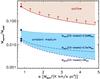 |
Fig. 13 Warm-to-cold gas mass ratio as a function of the α conversion factor. The circle shows the ratio’s lower limit in the outflow for α = 0.8 M⊙/(K km s-1 pc2). The solid line shows how this lower limit decreases as α approaches values thought appropriate for the Milky Way. This curve brackets the range of all acceptable Mwarm/Mcold values in the outflow (hatched area), under the assumption that the 400 K outflowing gas fraction probed by the CO is negligible compared to the fraction probed by the H2. For the ambient medium, the measuredratio (triangles) and its dependence on α (non-solid lines) are given for different warm gas content scenarios: when only the mass of the 400 K H2 gas directly seen by Spitzer is used (dashed line) and when the mass of another CO-based 400 K gas component is added. The dashed-dotted line uses an additional mass of 2.5 × 7 M⊙ distributed in clouds of 2 × 106 cm-3 (as in the dashed-dotted CO SLED component in Fig. 11). The dotted line instead uses an additional mass of 2.5 × 8 M⊙ distributed in clouds of 1 × 105 cm-3 (as in the dotted CO SLED component in Fig. 11). This line constrains the upper range of acceptable Mwarm/Mcold values in the ambient medium (solid area). |
4.3. Driving mechanism of the outflow
Power and momentum arguments are typically invoked for evaluating the outflow driver. The flow kinetic luminosity can be computed from the product  . For the Mout, Vout, and d values discussed in Sect. 4.2, the kinetic luminosity of the warm entrained gas that is probed by the H2 is 3 × 1043 erg s-1. Adding the maximum amount of cold outflowing gas that could be probed by the CO would place the kinetic luminosity upper limit to 1 × 1044 erg s-1. The luminosity radiated by the outflowing gas in the purely rotational H2 lines, 4 × 1041 erg s-1 (Dasyra & Combes 2011), is negligible with respect to the outflow kinetic luminosity. The luminosity radiated in CO lines is even lower than that radiated in H2 lines.
According to Veilleux et al. (2009), half of the infrared luminosity of this source can be ascribed to its AGN and half to its starburst, with an uncertainty of ~50% on either fraction. The dust-based star-formation-rate estimate is then 400 M⊙/yr (Kennicutt 1998). The power released by supernovae (SN) is 1044 erg s-1, under the assumption that for every hundred solar masses forming there is one SN (e.g., in the Kroupa 2001, initial mass function context), ejecting material with a kinetic energy of 1051 erg. This energy is insufficient to drive the flow unless a very large fraction (30–100%) of it is converted into the outflow kinetic luminosity.
The luminosity of the AGN, like that of the starburst, is estimated to be 5 × 1045 erg s-1. The force exerted to the gas by radiation pressure is then 5 to 18 times lower than the outflow momentum rate, when the latter is approximated by the product  (Combes et al. 2013). The momentum rate boost needed for the gas acceleration could occur with the aid of energy-conserving gas expansion or multiple photon scatterings in high optical depth regions (Faucher-Giguère & Quataert 2012). For these mechanisms, the compact-source geometry of the AGN is advantageous.
The AGN jet constitutes a generous power source, capable of driving the flow. The radio cavity kinetic luminosity is estimated from its 178 MHz flux to be 3 × 1045 erg s-1 (Guillard et al. 2012). The most significant argument in favor of the radio jet remains the location of the H I outflow at the tip of the southern radio hot spot (Morganti et al. 2013b). The young age of the jet, limited to <105 yrs (Lister et al. 2003), could explain why only a small amount of the CO is affected by the feedback.
4.4. Implications for future observations
Recent hydrodynamic simulations indicate that gas heating could be common in AGN outflows: the effects of jets and radiation-driven ultra-fast winds on the ISM can be comparable only 104–105 years after the onset of the feedback activity (Wagner & Bicknell 2011; Wagner et al. 2013), when both mechanisms drive bubbles of similar flow structure and dynamics.
If heating of the accelerated molecular gas is common, then the detection of outflows could be easier in intermediate-J CO lines than in low-J CO lines, facilitating the discovery of outflows in the distant Universe: at z ~ 1 or higher, for example, ALMA could probe outflows of comparable mass to those presently detected at 100 Mpc with the PdB. Moreover, the acquisition of infrared data alongside millimeter data could be valuable for the systematic discovery and reliable mass determination of outflows. With ALMA operating in full-array mode in about two years and with the James Webb Space Telescope coming up beyond 2018, these goals will be achievable for most systems of interest in the local Universe. At 100 Mpc, ALMA is designed to detect 5 × 10⁵M⊙ outflows of 10 K gas in CO(1–0). The JWST is designed to reach the same limit for the ~100 K gas probed by H2(0–0)S(1). For typical outflow radial extents of a few hundred pc, this common detection threshold corresponds to an outflow rate of ~1 M⊙ yr-1, comparable to the star formation rate in local spirals.
5. Conclusions
We used IRAM PdB, 30 m telescope, and Herschel Space Telescope data to study the content, excitation, and kinematic properties of the molecular gas in the outflow and in the ambient medium of a local prototype radio-loud, ultraluminous-infrared galaxy, 4C12.50 (also known as IRAS 13451+1232). We specifically looked for gas heating and expulsion signatures, i.e., characteristics of the two feedback-related processes that can delay star formation. Combining new and previous observations, we found evidence that both processes are taking place, and we drew the following main conclusions.
-
The CO(1–0) emission spatially con-sists of a newly discovered tidal tail, which extends outto 12 kpc southwest of the nucleus, and amain component, which is marginally resolved withinthe beam radius (4.2 kpc). A shift in thelocation of the maximum emission with velocity indi-cates that the main component could be tracing eithertwo merging nuclei or a rotating disk. Its reservoir con-tains 1.0( ± 0.1) × 1010 M⊙ of cold H2 gas for α = 0.8 M⊙/(K km s-1 pc2).
-
The CO SLED, which is primarily tracing the ambient gas in 4C12.50, is very similar with that of the Milky Way gas for low-J numbers. Fitting of the CO SLED with RADEX indicates that the gas mass probed by CO molecules at 400 K is less than 0.025 times the gas mass probed by CO molecules at 25 K. Likewise, the H2 gas mass probed by CO molecules at 400 K is less than 1.7 times the mass of the 400 K gas probed by the purely rotational H2 lines in the mid-infrared.
-
In the outflow, the mass of the cold (25 K) H2 gas is <1.3( ± 0.1) × 108 M⊙, i.e., at most twice as high as the mass of the warm (400 K) H2 gas emitting in the mid-infrared. By combining the H2-based mass flow rate measurement from the mid-infrared data, 230 M⊙/yr, with the CO-based mass flow rate upper limit from the mm data, 570 M⊙/yr, we conclude that the feedback mechanism(s) could be accelerating up to 800 M⊙/yr of molecular gas for an outflow radius of 150 pc.
-
A small fraction of the outflowing gas (<30% when ignoring dark matter) could escape the system and be lost to the intergalactic medium. Any mass loss could be moderated or counteracted by a potential inflow of gas from the tidal tail containing 3.3( ± 0.3) × 108 M⊙ of cold H2. The star formation in the host of 4C12.50 is likely to be delayed, but not entirely suppressed by the feedback.
-
The mass ratio of warm-to-cold H2 gas is elevated in the outflow with respect to the ambient medium by a factor of ≳30 for α = 0.8 M⊙/(K km s-1 pc2). The conclusion that the accelerated molecular gas is heated is robust against two main sources of uncertainty: the chosen α conversion factor and the mass of the warm gas probed by the CO. While the discrepancy will be lower for higher values of either parameter, there is no combination of acceptable parameter values that could make the warm-to-cold gas mass ratio in the ambient medium reach the ratio in the outflow.
-
A scenario in which outflows could be probed by a different CO SLED than the rest of the ISM is likely. It remains to be tested with submillimeter observations.
The differences between the spectra obtained by running the default pipeline and the spectra obtained by running the routines for an alternative flux calibration based on the telescope background are within the given error bars.
The width of the CO(2–1) line in the 30 m telescope data, 390 ± 68 km s-1, is lower and more uncertain than that of the CO(1–0) line in the PdB data. The uncertainty is due to the sinusoidal baseline in the single-dish data due to standing waves related to the bright continuum of 4C12.50. It does not necessarily translate into a flux loss. For comparison, see the different line shape but identical line flux of CO(1–0) obtained with the PdB array and the 30 m telescope (Dasyra & Combes 2012).
Heating of the molecular gas, leading to excitation at high rotational states, could be one of the reasons that absorption of the mm continuum by outflowing molecules is not (reliably) detected in CO(0–1) in the PdB data, while it was detected in CO(2–3) in the single-dish data. Alternatively, absorption in CO(0–1) may not be seen if it is diluted in CO(1–0) emission. A similar scenario may not hold for CO(2–3) and CO(3–2) depending, e.g., on the size and the geometry of the emitting regions. Changes with time in the relative position of the foreground clouds and the background source leading to changes in the covering factor, or changes with time in the millimeter continuum flux could also justify this result.
Acknowledgments
K.M.D. thanks F. Casoli, O. La Marle, and M. Lozach for making this project possible by means of a French Space Agency (Centre National d’ Études Spatiales; CNES) fellowship. Our work is based on data obtained with the facilities of IRAM, which is supported by INSU/CNRS (France), MPG (Germany), and IGN (Spain), and on data obtained with the Herschel Space Telescope, which is an ESA space observatory with science instruments provided by European-led principal investigator consortia and with important participation from NASA.
References
- Aalto, S., Garcia-Burillo, S., Muller, S., et al. 2012, A&A, 537, A44 [NASA ADS] [CrossRef] [EDP Sciences] [Google Scholar]
- Alatalo, K., Blitz, L., Young, L. M., et al. 2011, ApJ, 735, 88 [NASA ADS] [CrossRef] [Google Scholar]
- Batcheldor, D., Tadhunter, C., Holt, J., et al. 2007, ApJ, 661, 70 [NASA ADS] [CrossRef] [Google Scholar]
- Bernardi, M., Meert, A., Sheth, R. K., et al. 2013, MNRAS, 436, 697 [NASA ADS] [CrossRef] [Google Scholar]
- Birnboim, Y., Dekel, A., & Neistein, E. 2007, MNRAS, 380, 339 [NASA ADS] [CrossRef] [Google Scholar]
- Booth, C. M., & Schaye, J. 2009, MNRAS, 398, 53 [NASA ADS] [CrossRef] [Google Scholar]
- Bower, R. G., Benson, A. J., Malbon, R., et al. 2006, MNRAS, 370, 645 [NASA ADS] [CrossRef] [Google Scholar]
- Cantalupo, S., Lilly, S. J., & Haehnelt, M. G. 2012, MNRAS, 425, 1992 [NASA ADS] [CrossRef] [Google Scholar]
- Carter, M., Lazareff, B., Maier, D., et al. 2012, A&A, 538, A89 [NASA ADS] [CrossRef] [EDP Sciences] [Google Scholar]
- Cicone, C., Feruglio, C., Maiolino, R., et al. 2012, A&A, 543, A99 [NASA ADS] [CrossRef] [EDP Sciences] [Google Scholar]
- Cicone, C., Maiolino, R., Sturm, E., et al. 2014, A&A, 562, A21 [NASA ADS] [CrossRef] [EDP Sciences] [Google Scholar]
- Combes, F., Garcia-Burillo, S., Casasola, V., et al. 2013, A&A, 558, A124 [NASA ADS] [CrossRef] [EDP Sciences] [Google Scholar]
- Clements, D. L., Dunne, L, & Eales, S. 2010, MNRAS, 403, 274 [NASA ADS] [CrossRef] [Google Scholar]
- Croft, S., van Breugel, W., de Vries, W., et al. 2006, ApJ, 647, 1040 [NASA ADS] [CrossRef] [Google Scholar]
- Croton, D. J., Springel, V., White, S. D. M., et al., 2006, MNRAS, 367, 864 [NASA ADS] [CrossRef] [Google Scholar]
- Dasyra, K. M., & Combes, F. 2011, A&A, 533, L10 [NASA ADS] [CrossRef] [EDP Sciences] [Google Scholar]
- Dasyra, K. M., & Combes, F. 2012, A&A, 541, L7 [NASA ADS] [CrossRef] [EDP Sciences] [Google Scholar]
- Dasyra, K. M., Tacconi, L. J., Davies, R. I., et al. 2006a, ApJ, 638, 745 [NASA ADS] [CrossRef] [Google Scholar]
- Dasyra, K. M., Tacconi, L. J., Davies, R. I., et al. 2006b, ApJ, 651, 835 [NASA ADS] [CrossRef] [Google Scholar]
- Debuhr, J., Quataert, E., & Ma, C.-P. 2012, MNRAS, 420, 2221 [NASA ADS] [CrossRef] [Google Scholar]
- Dekel, A., & Birnboim, Y. 2008, MNRAS, 383, 119 [NASA ADS] [CrossRef] [Google Scholar]
- Downes, D., & Solomon, P. M. 1998, ApJ, 507, 615 [NASA ADS] [CrossRef] [Google Scholar]
- Draine, B. T. 2003, ARA&A, 41, 241 [NASA ADS] [CrossRef] [Google Scholar]
- Eckart, A., Cameron, M., Genzel, R., et al. 1990, ApJ, 365, 522 [NASA ADS] [CrossRef] [Google Scholar]
- Fabian, A. C. 2012, ARA&A, 50, 455 [NASA ADS] [CrossRef] [Google Scholar]
- Faucher-Giguère, C.-A., & Quataert, E. 2012, MNRAS, 425, 605 [NASA ADS] [CrossRef] [Google Scholar]
- Feruglio, C., Maiolino, R., Piconcelli, E., et al. 2010, A&A, 518. L155 [Google Scholar]
- Fischer, J., Sturm, E., González-Alfonso, E., et al. 2010, A&A, 518, L41 [NASA ADS] [CrossRef] [EDP Sciences] [Google Scholar]
- Fu, H., & Stockton, A. 2009, ApJ, 690, 953 [NASA ADS] [CrossRef] [Google Scholar]
- Gaibler, V., Khochfar, S., Krause, M., & Silk, J. 2012, MNRAS, 425, 438 [NASA ADS] [CrossRef] [Google Scholar]
- Golombek, D., Miley, G. K., & Neugebauer, G. 1988, AJ, 95, 26 [NASA ADS] [CrossRef] [Google Scholar]
- Granato, G. L., De Zotti, G., Silva, L., Bressan, A., & Danese, L. 2004, ApJ, 600, 580 [Google Scholar]
- Griffin, M. J., Abergel, A., Abreu, A., et al. 2010, A&A, 518, L3 [Google Scholar]
- Guillard, P., Ogle, P., Emonts, B., et al. 2012, ApJ, 747, 95 [NASA ADS] [CrossRef] [Google Scholar]
- Hailey-Dunsheath, S., Sturm, E., Fischer, J., et al. 2012, ApJ, 755, 57 [NASA ADS] [CrossRef] [Google Scholar]
- Heckman, T. M., Lehnert, M. D., Strickland, D. K., & Armus, L. 2000, ApJS, 129, 493 [NASA ADS] [CrossRef] [MathSciNet] [Google Scholar]
- Holt, J., Tadhunter, C. N., & Morganti, R. 2008, MNRAS, 387, 639 [NASA ADS] [CrossRef] [Google Scholar]
- Holt, J., Tadhunter, C. N., Morganti, R., & Emonts, B. H. C. 2011, MNRAS, 410, 1527 [NASA ADS] [Google Scholar]
- Ivison, R. J., Smail, I., Amblard, A., et al. 2012, MNRAS, 425, 1320 [NASA ADS] [CrossRef] [Google Scholar]
- Kennicutt, R. C. 1998, ApJ, 498, 541 [NASA ADS] [CrossRef] [Google Scholar]
- Krichbaum, T. P., Alef, W., Witzel, A., et al. 1998, A&A, 329, 873 [NASA ADS] [Google Scholar]
- Krichbaum, T. P., Graham, D., Witzel, A., et al. 2001, ASP Conf., 250, 184 [NASA ADS] [Google Scholar]
- Krichbaum, T. P., Lee, S. S., Lobanov, A. P., et al. 2008, ASP Conf., 386, 186 [NASA ADS] [Google Scholar]
- Krips, M., Martín, S., Eckart, A., et al. 2011, ApJ, 736, 37 [NASA ADS] [CrossRef] [Google Scholar]
- Kroupa, P. 2001, MNRAS, 322, 231 [NASA ADS] [CrossRef] [Google Scholar]
- Leon, S., Eckart, A., Laine, S., et al. 2007, A&A, 473, 747 [NASA ADS] [CrossRef] [EDP Sciences] [Google Scholar]
- Lípari, S., Mediavilla, E., Diaz, R. J., et al. 2004, MNRAS, 348, 369 [NASA ADS] [CrossRef] [Google Scholar]
- Lister, M. L., Kellermann, K. I., Vermeulen, R. C., et al. 2003, ApJ, 584, L135 [NASA ADS] [CrossRef] [Google Scholar]
- Maloney, P., & Black, J. H. 1988, ApJ, 325, 389 [NASA ADS] [CrossRef] [Google Scholar]
- Martin, C. L. 2005, ApJ, 621, 227 [Google Scholar]
- Meijerink, R., Kristensen, L. E., Weiss, A., et al. 2013, ApJ, 762, L16 [NASA ADS] [CrossRef] [Google Scholar]
- Morganti, R., Tadhunter, C. N., & Oosterloo, T. A. 2005, A&A, 444, L9 [NASA ADS] [CrossRef] [EDP Sciences] [Google Scholar]
- Morganti, R., Frieswijk, W., Oonk, R. J. B., Oosterloo, T., & Tadhunter, C. 2013a, A&A, 552, L4 [NASA ADS] [CrossRef] [EDP Sciences] [Google Scholar]
- Morganti, R., Fogasy, J., Paragi, Z., et al. 2013b, Science, 341, 1082 [NASA ADS] [CrossRef] [Google Scholar]
- Moshir, M., Kopan, G., Conrow, T., et al. 1990, BAAS, 22, 1325 [NASA ADS] [Google Scholar]
- Nesvadba, N., Boulanger, F., Lehnert, M., et al. 2011, A&A, 536, L5 [NASA ADS] [CrossRef] [EDP Sciences] [Google Scholar]
- Ogle, P., Boulanger, F., & Guillard, P. 2010, ApJ, 724, 1193 [NASA ADS] [CrossRef] [Google Scholar]
- Ostorero, L., Moderski, R., Stawarz, L., et al. 2010, ApJ, 715, 1071 [NASA ADS] [CrossRef] [Google Scholar]
- Ott, S. 2010, ASP Conf. Ser., 434, 139 [Google Scholar]
- Papadopoulos, P. P., Kovacs, A., Evans, A. S., & Barthel, P. 2008, A&A, 491, 483 [NASA ADS] [CrossRef] [EDP Sciences] [Google Scholar]
- Papadopoulos, P. P., van der Werf, P., Xilouris, E., Isaak, K., & Gao, Y. 2012, ApJ, 751, 10 [NASA ADS] [CrossRef] [Google Scholar]
- Pilbratt, G. L., Riedinger, J. R., Passvogel, T., et al. 2010, A&A, 518, L1 [CrossRef] [EDP Sciences] [Google Scholar]
- Poglitsch, A., Waelkens, C., Geis, N., et al. 2010, A&A, 518, L2 [NASA ADS] [CrossRef] [EDP Sciences] [Google Scholar]
- Rangwala, N., Maloney, P. R., & Glenn, J. 2011, ApJ, 743, 94 [NASA ADS] [CrossRef] [Google Scholar]
- Rupke, D. S., Veilleux, S., & Sanders, D. B. 2005, ApJ, 632, 751 [Google Scholar]
- Rupke, D. S. N., & Veilleux, S. 2011, ApJ, 729, L27 [NASA ADS] [CrossRef] [Google Scholar]
- Sajina, A., Yan, L., Lutz, D., et al. 2008, ApJ, 683, 659 [NASA ADS] [CrossRef] [Google Scholar]
- Sakamoto, K., Ho, P. T. P., & Peck, A. B. 2006, ApJ, 644, 862 [NASA ADS] [CrossRef] [Google Scholar]
- Sakamoto, K., Aalto, S., & Wilner, D. J. 2009, ApJ, 700, L104 [NASA ADS] [CrossRef] [Google Scholar]
- Sanders, D. B., & Mirabel, I. F. 1996, ARA&A, 34, 749 [NASA ADS] [CrossRef] [Google Scholar]
- Silk, J. 2013, ApJ, 772, 112 [NASA ADS] [CrossRef] [Google Scholar]
- Solomon, P. M., Downes, D., Radford, S. J. E., & Barrett, J. W. 1997, ApJ, 478, 144 [NASA ADS] [CrossRef] [Google Scholar]
- Somerville, R. S., Hopkins, P. F., Cox, T. J., et al. 2008, MNRAS, 391, 481 [NASA ADS] [CrossRef] [Google Scholar]
- Spinoglio, L., Pereira-Santaella, M., Busquet, G., et al. 2012, ApJ, 758, 108 [NASA ADS] [CrossRef] [Google Scholar]
- Spoon, H. W. W., Farrah, D., Lebouteiller, V., et al. 2013, ApJ, 775, 127 [NASA ADS] [CrossRef] [Google Scholar]
- Steppe, H., Jeyakumar, S., Saikia, D. J., & Salter, C. J. 1995, A&AS, 113, 409 [NASA ADS] [Google Scholar]
- Sturm, E., González-Alfonso, E., Veilleux, S., et al. 2011, ApJ, 733, L16 [NASA ADS] [CrossRef] [Google Scholar]
- Trippe, S., Neri, R., Krips, M., et al. 2010, A&A, 515, A40 [NASA ADS] [CrossRef] [EDP Sciences] [Google Scholar]
- Tsai, A.-L., Matsushita, S., Kong, A. K. H., et al. 2012, ApJ, 752, 38 [NASA ADS] [CrossRef] [Google Scholar]
- van Breugel, W., Filippenko, A. V., Heckman, T., & Miley, G. 1985, ApJ, 293, 83 [NASA ADS] [CrossRef] [Google Scholar]
- van der Tak, F. F. S., Black, J. H., Schöier, F. L., Jansen, D. J., & van Dishoeck, E. F. 2007, A&A, 468, 627 [NASA ADS] [CrossRef] [EDP Sciences] [Google Scholar]
- Veilleux, S., Rupke, D., Kim, D. C., et al. 2009, ApJS, 182, 628 [NASA ADS] [CrossRef] [Google Scholar]
- Veilleux, S., Meléndez, M., Sturm, E., et al. 2013, ApJ, 776, 27 [NASA ADS] [CrossRef] [Google Scholar]
- Wagner, A. Y., & Bicknell, G. V. 2011, ApJ, 728, 29 [NASA ADS] [CrossRef] [Google Scholar]
- Wagner, A. Y., Umemura, M., & Bicknell, G. V. 2013, ApJ, 763, L18 [NASA ADS] [CrossRef] [Google Scholar]
- Weiss, A., Neininger, N., Hüttemeister, S., & Klein, U. 2001, A&A, 365, 571 [NASA ADS] [CrossRef] [EDP Sciences] [Google Scholar]
- Weiss, A., Walter, F., & Scoville, N. Z. 2005, A&A, 438, 533 [NASA ADS] [CrossRef] [EDP Sciences] [Google Scholar]
- Westmoquette, M. S., Clements, D. L., Bendo, G. J., & Khan, S. A. 2012, MNRAS, 424, 416 [NASA ADS] [CrossRef] [Google Scholar]
- Wiklind, T., & Combes, F. 1997, A&A, 324, 51 [NASA ADS] [Google Scholar]
All Tables
All Figures
|
Fig. 1 Left: 102 GHz continuum image of 4C12.50 (in units of Jy/beam). Right: continuum-free CO(1–0) line intensity map of 4C12.50 averaged over the –500 km s-1 to 500 km s-1 range, showing extended emission that is offset from the continuum peak (marked with a cross). The contours are at the 3σ levels for this image, i.e., in steps of 0.36 mJy/beam. |
| In the text | |
|
Fig. 2 Position-velocity diagram of the continuum-free CO(1–0) emission along the east-west axis, displayed for a velocity resolution of 6 km s-1. The x-axis offset is computed from the radio core location, which is marked with a dashed line. The offset increases (/decreases) toward the west (/east). |
| In the text | |
|
Fig. 3 Continuum-free CO(1–0) line intensity map of 4C12.50, displayed for ~114 km s-1 bins (in the range −315 km s-1 to 369 km s-1). The number in the upperleft corner of each frame corresponds to the bin mean velocity. Contours are plotted at integer multiples of the 5σ level for these images, i.e., in steps of 2.4 mJy/beam. A shift toward the west of the line peak position from negative to positive velocities, as well as a distinct kinematic component near rest-frame velocity are observed. |
| In the text | |
|
Fig. 4 Same as in Fig. 3, but for bins of 17 km s-1 (in the range 0 to 34 km s-1). Contours are plotted at integer multiples of the 3.5σ level for these images, i.e., in steps of 3.3 mJy/beam. |
| In the text | |
|
Fig. 5 Contours of the CO(1–0) emission of 4C12.50, integrated from 25 km s-1 to 35 km s-1 and plotted over an 7300 Å Hubble Space Telescope ACS image (Batcheldor et al. 2007). The contours start at the 1σ level of the collapsed CO(1–0) image, 0.014 Jy/beam. They are spaced by an equal amount. |
| In the text | |
|
Fig. 6 CO(1–0) line profile changes within few arcseconds (i.e., at sub-beam scales) from the position of the radio core in the PdB data. All spectra are plotted in the −1200 km s-1 to 1200 km s-1 velocity range. |
| In the text | |
|
Fig. 7 Line profile of the main CO(1–0) emission component in the PdB data. The flux is integrated down to the 1σ level of the integrated CO(1–0) emission (Fig. 1; typically 7–9′′ from the radio core), excluding the emission from the tidal structure, which is shown in Fig. 8. |
| In the text | |
|
Fig. 8 PdB CO(1–0) spectrum of the tidal structure southwest of the merging nuclei of 4C12.50, integrated down to the 1σ flux level of Fig. 5. |
| In the text | |
|
Fig. 9 IRAM 30 m telescope data of CO(2–1), comprising all regions where CO(1–0) was detected in the PdB data (i.e., the main component and the tidal structure). |
| In the text | |
|
Fig. 10 PACS observations of 4C12.50 that cover the wavelengths of high-J CO spectral lines. |
| In the text | |
|
Fig. 11 CO SLED of 4C12.50 shown for transitions up to J = 22–21. The CO(22–21) line is seen at 3.5σ levels. Based on our RADEX modeling, the SLED of the three lowest transitions is best fit by gas with a kinetic temperature of 25 K (dashed line). Examples of RADEX models that are consistent with the Herschel data are also shown for gas with a kinetic temperature of 400 K, for a couple of column and volume density combinations (dashed-dotted and dotted lines). The SLEDs of other prototype sources are overplotted for comparison, normalized to LCO(1 − 0)(4C12.50)/LCO(1−0). |
| In the text | |
|
Fig. 12 Dust SED of 4C12.50 including continuum measurements from the new IRAM and Herschel data. The modified black body curves (with temperatures between 19 K and 400 K) that best fit the IR/sub-mm data are plotted with dotted lines. The dashed line is a synchrotron-related power law with an exponent of 0.9. The solid line corresponds to the sum of the flux of all components. |
| In the text | |
|
Fig. 13 Warm-to-cold gas mass ratio as a function of the α conversion factor. The circle shows the ratio’s lower limit in the outflow for α = 0.8 M⊙/(K km s-1 pc2). The solid line shows how this lower limit decreases as α approaches values thought appropriate for the Milky Way. This curve brackets the range of all acceptable Mwarm/Mcold values in the outflow (hatched area), under the assumption that the 400 K outflowing gas fraction probed by the CO is negligible compared to the fraction probed by the H2. For the ambient medium, the measuredratio (triangles) and its dependence on α (non-solid lines) are given for different warm gas content scenarios: when only the mass of the 400 K H2 gas directly seen by Spitzer is used (dashed line) and when the mass of another CO-based 400 K gas component is added. The dashed-dotted line uses an additional mass of 2.5 × 7 M⊙ distributed in clouds of 2 × 106 cm-3 (as in the dashed-dotted CO SLED component in Fig. 11). The dotted line instead uses an additional mass of 2.5 × 8 M⊙ distributed in clouds of 1 × 105 cm-3 (as in the dotted CO SLED component in Fig. 11). This line constrains the upper range of acceptable Mwarm/Mcold values in the ambient medium (solid area). |
| In the text | |
Current usage metrics show cumulative count of Article Views (full-text article views including HTML views, PDF and ePub downloads, according to the available data) and Abstracts Views on Vision4Press platform.
Data correspond to usage on the plateform after 2015. The current usage metrics is available 48-96 hours after online publication and is updated daily on week days.
Initial download of the metrics may take a while.