| Issue |
A&A
Volume 565, May 2014
|
|
|---|---|---|
| Article Number | A6 | |
| Number of page(s) | 14 | |
| Section | Interstellar and circumstellar matter | |
| DOI | https://doi.org/10.1051/0004-6361/201322687 | |
| Published online | 18 April 2014 | |
Exploring GLIMPSE bubble N107
Multiwavelength observations and simulations
1
Astronomical Institute of the Academy of Sciences of the Czech
Republic, v. v. i., Bočnì II
1401/1a, 141 31
Praha 4, Czech
Republic
e-mail:
This email address is being protected from spambots. You need JavaScript enabled to view it.
2
Department of Physics and Astronomy, University of Calgary, 2500
University Dr NW, Calgary, Alberta,
T2N 1N4,
Canada
3
Dominion Radio Astrophysical Observatory,
PO Box 248, Penticton, B.C.
V2A 6J9,
Canada
4
Okanagan College, 1000 KLO Road, Kelowna, B.C.
V1Y 4X8,
Canada
Received:
16
September
2013
Accepted:
11
February
2014
Abstract
Context. Bubble N107 was discovered in the infrared emission of dust in the plane of the Milk y Way Galaxy observed by the Spitzer Space Telescope (GLIMPSE survey: l ≈ 51.̊0, b ≈ 0.̊1). The bubble represents an example of shell-like structures found all over the Milky Way Galaxy.
Aims. We aim to analyse the atomic and molecular components of N107, as well as its radio continuum emission. With the help of numerical simulations, we aim to estimate the bubble’s age and other parameters that cannot be derived directly from observations.
Methods. From the observations of the H i (I-GALFA) and 13CO (GRS) lines we derive the bubble’s kinematical distance and masses of the atomic and molecular components. With the algorithm DENDROFIND, we decompose molecular material into individual clumps. From the continuum observations at 1420 MHz (VGPS) and 327 MHz (WSRT), we derive the radio flux density and the spectral index. With the numerical code ring, we simulate the evolution of stellar-blown bubbles similar to N107.
Results. The total H i mass associated with N107 is 5.4 × 10³ M⊙. The total mass of the molecular component (a mixture of cold gasses of H2, CO, He, and heavier elements) is 1.3 × 10⁵ M⊙, from which 4.0 × 10⁴ M⊙ is found along the bubble border. We identified 49 molecular clumps distributed along the bubble’s border, with the slope of the clump mass function of −1.1. The spectral index of −0.30 of a strong radio source located apparently within the bubble indicates nonthermal emission, hence part of the flux probably originates in a supernova remnant, not yet catalogued. The numerical simulations suggest N107 is most likely less than 2.25 Myr old. Since the first supernovae explode only after 3 Myr or later, no supernova remnant should be present within the bubble. It may be explained if there is a supernova remnant in the direction towards the bubble, however not associated with it.
Key words: ISM: bubbles / ISM: clouds / ISM: supernova remnants / HII regions
© ESO, 2014
1. Introduction
Bubble N107 (SIMBAD: CPA2006 N107) is one of the largest bubbles in the catalogue by Churchwell et al. (2006). This catalogue is based on the infrared observations made with the Spitzer Space Telescope (GLIMPSE survey, Benjamin et al. 2003) and contains more than 300 bubbles found in the interstellar medium (ISM) near the Galactic plane. The catalogue was later expanded by Simpson et al. (2012) to more than 5000 bubbles, which were identified by a community of over 35 000 volunteers. These bubbles, with typical radii less than 10 pc, are examples of shell-like structures, features found in the ISM all over our Galaxy. Other examples are H i shells in catalogues by Heiles (1979, 1984) and Ehlerová & Palouš (2005) with sizes up to 3500 pc, or dusty loops discovered in the IRAS full-sky survey by Kiss et al. (2004) and Könyves et al. (2007).
The varying sizes and masses of these structures suggest different mechanisms responsible for their creation. These mechanisms, which do not have to act solely, include
-
1.
feedback from massive (OB) stars: radiation, winds andsupernovae (see refs. below);
-
2.
infall of high-velocity clouds into the Galactic disc (e.g. Heiles 1984; Tenorio-Tagle & Bodenheimer 1988; Ehlerová & Palouš 1996);
-
3.
energy and mass inserted by gamma-ray bursts (e.g. Efremov et al. 1998, 1999; Loeb & Perna 1998); and
-
4.
turbulence (Dib & Burkert 2005).
Bubble N107, like most of the GLIMPSE bubbles, is probably a result of stellar feedback (Churchwell et al. 2006; Deharveng et al. 2010), which may follow three different models:
-
1.
An expanding H ii region, assuming radia-tive heating and ionisation of hydrogen by UV photons from amassive star (Kahn 1954; Oort &Spitzer 1955; Spitzer 1978).The pressure inside the H ii region is higher thanthe ambient neutral medium, so the H ii regionexpands and collects the neutral material in an expanding shell.
-
2.
A wind-blown bubble, supposing that energy is released via stellar winds (Castor et al. 1975; Weaver et al. 1977). Such a bubble, formed around a massive star, can be divided into several layers: an innermost layer, where the wind is freely expanding up to a layer of shocked stellar wind, where its kinetic energy is thermalised. This layer of the shocked wind is followed by a layer of swept up ISM, which in later stages of evolution is mainly atomic and molecular.
-
3.
A supernova explosion, supposing an abrupt energy input into the ISM, producing an expanding shell/remnant (Chevalier 1974, and references therein).
These different models of stellar feedback were also discussed by Tenorio-Tagle & Bodenheimer (1988), Ehlerová & Palouš (1996), and Efremov et al. (1999).
The shell-like structures can trigger star formation, since they consist of a layer of cold and dense material. In the so-called collect-and-collapse scenario (Elmegreen & Lada 1977; Elmegreen 1994; Whitworth et al. 1994), the shell breaks into fragments and creates a new generation of stars. Radiation driven implosion (Duvert et al. 1990; Lefloch & Lazareff 1994) considers the compression of preexisting condensations (globules) by the pressure of the ionised gas. A brief review of these and other triggering mechanisms is given in a study of GLIMPSE bubbles by Deharveng et al. (2010).
In this paper, we present a multiwavelength study of one of the largest GLIMPSE bubbles,
N107, which lies in the central plane of the Galactic disc
( ,
,  ). A multiwavelength, colour picture
of N107 is shown in Fig. 1.
). A multiwavelength, colour picture
of N107 is shown in Fig. 1.
The paper is organised in the following way: in Sect. 2, we complement the Spitzer infrared observations with H i line observations from the I-GALFA survey (Koo et al. 2010), 13CO (J = 1−0) line observations from the GRS survey (Jackson et al. 2006), and radio continuum observations at 1420 and 327 MHz from the VGPS (Stil et al. 2006) and WSRT (Taylor et al. 1996) surveys. From the line observations, we derive the bubble’s LSR1 radial velocity (RV), kinematical distance and masses of the molecular and atomic components. From the radio continuum observations, we derive the flux densities and corresponding spectral indices of two radio sources lying apparently inside the bubble. In Sect. 3, we use a recently published algorithm DENDROFIND (Wünsch et al. 2012) to decompose the molecular gas associated with the bubble into individual clumps and derive the slope of the clump mass function. In Sect. 4, we use the numerical code ring (Palouš 1990; Ehlerová & Palouš 1996) to simulate the bubble’s evolution in order to estimate its age, energy input, and the size and mass of the molecular cloud from which the bubble evolved. Finally, a discussion and conclusions are presented in Sects. 5 and 6.
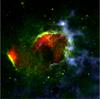 |
Fig. 1 Bubble N107 – false colour multiwavelength image. The 24 μm continuum (red) is dominated by the emission of very small dust grains heated by a nearby massive star. The 8 μm continuum (green) is dominated by the emission of PAHs, large molecules found within molecular clouds. The CO line (blue) is integrated over the radial velocities between 38.5 km s-1 and 47.6 km s-1 and traces the cold gas of molecular clouds. The distinct red-green structure seen in the lower-left in the direction of the bubble’s opening is probably not related to the bubble, since the radial velocity of the associated molecular material (≈60 km s-1) differs significantly from the radial velocity of the N107 complex (≈43 km s-1). |
2. Observation of Bubble N107
2.1. Data sources
The Galactic Legacy Infrared Mid-Plane Survey Extraordinaire (GLIMPSE, Benjamin et al. 2003) and A 24 and 70 Micron Survey of
the Inner Galactic Disk with MIPS (MIPSGAL, Carey et al.
2009) are two complementary infrared surveys mapping the Galactic disc with the
Spitzer Space Telescope. GLIMPSE used the Infrared Array Camera (IRAC)
which has four channels centred around 3.6, 4.5,
5.8, and 8.0 μm, for which the point
response function FWHM2 is between
 and
and
 . MIPSGAL used the Multiband Imaging
Photometer for Spitzer (MIPS) with a broadband channel centred around
24 μm, for
which the point spread function FWHM is 6″.
. MIPSGAL used the Multiband Imaging
Photometer for Spitzer (MIPS) with a broadband channel centred around
24 μm, for
which the point spread function FWHM is 6″.
The Inner-Galaxy ALFA Low-Latitude H i Survey (I-GALFA, Koo et al. 2010) is part of a large project called GALFA-H i
(Peek et al. 2011) that plans to map the
entire sky observable by the Arecibo Observatory in the H i line. The FWHM beam
size of the Arecibo telescope at 1420
MHz is  with the GALFA-H i radial
velocity channel width of 0.184 km
s-1. The data are provided in FITS3 cubes of the brightness temperature Tb. The
single-channel standard deviation of the Gaussian noise σnoise is about
0.25 K.
with the GALFA-H i radial
velocity channel width of 0.184 km
s-1. The data are provided in FITS3 cubes of the brightness temperature Tb. The
single-channel standard deviation of the Gaussian noise σnoise is about
0.25 K.
The Galactic Ring Survey (GRS, Jackson et al.
2006) is a 13CO (J = 1−0) survey focused
on the Galactic molecular ring. The survey used the FCRAO 14 m telescope, with a FWHM beam
size of 46″ and a radial
velocity channel width of 0.21 km
s-1. The data are provided in FITS cubes of the antenna
temperature  , with a
typical noise
, with a
typical noise  . We
converted the data to the main-beam brightness temperature
. We
converted the data to the main-beam brightness temperature
 and
and
 , where
ηMB =
0.48 is the main beam efficiency (value suggested by Jackson et al. 2006).
, where
ηMB =
0.48 is the main beam efficiency (value suggested by Jackson et al. 2006).
The VLA Galactic Plane Survey (VGPS, Stil et al. 2006) is a 1420 MHz continuum and H i line survey of the Galactic disc based on the interferometric observations done with the Karl G. Jansky Very Large Array (VLA). We use only the continuum observations since data from I-GALFA are available with significantly lower noise for the H i. The FWHM beam size is 1′ and the Gaussian noise is 0.3 K for the continuum observations.
The Westerbork Synthesis Radio Telescope survey (WSRT, Taylor et al. 1996) is a 327
MHz continuum survey of the Galactic plane that uses the WSRT
interferometer in the Netherlands. The FWHM resolution is 1′ × (1′ /
sinδ) in the right ascension and declination
(δ)
directions, respectively. This yields for N107 (δ ≈ 16°) the FWHM resolution of
 . The median Gaussian noise is
2.5 mJy /
beam.
. The median Gaussian noise is
2.5 mJy /
beam.
The UKIRT Infrared Deep Sky Survey (UKIDSS) is defined in Lawrence et al. (2007); UKIDSS uses the United Kingdom Infrared Telescope (UKIRT) Wide Field Camera (WFCAM, Casali et al. 2007) and a photometric system described in Hewett et al. (2006). The pipeline processing and science archive are described in Irwin et al. (2004) and Hambly et al. (2008). We used data from the 7th data release.
2.2. Dust component
The bubble’s outline is most prominent in the 8 μm maps from the GLIMPSE survey, where it was
discovered by Churchwell et al. (2006) who derived
its basic properties: mean position of ,
; mean radius of
 , and a mean thickness of
 . Most emission at 8 μm comes from the bubble
edges, forming a ring-like structure. The 8
μm channel is dominated by the emission of
polycyclic aromatic hydrocarbons (PAHs; Draine
2003; Reach et al. 2006, Fig. 1; Pavlyuchenkov et al. 2013). These PAHs, which are
destroyed in the ionised regions, trace the photodissociation regions (PDRs), edges of
molecular clouds illuminated by the UV radiation from a massive star. The UV radiation
pervades the PDRs and excites the PAHs found there.
. Most emission at 8 μm comes from the bubble
edges, forming a ring-like structure. The 8
μm channel is dominated by the emission of
polycyclic aromatic hydrocarbons (PAHs; Draine
2003; Reach et al. 2006, Fig. 1; Pavlyuchenkov et al. 2013). These PAHs, which are
destroyed in the ionised regions, trace the photodissociation regions (PDRs), edges of
molecular clouds illuminated by the UV radiation from a massive star. The UV radiation
pervades the PDRs and excites the PAHs found there.
A Counterpart emission at 24 μm was observed in MIPSGAL (Carey et al. 2009). Unlike the 8 μm continuum, emission at 24 μm fills part of the bubble’s interior. The 24 μm continuum is dominated by the emission of very small grains – dust grains larger than PAHs – heated by a nearby massive star (Pavlyuchenkov et al. 2013).
A dark hole is present in the south-western part of the bubble’s interior. Almost no emission from dust and also no emission of 13CO or H i (see below) is observed there. Figure 1 shows a multiwavelength, colour picture of N107 composed of the 8 μm and 24 μm continuum emission and the 13CO line emission integrated over the radial velocities from 38.5 km s-1 to 47.6 km s-1.
2.3. Atomic component
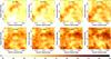 |
Fig. 2 Brightness temperature maps of the H i line in several velocity channels. An outline of bubble N107 as given in the catalogue of Churchwell et al. (2006) is marked with the dashed grey circle. The channels 41.0 km s-1 and 41.9 km s-1 show morphology very similar to that of the 8 μm emission. |
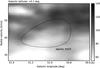 |
Fig. 3 Brightness temperature of the H i line in an l −
v diagram: a cut through
|

We searched the H i data cubes by eye for features possibly associated with bubble N107. An H i shell, morphologically similar to N107, is located around the central LSR radial velocity of 43 km s-1. We note that an incomplete ring of CO clumps is present at similar radial velocities (see Sect. 2.4). The H i emission is located along the bubble edges, protruding outside farther than the CO emission, forming an atomic envelope of the whole structure. Maps of the H i brightness temperature in several velocity channels are shown in Fig. 2.
Figure 3 shows a map of the Galactic longitude versus radial velocity (l-v diagram). The front wall is very faint, located at a radial velocity of ≈34 km s-1. The back wall is more distinct, located at a radial velocity of ≈50 km s-1. Between these radial velocities, a hole can be seen inside the bubble. The relative expansion velocity of the front versus back wall is ≈16 km s-1.
In order to measure the H i mass associated with the bubble, we define the
following 3D aperture (aperture 1, see also Fig. 4,
left panel): radius two times that of N107, 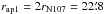 , and the radial velocity channels
from 32.7 km s-1 to
52.0 km s-1
inclusive. All the pixels lying within this aperture contribute to the measured H i
mass.
, and the radial velocity channels
from 32.7 km s-1 to
52.0 km s-1
inclusive. All the pixels lying within this aperture contribute to the measured H i
mass.
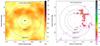 |
Fig. 4 Apertures for measuring the mass associated with bubble N107. The pixels lying within the apertures contribute to the measured masses. The dashed circles mark bubble N107 as was identified in the 8 μm emission by Churchwell et al. (2006). Left: H i line emission at 42.8 km s-1. The innermost circle (BG) is the region we used to derive the background emission. Right: 13CO line emission at 42.8 km s-1. We used two apertures to measure the molecular mass. Aperture 1 is the same as that for measuring the H i mass, while aperture 2 is smaller and covers only the immediate vicinity of the bubble. |
To derive the mass of the neutral hydrogen, we use the optically thin limit of H i
line radiative transfer. Then, the H i column density NH i
can be computed from the formula (Rohlfs & Wilson
1996)  (1)where Tb is the
observed brightness temperature of the H i gas and, in our case of an I-GALFA
data cube, the integral takes the form of a sum over a set of pixels with dv = 0.184 km
s-1.
(1)where Tb is the
observed brightness temperature of the H i gas and, in our case of an I-GALFA
data cube, the integral takes the form of a sum over a set of pixels with dv = 0.184 km
s-1.
The Galactic H i emission has a strong background component. To estimate it, we assume that the bubble’s interior is evacuated, so the H i emission observed apparently near the bubble centre is due to this H i background, not associated with the bubble. We defined another 3D aperture with the radius half that of the N107 and the radial velocity channels from 39.1 km s-1 to 43.7 km s-1 (see Fig. 4). This aperture encloses a volume in the central part of the bubble. The mean Tb within this region is 72 K, which we adopt as the H i background component and subtract it before computing the mass.
Furthermore, in the process of mass derivation, we need to know the distance to N107. We also consider the 13CO emission (see below) and we adopt the central radial velocity of 42.8 km s-1. The Galactic rotation model of Brand & Blitz (1993) gives two kinematical distances for that radial velocity: 3.6 kpc and 7.1 kpc. We adopt the near one of 3.6 kpc, which yields the bubble mean radius of 11.9 pc (11.4′). The near distance is favoured by the estimated virial masses of the molecular clumps found along the bubble borders. For the far distance of 7.1 kpc, we got 22 of 49 clumps with supervirial masses, while for the near distance of 3.6 kpc, we got only 2 clumps with virial masses above 1 (clumps 7 and 21 in Table 2). We note that Churchwell et al. (2006) suggest distances of 4.7/6.0 kpc. They use the same rotation model as we do, but with a less reliable determination of the radial velocity obtained from the observation of coincident H ii regions. They also advocate the near kinematical distance.
To estimate the uncertainty of the measured mass, we use the standard Taylor formula,
 (2)where f is the measured value (in
our case the H i mass) and σf is its uncertainty,
which is derived from uncertainties σxi
of variables xi on which
f depends.
(2)where f is the measured value (in
our case the H i mass) and σf is its uncertainty,
which is derived from uncertainties σxi
of variables xi on which
f depends.
The resulting H i mass associated with N107, i.e. the total H i mass within aperture 1 after subtracting the background, is 5.4 × 10³ M⊙. The major sources of uncertainty are the distance to N107 and the background emission. Assuming the distance uncertainty of 10% (0.36 kpc) and the background uncertainty of 1 K, the total H i mass uncertainty is about 20%, i.e. 1 × 10³ M⊙.
2.4. Molecular component
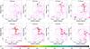 |
Fig. 5 Brightness temperature maps of the 13CO (J = 1 − 0) emission in several velocity channels in degrees Kelvin. An outline of bubble N107 as given in the catalogue of Churchwell et al. (2006) is marked with the dashed grey circle. |
Around the radial velocity of 43 km s-1, CO emission is present along the bubble borders. Maps of the CO emission (Fig. 5) show that CO gas forms clumps, which are distributed in a ring-like structure along the edges of the bubble, protruding outside. Almost no emission comes from the interior. Around the radial velocity of 48 km s-1, the CO emission merges with another complex of molecular clouds, while in the channels below 38 km s-1, CO emission vanishes.
To measure the associated molecular mass, we use two 3D apertures (see Fig. 4, right panel). Aperture 1 is same as that for measuring
the H i mass. Aperture 2 is smaller, with radius
 , radial velocity channels from
38.8 km s-1 to
46.9 km s-1
inclusive and covers only the immediate vicinity of the bubble, i.e. only the mass
accumulated in the expanding shell. We note that to compare the observation and
simulations, we use the molecular mass found within aperture 2. We treat the radiative
transfer in the line of 13CO (J = 1−0), described in
Rohlfs & Wilson (1996). First, we derive
the optical depth,
, radial velocity channels from
38.8 km s-1 to
46.9 km s-1
inclusive and covers only the immediate vicinity of the bubble, i.e. only the mass
accumulated in the expanding shell. We note that to compare the observation and
simulations, we use the molecular mass found within aperture 2. We treat the radiative
transfer in the line of 13CO (J = 1−0), described in
Rohlfs & Wilson (1996). First, we derive
the optical depth, ![Mathematical equation: \begin{equation} \label{eq_tau_13co} \tau = -\ln \left[ 1 - \frac{T_\mathrm{b}}{T_0} \left\{ \left[ \mathrm{e}^{T_0/T_{\mathrm{ex}}} - 1 \right]^{-1} - \left[ \mathrm{e}^{T_0/T_{\mathrm{CMB}}} - 1 \right]^{-1} \right\}^{-1} \right], \end{equation}](/articles/aa/full_html/2014/05/aa22687-13/aa22687-13-eq95.png) (3)where Tex is the
excitation temperature, which we assume to be 20 K; Tb is the brightness temperature of the
CO line; TCMB = 2.7
K is the temperature of the cosmic microwave background and
(3)where Tex is the
excitation temperature, which we assume to be 20 K; Tb is the brightness temperature of the
CO line; TCMB = 2.7
K is the temperature of the cosmic microwave background and
 (4)where h is the Planck constant;
k is the
Boltzmann constant; and f =
110 GHz is the 13CO (J = 1−0) line frequency.
Assuming local thermodynamical equilibrium, characterised by a single excitation
temperature Tex, we can compute the
13CO column density from the formula (Rohlfs & Wilson 1996)
(4)where h is the Planck constant;
k is the
Boltzmann constant; and f =
110 GHz is the 13CO (J = 1−0) line frequency.
Assuming local thermodynamical equilibrium, characterised by a single excitation
temperature Tex, we can compute the
13CO column density from the formula (Rohlfs & Wilson 1996) ![Mathematical equation: \begin{equation} \label{eq_n_13co} \frac{N_{\element[][13]{CO}}}{\mathrm{cm}^{-2}} = 2.6 \times 10^{14} \frac{T_\mathrm{ex}}{1-\mathrm{e}^{-T_0/T_\mathrm{ex}}} \int \tau(v)\,\mathrm{d}v, \end{equation}](/articles/aa/full_html/2014/05/aa22687-13/aa22687-13-eq103.png) (5)where, in our case of
the GRS data cube, dv = 0.21
km s-1 and the integral becomes a sum over a desired range
of pixels. From the 13CO column density, the H2 column density is derived
assuming the abundance (Binney & Merrifield
1998) NH2 = 6.5 ×
105N13CO.
Finally, the total mass of the molecular matter mmol is computed using the standard
solar hydrogen abundance X,
(5)where, in our case of
the GRS data cube, dv = 0.21
km s-1 and the integral becomes a sum over a desired range
of pixels. From the 13CO column density, the H2 column density is derived
assuming the abundance (Binney & Merrifield
1998) NH2 = 6.5 ×
105N13CO.
Finally, the total mass of the molecular matter mmol is computed using the standard
solar hydrogen abundance X,  (6)and mH2
is the mass in the form of the molecular hydrogen. We note that we use term molecular
matter or molecular mass to refer to the matter found in molecular clouds, i.e. a mixture
of H2, He, CO, and
trace amounts of other molecules, elements, and dust. The distance to N107
(3.6 kpc) is discussed above
in Sect. 2.3.
(6)and mH2
is the mass in the form of the molecular hydrogen. We note that we use term molecular
matter or molecular mass to refer to the matter found in molecular clouds, i.e. a mixture
of H2, He, CO, and
trace amounts of other molecules, elements, and dust. The distance to N107
(3.6 kpc) is discussed above
in Sect. 2.3.
The total molecular mass within aperture 1 is 1.3 × 10⁵ M⊙, from which 9.8 × 10⁴ M⊙ is in the form of H2, the rest in helium and heavier elements. The total molecular mass within aperture 2 (in the expanding shell only) is 4.0 × 10⁴ M⊙, from which 2.9 × 10⁴ M⊙ is in the form of H2. The major source of uncertainty is the 13CO abundance. We used NH2 = 6.5 × 10⁵N13CO (Binney & Merrifield 1998). Observations and models show, however, that the abundance varies for different clouds and also depends on the physical conditions inside individual clumps (Sonnentrucker et al. 2007; Visser et al. 2009; Wilson 1999). Another source of the uncertainty we consider is the distance to N107. Using Eq. (2) and assuming the 13CO abundance uncertainty of 20% and the distance uncertainty of 10% (0.36 kpc), the uncertainty of the molecular masses given above is about 30%.
2.5. Radio continuum and spectral index
Since an H ii region was identified in the direction of the bubble (Paladini et al. 2003, region 576) and because the 24 μm emission is also present inside the bubble, we expected to observe its radio continuum counterpart.
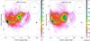 |
Fig. 6 Radio continuum emission associated with bubble N107. The bubble is denoted by the grey dashed circle in the centre. Overlaid are four elliptical apertures (A, B, C, D) used to measure the radio fluxes. The grey dashed ellipse in the upper right (labelled BG) is the region used for measuring the background. Left: emission at 1420 MHz/21 cm from the VGPS survey. Right: emission at 327 MHz/92 cm from the WSRT survey. We note blurring in the direction of declination (top-left-to-bottom-right), caused by the larger beam size (lower resolution) in the declination direction. |
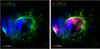 |
Fig. 7 Comparison of the VGPS radio continuum at 1420 MHz/21 cm (blue) with the 8 μm (green) and 24 μm (red) emission. Left: 1420 MHz and 8 μm emission. The radio continuum follows the bubble outline and fills part of its interior. Right: same as left with added 24 μm emission. Inside the bubble, the radio continuum is well correlated with the 24 μm emission, except for the eastern part, where the 24 μm emission is absent and only the radio continuum is observed. |
Both the VGPS (1420 MHz) and
WSRT (327 MHz) surveys show a
distinct diffuse radio source in the direction of the bubble. The source is located
towards the eastern (left) part of the bubble interior, slightly below the area where the
24 μm
emission is strongest (see Fig. 6). Except for this
source, the bubble interior is filled with much fainter radio emission. Another diffuse
radio source is present farther east of the bubble
( , b ≈ 0°). This source is
associated with a complex of molecular material found at radial velocities of about
60 km s-1, so it
is probably not associated with the bubble. Figure 7
shows a comparison of the VGPS radio continuum with the emission at 8 μm and 24 μm. Inside the bubble,
the radio continuum follows the bubble outline defined by the PAHs emission at
8 μm. In
the northern (top) and western (right) part, the radio continuum is mixed with the
emission of very small grains at 24
μm, while in the eastern part (left), the
24 μm
emission vanishes and only the radio continuum is observed.
, b ≈ 0°). This source is
associated with a complex of molecular material found at radial velocities of about
60 km s-1, so it
is probably not associated with the bubble. Figure 7
shows a comparison of the VGPS radio continuum with the emission at 8 μm and 24 μm. Inside the bubble,
the radio continuum follows the bubble outline defined by the PAHs emission at
8 μm. In
the northern (top) and western (right) part, the radio continuum is mixed with the
emission of very small grains at 24
μm, while in the eastern part (left), the
24 μm
emission vanishes and only the radio continuum is observed.
We measured the radio flux densities in four regions: two located towards the bubble
interior – defined by apertures A and B – and two located outside the bubble – defined by
apertures C and D (Fig. 6). Aperture A covers the
distinct source in the eastern part of the bubble (source “A”), while aperture B covers
the faint emission in its western (right) part (source “B”). Aperture C covers part of the
fainter emission outside the bubble (source “C”) and aperture D covers the distinct radio
source located eastwards outside the bubble (source “D”). We subtracted a background
derived from flux within an aperture covering a relatively homogeneous region free of
visible radio sources (Fig. 6). Then we used the two
fluxes at 1420 and
327 MHz to derive the
spectral index α for both sources A and B, 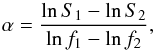 (7)where S1 and
S2 are the fluxes at frequencies
f1 and f2. We note that
the theoretical spectral index for a classical H ii region in the optically thin
limit is −0.1 (Condon & Ransom 2010), although the usually
observed values are around 0
or more (Rohlfs & Wilson 1996; Kellermann & Verschuur 1988). In contrast to
H ii regions, the mean observed spectral index of supernova remnants is
−0.5 (average value in the
catalogue of Green 2009). The measured flux
densities and the derived spectral indices are presented in Table 1.
(7)where S1 and
S2 are the fluxes at frequencies
f1 and f2. We note that
the theoretical spectral index for a classical H ii region in the optically thin
limit is −0.1 (Condon & Ransom 2010), although the usually
observed values are around 0
or more (Rohlfs & Wilson 1996; Kellermann & Verschuur 1988). In contrast to
H ii regions, the mean observed spectral index of supernova remnants is
−0.5 (average value in the
catalogue of Green 2009). The measured flux
densities and the derived spectral indices are presented in Table 1.
The spectral index of source A of −0.3 suggests a nonthermal (synchrotron) contribution to the received radio flux: a supernova remnant. No known supernova remnant is associated, yet, with that radio source. For source B, the spectral index of ≈0 suggests a thermal origin of the flux: a classical H ii region. The spectral indices of sources C (−0.2) and D (−0.1) suggest that part of their emission is also nonthermal.
Radio continuum flux densities and spectral indices for apertures A, B, C, and D.
3. Analysis of molecular clumps
We decomposed the molecular ring associated with N107 into individual molecular clumps with the program DENDROFIND, described in the appendix of Wünsch et al. (2012). DENDROFIND processes data cubes, typically position-position-velocity data cubes of the brightness temperature Tb, and outputs a list of molecular clumps organised in a hierarchical structure, which can be represented by a dendrogram (Rosolowsky et al. 2008). In our case, the data cube is a cutout of the 13CO GRS data and has two spatial dimensions (Galactic longitude, Galactic latitude) and one radial velocity dimension. Each clump consists of a dense core surrounded by a less dense molecular envelope. The core is observed as a local Tb peak. DENDROFIND is controlled by four parameters: Nlevels sets the number of steps by which it goes through the data cube when searching for clump peaks; Npxmin sets the minimal number of pixels which can form a clump; Tcutoff sets the minimal Tb which is still considered a signal, pixels with lower Tb are discarded; dTleaf sets the minimal height of a local peak to be considered a clump’s core; a higher dTleaf will merge more clumps. Parameters Tcutoff and dTleaf are designed to be set to a value of ≈3 × the noise level. We ran DENDROFIND with the parameters Nlevels = 1000, Npixmin =5, and Tcutoff = dTleaf = 1.0 ≈ 3σnoise, where σnoise ≈ 0.34 K is the estimated standard deviation of the Gaussian noise found within our N107 cutout of the 13CO GRS data. We note that this value is slightly greater then the typical value of the entire GRS of 0.27 K given in the paper of Jackson et al. (2006).
Molecular clumps associated with bubble N107.
In order to select only the clumps associated with bubble N107, we took only those clumps
whose cores lie within the aperture 2 used for measuring the total molecular mass (Sect.
2.4). Table 2
lists the identified molecular clumps. The meaning of the columns is as follows:
N is the
number identifying a clump in our list; lpeak, bpeak, and
vpeak are the Galactic longitude, Galactic
latitude, and LSR radial velocity, respectively, of the brightest pixel of the clump;
Tpeak is the brightness temperature of the
brightest pixel; R is the clump equivalent radius, defined as
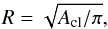 (8)where Acl is the clump
projected area in the sky; FWHM is the clump full width at half maximum computed
as
(8)where Acl is the clump
projected area in the sky; FWHM is the clump full width at half maximum computed
as 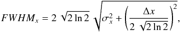 (9)where x ∈ {
l,b,v }. The second
term under the big square root represents the pixel resolution term and ensures that the
FWHM is not
smaller than the pixel size. For the GRS data cube, the pixel size Δx is
(9)where x ∈ {
l,b,v }. The second
term under the big square root represents the pixel resolution term and ensures that the
FWHM is not
smaller than the pixel size. For the GRS data cube, the pixel size Δx is
 , which corresponds at
N107’s distance of 3600 pc to
0.39 pc × 0.39 pc × 0.21 km
s-1. If Δx goes to zero, the FWHM approaches the Gaussian
FWHM.
, which corresponds at
N107’s distance of 3600 pc to
0.39 pc × 0.39 pc × 0.21 km
s-1. If Δx goes to zero, the FWHM approaches the Gaussian
FWHM.
The value of  is the variance
weighted by the brightness temperature Tb,
is the variance
weighted by the brightness temperature Tb,
 with
the summation taken over all pixels belonging to the clump. The variable M is the clump mass, which is
the total mass of pixels belonging to the clump, derived from Eqs. (3)–(6) (Sect. 2.4). The error of the clump mass,
assuming Gaussian noise and neglecting pixel correlation within the beam, is
with
the summation taken over all pixels belonging to the clump. The variable M is the clump mass, which is
the total mass of pixels belonging to the clump, derived from Eqs. (3)–(6) (Sect. 2.4). The error of the clump mass,
assuming Gaussian noise and neglecting pixel correlation within the beam, is
 (12)where Npx is the number
of pixels of the clump and ΔMpx is the σnoise equivalent
mass; in our case of the GRS 13CO data cubes, σnoise = 0.34 K ⇒
ΔMpx = 0.21 M⊙;
Mvir is the clump virial mass, estimated as
(MacLaren et al. 1988):
(12)where Npx is the number
of pixels of the clump and ΔMpx is the σnoise equivalent
mass; in our case of the GRS 13CO data cubes, σnoise = 0.34 K ⇒
ΔMpx = 0.21 M⊙;
Mvir is the clump virial mass, estimated as
(MacLaren et al. 1988):  (13)The formula above
assumes a spherical clump with a density profile ∝1
/r; ΔMvir is the
virial mass error derived from the first order Taylor expansion of Eq. (13), assuming the clump’s area and
FWHMv
errors of one pixel.
(13)The formula above
assumes a spherical clump with a density profile ∝1
/r; ΔMvir is the
virial mass error derived from the first order Taylor expansion of Eq. (13), assuming the clump’s area and
FWHMv
errors of one pixel.
Figure 8 shows a histogram of clumps masses. Overlaid is a line representing a fit by a function dN/ dM = C(M/M⊙)α, where α is the slope of the clump mass function and C is a constant. We used least-squares fitting on a logarithmic scale, i.e. we fit the log of the bin heights log (dN/ dM) by a function log (C(M/M⊙)α). The best fitting slope is α = − 1.1. The bins in the histogram have variable widths, set so that each contains seven clumps. This ensures that all bins have the same significance.
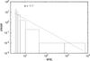 |
Fig. 8 Histogram of the mass spectrum of molecular clumps associated with bubble N107. The bin widths are variable, set so that each bin contains seven clumps. The dashed line represents the best fitting power-law function with the index α = −1.1. |
4. Numerical simulations of bubbles and comparison with N107
We simulated the evolution of bubbles formed in the ISM around massive stars in order to estimate parameters of N107 that cannot be derived directly from observation (especially its age). We used a version of the FORTRAN code ring (Palouš 1990; Ehlerová & Palouš 1996), which was originally written for simulations of expanding H i shells in the Galactic ISM.
4.1. Code description
The simulation starts with a small spherical shell, which is set according to the
wind-blown bubble model of Weaver et al. (1977) in
the pressure-driven snowplough phase. The infinitesimally thin shell (thin-shell
approximation) is divided into nl×np elements. We solve the equations of motion
including the pressure difference between the shell interior and exterior and the mass
accumulation of the ambient medium. We do not include gravity or any other force acting on
the shell. The momentum equation for an element is  (14)where m is the element mass,
v is the element velocity,
S is the element surface, and
Pi and Pe are the
interior and exterior pressures. The total number of elements is fixed (we used
30 × 60), so their surface
and mass grow with time. The mass growth is given by the equation
(14)where m is the element mass,
v is the element velocity,
S is the element surface, and
Pi and Pe are the
interior and exterior pressures. The total number of elements is fixed (we used
30 × 60), so their surface
and mass grow with time. The mass growth is given by the equation  (15)where ρ is the local density of
the ambient medium.
(15)where ρ is the local density of
the ambient medium.
For the sake of simplicity, an energy source is represented as a continuous and constant
energy input Ė. For each timestep a corresponding amount of energy
is added to the bubble interior and a new value of the interior pressure is computed as
 (16)where
Ei is the interior thermal energy and
V is the
bubble volume. Equation (16) assumes that
the interior is filled with monoatomic gas expanding adiabatically. In the case of a shell
expanding into a uniform medium, this type of energy source gives for the shell radius, as
a function of time, a power law with an index 3
/ 5. This is between the power-law index
2 / 5,
given by a single (supernova) explosion and the power-law index 4 / 7, valid for an
expanding H ii region.
(16)where
Ei is the interior thermal energy and
V is the
bubble volume. Equation (16) assumes that
the interior is filled with monoatomic gas expanding adiabatically. In the case of a shell
expanding into a uniform medium, this type of energy source gives for the shell radius, as
a function of time, a power law with an index 3
/ 5. This is between the power-law index
2 / 5,
given by a single (supernova) explosion and the power-law index 4 / 7, valid for an
expanding H ii region.
The motion of the bubble elements is integrated using the fourth-order Runge-Kutta method with adaptive timestep.
4.2. Simulation setup
We assume a bubble expanding in a molecular cloud with a 3D Gaussian density profile (see
Fig. 9), ![Mathematical equation: \begin{equation} \label{eq_ring_density_profile} n = n_0 \exp \left\{ -\frac{1}{2} \left[ \left(\frac{x-x_0}{\sigma_x}\right)^2 + \left(\frac{y-y_0}{\sigma_y}\right)^2 + \left(\frac{z-z_0}{\sigma_z}\right)^2 \right] \right\}, \end{equation}](/articles/aa/full_html/2014/05/aa22687-13/aa22687-13-eq221.png) (17)
(17)
where n is the particle density; n0 is the particle density in the centre of the cloud; σx, σy, σz are the Gaussian thicknesses (standard deviation) in the x, y, z direction; x0, y0, z0 specify the location of the cloud centre.
We also assume the centre of expansion is shifted/dislocated from the centre of the cloud
by Δr0 towards direction (−x, −y). In the code, the
expansion centre (bubble centre) is located at x = y = z = 0, so
we shift the cloud centre by Δr0 in the xy plane: 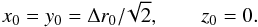 (18)We assume a hydrogen
abundance of X =
0.735, helium abundance of Y = 0.245, metallicity of Z = 0.02, and a mean
relative particle weight of metals of 16.65. We also assume that all hydrogen in the cloud is in the form of
H2. This yields a
mean relative particle weight of the molecular matter of μ = 2.34. The molecular
material of the cloud is isothermal with the temperature set at 20 K. We also consider the atomic gas
component, which is represented by a density background with the constant value of
4 hydrogen atoms per
cm3 and a
temperature of 6000 K. The
total initial energy of the bubble is set to 1
× 1049 erg and each time step δt the energy is increased
by Ėδt.
(18)We assume a hydrogen
abundance of X =
0.735, helium abundance of Y = 0.245, metallicity of Z = 0.02, and a mean
relative particle weight of metals of 16.65. We also assume that all hydrogen in the cloud is in the form of
H2. This yields a
mean relative particle weight of the molecular matter of μ = 2.34. The molecular
material of the cloud is isothermal with the temperature set at 20 K. We also consider the atomic gas
component, which is represented by a density background with the constant value of
4 hydrogen atoms per
cm3 and a
temperature of 6000 K. The
total initial energy of the bubble is set to 1
× 1049 erg and each time step δt the energy is increased
by Ėδt.
 |
Fig. 9 Simulation setup for a stellar-blown bubble. The bubble is formed around one or more massive stars inside a molecular cloud, with a 3D Gaussian density profile. The Gaussian thickness σx and σy in the sky plane is set to 12 pc, while σz, which runs parallel to our LOS, is a parameter we vary. The centre of expansion is dislocated from the centre of the cloud by Δr0, which is another parameter we vary. The dislocation is towards the (−x, − y) direction, perpendicular to the LOS. The molecular cloud is overlaid on a background of atomic gas with the particle density of 4 cm-3. |
4.3. Comparison with observation
We ran a series of simulations in order to find the parameters that produce a bubble with similar mass distribution and expansion velocity to N107. The varying input parameters for ring were the energy input (Ė), the shift/dislocation of the expansion centre from the cloud centre (Δr0), the Gaussian thickness of the cloud in the direction of our line of sight (LOS) (σz), and the total mass of the molecular cloud (M0). The Gaussian thickness in the sky plane σxy = σx = σy was kept constant at 12 pc, which is comparable to the radius of N107. For each set of these parameters, the code evolves a bubble in time and outputs a chain of its snapshots in given time intervals.
Because the bubble is expanding in an inhomogeneous, non-spherical density field, the elements facing a lower density expand faster. This causes the bubble’s geometrical centre to move progressively towards the direction of a lower density. To compensate for this drift, we centred each snapshot at the bubble’s geometrical centre, which is computed as the mean (x,y,z) coordinates of the bubble elements weighted by their surfaces. We projected these centred snapshots onto FITS data cubes with two spatial (XY) and one radial velocity (RV) dimensions with the same pixel size as in the GRS data cube.
The radiation from OB stars illuminating molecular clouds creates a layer of dissociated matter. This layer then serves as a shield against the radiation and prevents it from penetrating farther inside. The dissociated matter will not contribute to the 13CO line brightness temperature. To account for that, before computing the 13CO line brightness temperature, we decreased the surface density of each bubble element by 4.35 M⊙ pc-2. This value is based on the suggestion for shielding by Krumholz et al. (2009). We assume that the 13CO abundances are the same as we used for measuring the observed molecular mass in Sect. 2.4. Then for each pixel we derived the corresponding brightness temperature of the 13CO (J = 1−0) line. Finally, we applied convolution to simulate the FCRAO telescope resolution used in the GRS. The resulting FITS thus represents an image, which would be seen by FCRAO if it observed the simulated bubble at a given evolution time.
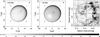 |
Fig. 10 Snapshots from the best fitting simulations from group A (left) and B (centre) and GRS observation (right). Shown is the brightness temperature of the 13CO line integrated over the radial velocities of ± 8 km s-1 relative to the radial velocity of the bubble centre. The images also show four sectors used to compare the angular mass distribution (see Sect. 4.3 and Eq. (21)). The plus sign (+) in pictures A and B marks the original expansion centre. Aperture 2, shown in the GRS picture, marks which region from the observed data we used for comparison with simulations. |
We define a goodness-of-fit parameter δ, to compare the synthetic data cubes to the
observations: ![Mathematical equation: \begin{equation} \label{eq_delta} \delta = \frac{1}{3}\left[ \delta V_\mathrm{exp}^2 + \frac{1}{4}\sum_{i\,=\,1}^{4}\left( \delta m_i^2 + \delta r_i^2 \right) \right]. \end{equation}](/articles/aa/full_html/2014/05/aa22687-13/aa22687-13-eq259.png) (19)Lower values of
δ mean a
better fit to (better agreement with) the observed properties of N107. The meaning of the
terms is as follows:
(19)Lower values of
δ mean a
better fit to (better agreement with) the observed properties of N107. The meaning of the
terms is as follows:  (20)represents
the square of the difference of the bubble expansion velocity between the observed value
of N107 (Vexp, o) and
simulated value (Vexp, s). We adopt
the observed bubble expansion velocity of Vexp, o = 8 km
s-1, which is derived from the H i observations and
represents half of the relative velocity of the shell’s front and back wall;
(20)represents
the square of the difference of the bubble expansion velocity between the observed value
of N107 (Vexp, o) and
simulated value (Vexp, s). We adopt
the observed bubble expansion velocity of Vexp, o = 8 km
s-1, which is derived from the H i observations and
represents half of the relative velocity of the shell’s front and back wall; ![Mathematical equation: \begin{equation} \label{eq_circular_sectors_sum} \frac{1}{4}\sum_{i\,=\,1}^{4}\left( \delta m_i^2 + \delta r_i^2 \right) = \frac{1}{4}\sum_{i\,=\,1}^{4}\left( \left[ \frac{m_{i,\,\mathrm{s}} - m_{i,\,\mathrm{o}}}{m_{i,\,\mathrm{o}}} \right]^2 +\left[ \frac{r_{i,\,\mathrm{s}} - r_{i,\,\mathrm{o}}}{r_{i,\,\mathrm{o}}} \right]^2 \right) \end{equation}](/articles/aa/full_html/2014/05/aa22687-13/aa22687-13-eq264.png) (21)
(21)
is a sum taken over four circular sectors of aperture 2 used to measure the bubble
molecular mass (see Sect. 2.4). This term compares
the angular mass distribution between N107 and the simulated bubbles. A visualisation of
the sectors is shown in Fig. 10. The values
mi,
s and mi, o are the simulated
(“s”) and observed (“o”) molecular masses in circular sector i; ri,
s and ri, o give the
simulated and observed mean radii in sector i, weighted by the brightness temperature
 (22)where the sums are taken
over the pixels in sector i.
(22)where the sums are taken
over the pixels in sector i.
Ranges of the input parameters Ė, r0, σz, M0; and the constraint of the evolution time (t) used for the numerical simulations of expanding bubbles.
First, we ran a series of simulations with a wider span of the input parameters Ė, r0, σz, and M0 with steps on a logarithmic scale and the evolution time up to t = 100 Myr with snapshots taken every 0.5 Myr. Then we located a subset of the input parameters with best fits to the observation (lowest δ) and ran a second series of simulations with finer parameter resolutions. In the second series, we used linear steps for parameters r0 and σz and logarithmic steps for Ė and M0. The snapshots were taken every 0.25 Myr up to t = 8 Myr. We note that the internal time step of ring is controlled dynamically by its Runge-Kutta routines; we only set the snapshot printout interval Δt. Parameters for both runs are listed in Table 3. The ten best fitting runs are shown in Table 4.
First ten sets of parameters best fitting the observation of N107.
To conclude, we simulated the evolution of bubbles formed around massive stars in molecular clouds and compared their properties to N107. We got the best agreement for two groups of parameters:
-
1.
Group A represents bubbles pro-duced with a lower energy input(Ė< 0.4 × 1050 erg / Myr), greater centre-of-expansion dislocation (r0 ≈ 16...22 pc), formed within an oblate molecular cloud with the oblateness of (σz/σxy = 6 / 12), and with a greater evolution time (t ≈ 1.75...2.25 Myr).
-
2.
Group B represents bubbles produced with a higher energy input (Ė = 2.7 × 1050 erg / Myr), smaller centre-of-expansion dislocation (r0 ≈ 10...12 pc), formed within a prolate molecular cloud (σz/σxy ≈ (20...28) / 12), with a smaller evolution time (t = 1 Myr).
Fits show little sensitivity to the parameter M0, the initial mass of the surrounding
molecular cloud (M0
≈ 5.8...15.5 ×
105 M⊙). Both groups of the
best-fitting-simulations suggest that bubble N107 is relatively young
( ) and was formed at the very edge
of its parental molecular cloud.
) and was formed at the very edge
of its parental molecular cloud.
Figure 10 shows snapshots from the best fitting simulations from both groups A and B and the GRS observation of the CO line.
5. Discussion
5.1. Numerical simulation setup, assumptions, and validity of approximations
An important assumption for the simulation setup is the shape and density profile of the parental molecular cloud. In our simulations, we chose the Gaussian density profile and tested different levels of the oblateness (ratio of σz to σxy). The oblate shape of the parental molecular clouds that host bubbles similar to N107 is supported by a study of Beaumont & Williams (2010), who concluded that the Spitzer bubbles are formed in oblate, sheet-like, molecular clouds with a thickness of a few parsecs. Our simulations, however, favour neither oblate nor prolate clouds.
The numerical code ring assumes the thin-shell approximation, which is applicable so long as the bubble expansion is supersonic, i.e. expanding with a velocity higher than the sound speed of the ambient cold gas: ≈0.3 km s-1 (for T = 20 K, γ = 7 / 5, μ = 2.34). In our runs, almost all the bubble’s elements move faster through the ambient gas during the whole bubble evolution, so the thin-shell approximation is reasonable. Moreover, if the speed of an element decreases below the sound speed, the code stops the mass accumulation for that element.
5.2. Source of radio continuum
The radio continuum emission coming from the direction of the bubble interior has both thermal and nonthermal components. While the strong radio source A is dominated by nonthermal radiation, the fainter source B is emitting thermally (Fig. 6). The nonthermal source A is brighter than the thermal source B by almost one order of magnitude, so we can expect that the thermal emission is present in the whole bubble volume, only outshone in aperture A by the nonthermal source. The mixing of thermal and nonthermal radiation in aperture A is also suggested by the visual comparison of the radio continuum and the 24 μm emission (Fig. 7). The northern part of aperture A features both the radio continuum and the 24 μm emission, while in the southern part only the radio continuum is observed. Furthermore, the merging of thermal and nonthermal radiation in aperture A explains why the measured spectral index (−0.3) is closer to 0 than the typical value for supernova remnants (−0.5, the average value in the supernova remnants catalogue of Green 2009).
The negative spectral indices of sources C (−0.2) and D (−0.1) suggest that part of their radio continuum is also emitted by a nonthermal source. The nonthermal contribution to the flux is stronger for source C than for source D. This is expected, since aperture D covers a distinct 24 μm (thermal) source, while there is almost no 24 μm emission in aperture C (Fig. 7).
Given that first supernovae in an OB association explode only after 3 Myr or later, and considering the bubble evolution time estimated from simulations (<2.25 Myr), no supernova remnant should be present inside the bubble yet. In other words, our analysis suggests that a supernova remnant not associated with the bubble may be present in the direction towards the bubble.
5.3. Missing OB association
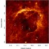 |
Fig. 11 Possible stellar progenitors (white plus signs) of bubble N107 found in the UKIDSS catalogue. The numerical labels of the stars correspond to the labels in Table 5. The background is the 8 μm emission taken from GLIMPSE. |
Possible stellar progenitors of bubble N107 found in the UKIDSS catalogue.
We searched the SIMBAD database and a catalogue of Galactic OB stars by Reed (2003) for sources which could be responsible for the bubble creation. However, no OB star, supernova remnant, or pulsar is known to lie in the direction of the bubble interior or in its vicinity.
We also performed a search for massive stars possibly related to N107 using the UKIDSS catalogue 7th data release (Lawrence et al. 2007), stellar evolutionary tracks by Bressan et al. (2012), and the standard model of extinction (Rieke & Lebofsky 1985). We derived the extinction for the massive star candidates in the field of N107 and compared it to the values of extinction given for that direction by Stead & Hoare (2009). The search for massive stars involves many uncertainties, but the comparison of the derived extinctions with independent values is a good test of the credibility of our results. We ended up with six massive star candidates, which lie at distances comparable with the distance of N107 (3.6 kpc). None of these six stars has measured radial velocities. Three of them lie at the rim of the bubble, so they can hardly be its progenitors, but the others are possible energy sources. The selected massive stars are shown in Fig. 11 and are listed in Table 5.
5.4. Molecular clump mass spectrum
The best fitting slope for the mass spectrum of molecular clumps found along the borders of N107 is −1.1 (Fig. 8). This is a significantly shallower slope than that of the classical stellar initial mass function (Salpeter: −2.35) and also shallower than the clump mass function slope from −1.6 to −1.8 derived by Kramer et al. (1998). We note that Kramer et al. (1998) used Gaussian decomposition for clump identification, which is a fundamentally different method than we used and, moreover, studied different types of clouds, not shell-like as is the case for N107.
The least massive clumps we found have masses of about 3.5 M⊙. This limit is given by the angular resolution and sensitivity of the observations of the 13CO line. With better resolution and sensitivity, we expect that some clumps, especially the most massive ones, would be identified as several less massive clumps. This would alter the shape of the clump mass spectrum, and very likely redistribute the mass of the largest clumps into less massive ones, so that the slope would be steeper.
6. Conclusion
We studied dust bubble N107, discovered by Churchwell et al. (2006) with infrared observations by the Spitzer Space Telescope. Radio observations of the H i and 13CO (J = 1−0) lines revealed its atomic and molecular components, which allowed us to determine the bubble’s radial velocity, kinematical distance, and the mass of these components. Using the code DENDROFIND (Wünsch et al. 2012) we decomposed the molecular ring associated with the bubble into 49 individual clumps and found that the clump mass spectrum slope is about − 1.1. Radio continuum observations at 1420 MHz and 327 MHz suggest the radio flux coming from the bubble direction has both thermal and nonthermal components; i.e. besides a classical H ii region, a supernova remnant contributes to the emission. We simulated the evolution of stellar-blown bubbles within molecular clouds with the numerical code ring (Palouš 1990; Ehlerová & Palouš 1996). We were able to produce two groups of bubbles with a similar angular mass distribution and expansion velocity to N107: (A) bubbles formed within an oblate molecular cloud (σz/σxy = 6 / 12), with the energy input Ė< 0.4 × 1050 erg / Myr and the evolution time t ≈ 1.75...2.25 Myr, and (B) bubbles formed within a prolate molecular cloud (σz/σxy = (20...28) / 12), with the energy input Ė ≈ 2.7 × 1050 erg / Myr and the evolution time t = 1 Myr. Considering the estimated bubble evolution time (<2.25 Myr), no supernova remnant should be present inside the bubble, yet. This may be explained by a supernova remnant present in the direction towards the bubble, but not associated with it. A summary of the parameters we derived for bubble N107, together with the parameters given by Churchwell et al. (2006), is presented in Table 6.
Summary of parameters derived for N107.
LSR = local standard of rest.
FWHM = Full width at half maximum.
FITS = Flexible Image Transport System (Pence et al. 2010).
Acknowledgments
We thank the anonymous referee for multiple constructive suggestions which led to improvements of the paper. This work was supported by the project RVO: 67985815. VS acknowledges support from a Marie Curie fellowship as part of the European Commission FP6 Research Training Network “Constellation” under contract MCRTN–CT–2006-035890; support from Doctoral grant of the Czech Science Foundation No. 205/09/H033. R.W. acknowledges support from the project P209/12/1795 of the Czech Science Foundation. The research leading to these results has received funding from the European Community’s Seventh Framework Programme under grant agreement no. PIIF-GA-2008-221289. This research has made use of SAOImage DS9, developed by Smithsonian Astrophysical Observatory (Joye & Mandel 2003). This research has made use of the SIMBAD database, operated at CDS, Strasbourg, France. This research has made use of NASA’s Astrophysics Data System. This research has made use of the NASA/IPAC Infrared Science Archive, which is operated by the Jet Propulsion Laboratory, California Institute of Technology, under contract with the National Aeronautics and Space Administration. This publication has made use of molecular line data from the Boston University-FCRAO Galactic Ring Survey (GRS). The GRS is a joint project of Boston University and Five College Radio Astronomy Observatory, funded by the National Science Foundation under grants AST-9800334, AST-0098562, & AST-0100793.
References
- Beaumont, C. N., & Williams, J. P. 2010, ApJ, 709, 791 [NASA ADS] [CrossRef] [Google Scholar]
- Benjamin, R. A., Churchwell, E., Babler, B. L., et al. 2003, PASP, 115, 953 [NASA ADS] [CrossRef] [Google Scholar]
- Binney, J., & Merrifield, M. 1998, Galactic Astronomy (Princeton: Princeton University Press) [Google Scholar]
- Brand, J., & Blitz, L. 1993, A&A, 275, 67 [NASA ADS] [Google Scholar]
- Bressan, A., Marigo, P., Girardi, L., et al. 2012, MNRAS, 427, 127 [NASA ADS] [CrossRef] [Google Scholar]
- Carey, S. J., Noriega-Crespo, A., Mizuno, D. R., et al. 2009, PASP, 121, 76 [NASA ADS] [CrossRef] [Google Scholar]
- Casali, M., Adamson, A., Alves de Oliveira, C., et al. 2007, A&A, 467, 777 [NASA ADS] [CrossRef] [EDP Sciences] [Google Scholar]
- Castor, J., McCray, R., & Weaver, R. 1975, ApJ, 200, L107 [NASA ADS] [CrossRef] [Google Scholar]
- Chevalier, R. A. 1974, ApJ, 188, 501 [NASA ADS] [CrossRef] [Google Scholar]
- Churchwell, E., Povich, M. S., Allen, D., et al. 2006, ApJ, 649, 759 [NASA ADS] [CrossRef] [Google Scholar]
- Condon, J. J., & Ransom, S. M. 2010, Essential Radio Astronomy (National Radio Astronomy Observatory), (online; http://www.cv.nrao.edu/course/astr534/ERA.shtml) [Google Scholar]
- Deharveng, L., Schuller, F., Anderson, L. D., et al. 2010, A&A, 523, A6 [NASA ADS] [CrossRef] [EDP Sciences] [Google Scholar]
- Dib, S., & Burkert, A. 2005, ApJ, 630, 238 [NASA ADS] [CrossRef] [Google Scholar]
- Draine, B. T. 2003, ARA&A, 41, 241 [NASA ADS] [CrossRef] [Google Scholar]
- Duvert, G., Cernicharo, J., Bachiller, R., & Gomez-Gonzalez, J. 1990, A&A, 233, 190 [NASA ADS] [Google Scholar]
- Efremov, Y. N., Elmegreen, B. G., & Hodge, P. W. 1998, ApJ, 501, L163 [NASA ADS] [CrossRef] [Google Scholar]
- Efremov, Y. N., Ehlerová, S., & Palouš, J. 1999, A&A, 350, 457 [NASA ADS] [Google Scholar]
- Ehlerová, S., & Palouš, J. 1996, A&A, 313, 478 [NASA ADS] [Google Scholar]
- Ehlerová, S., & Palouš, J. 2005, A&A, 437, 101 [NASA ADS] [CrossRef] [EDP Sciences] [Google Scholar]
- Elmegreen, B. G. 1994, ApJ, 427, 384 [NASA ADS] [CrossRef] [Google Scholar]
- Elmegreen, B. G., & Lada, C. J. 1977, ApJ, 214, 725 [NASA ADS] [CrossRef] [Google Scholar]
- Green, D. A. 2009, VizieR Online Data Catalog: VII/253 [Google Scholar]
- Hambly, N. C., Collins, R. S., Cross, N. J. G., et al. 2008, MNRAS, 384, 637 [NASA ADS] [CrossRef] [Google Scholar]
- Heiles, C. 1979, ApJ, 229, 533 [NASA ADS] [CrossRef] [Google Scholar]
- Heiles, C. 1984, ApJS, 55, 585 [NASA ADS] [CrossRef] [Google Scholar]
- Hewett, P. C., Warren, S. J., Leggett, S. K., & Hodgkin, S. T. 2006, MNRAS, 367, 454 [NASA ADS] [CrossRef] [Google Scholar]
- Irwin, M. J., Lewis, J., Hodgkin, S., et al. 2004, in Optimizing Scientific Return for Astronomy through Information Technologies, eds. P. J. Quinn, & A. Bridger, SPIE Conf. Ser., 5493, 411 [Google Scholar]
- Jackson, J. M., Rathborne, J. M., Shah, R. Y., et al. 2006, ApJS, 163, 145 [NASA ADS] [CrossRef] [Google Scholar]
- Joye, W. A., & Mandel, E. 2003, in Astronomical Data Analysis Software and Systems XII, eds. H. E. Payne, R. I. Jedrzejewski, & R. N. Hook, ASP Conf. Ser., 295, 489 [Google Scholar]
- Kahn, F. D. 1954, Bull. Astron. Inst. Netherlands, 12, 187 [NASA ADS] [Google Scholar]
- Kellermann, K. I., & Verschuur, G. L. 1988, Galactic and extragalactic radio astronomy, 2nd edn. (Berlin, New York: Springer Verlag) [Google Scholar]
- Kiss, C., Moór, A., & Tóth, L. V. 2004, A&A, 418, 131 [NASA ADS] [CrossRef] [EDP Sciences] [Google Scholar]
- Könyves, V., Kiss, C., Moór, A., Kiss, Z. T., & Tóth, L. V. 2007, A&A, 463, 1227 [NASA ADS] [CrossRef] [EDP Sciences] [Google Scholar]
- Koo, B.-C., Gibson, S. J., Kang, J.-H., et al. 2010, Highlights of Astronomy, 15, 788 [NASA ADS] [Google Scholar]
- Kramer, C., Stutzki, J., Rohrig, R., & Corneliussen, U. 1998, A&A, 329, 249 [NASA ADS] [Google Scholar]
- Krumholz, M. R., McKee, C. F., & Tumlinson, J. 2009, ApJ, 693, 216 [NASA ADS] [CrossRef] [Google Scholar]
- Lawrence, A., Warren, S. J., Almaini, O., et al. 2007, MNRAS, 379, 1599 [NASA ADS] [CrossRef] [MathSciNet] [Google Scholar]
- Lefloch, B., & Lazareff, B. 1994, A&A, 289, 559 [NASA ADS] [Google Scholar]
- Loeb, A., & Perna, R. 1998, ApJ, 503, L35 [NASA ADS] [CrossRef] [Google Scholar]
- MacLaren, I., Richardson, K. M., & Wolfendale, A. W. 1988, ApJ, 333, 821 [NASA ADS] [CrossRef] [Google Scholar]
- Oort, J. H., & Spitzer, Jr., L. 1955, ApJ, 121, 6 [NASA ADS] [CrossRef] [Google Scholar]
- Paladini, R., Burigana, C., Davies, R. D., et al. 2003, A&A, 397, 213 [NASA ADS] [CrossRef] [EDP Sciences] [Google Scholar]
- Palouš, J. 1990, in IAU Symp., 144, 101P [Google Scholar]
- Pavlyuchenkov, Y. N., Kirsanova, M. S., & Wiebe, D. S. 2013, Astron. Rep., 57, 573 [NASA ADS] [CrossRef] [Google Scholar]
- Peek, J. E. G., Heiles, C., Douglas, K. A., et al. 2011, ApJS, 194, 20 [NASA ADS] [CrossRef] [Google Scholar]
- Pence, W. D., Chiappetti, L., Page, C. G., Shaw, R. A., & Stobie, E. 2010, A&A, 524, A42 [NASA ADS] [CrossRef] [EDP Sciences] [Google Scholar]
- Reach, W. T., Rho, J., Tappe, A., et al. 2006, AJ, 131, 1479 [NASA ADS] [CrossRef] [Google Scholar]
- Reed, B. C. 2003, AJ, 125, 2531 [NASA ADS] [CrossRef] [Google Scholar]
- Rieke, G. H., & Lebofsky, M. J. 1985, ApJ, 288, 618 [NASA ADS] [CrossRef] [Google Scholar]
- Rohlfs, K., & Wilson, T. L. 1996, Tools of Radio Astronomy Astron. Astrophys. Lib (Heidelberg, Berlin, New York: Springer Verlag) [Google Scholar]
- Rosolowsky, E. W., Pineda, J. E., Kauffmann, J., & Goodman, A. A. 2008, ApJ, 679, 1338 [NASA ADS] [CrossRef] [Google Scholar]
- Simpson, R. J., Povich, M. S., Kendrew, S., et al. 2012, MNRAS, 424, 2442 [NASA ADS] [CrossRef] [Google Scholar]
- Sonnentrucker, P., Welty, D. E., Thorburn, J. A., & York, D. G. 2007, ApJS, 168, 58 [NASA ADS] [CrossRef] [Google Scholar]
- Spitzer, L. 1978, Physical processes in the interstellar medium (New York: Wiley-Interscience) [Google Scholar]
- Stead, J. J., & Hoare, M. G. 2009, MNRAS, 400, 731 [NASA ADS] [CrossRef] [Google Scholar]
- Stil, J. M., Taylor, A. R., Dickey, J. M., et al. 2006, AJ, 132, 1158 [NASA ADS] [CrossRef] [Google Scholar]
- Taylor, A. R., Goss, W. M., Coleman, P. H., van Leeuwen, J., & Wallace, B. J. 1996, ApJS, 107, 239 [NASA ADS] [CrossRef] [Google Scholar]
- Tenorio-Tagle, G., & Bodenheimer, P. 1988, ARA&A, 26, 145 [NASA ADS] [CrossRef] [Google Scholar]
- Visser, R., van Dishoeck, E. F., & Black, J. H. 2009, A&A, 503, 323 [NASA ADS] [CrossRef] [EDP Sciences] [Google Scholar]
- Weaver, R., McCray, R., Castor, J., Shapiro, P., & Moore, R. 1977, ApJ, 218, 377 [NASA ADS] [CrossRef] [Google Scholar]
- Whitworth, A. P., Bhattal, A. S., Chapman, S. J., Disney, M. J., & Turner, J. A. 1994, MNRAS, 268, 291 [NASA ADS] [CrossRef] [Google Scholar]
- Wilson, T. L. 1999, Rep. Prog. Phys., 62, 143 [Google Scholar]
- Wünsch, R., Jáchym, P., Sidorin, V., et al. 2012, A&A, 539, A116 [NASA ADS] [CrossRef] [EDP Sciences] [Google Scholar]
All Tables
Radio continuum flux densities and spectral indices for apertures A, B, C, and D.
Ranges of the input parameters Ė, r0, σz, M0; and the constraint of the evolution time (t) used for the numerical simulations of expanding bubbles.
All Figures
|
Fig. 1 Bubble N107 – false colour multiwavelength image. The 24 μm continuum (red) is dominated by the emission of very small dust grains heated by a nearby massive star. The 8 μm continuum (green) is dominated by the emission of PAHs, large molecules found within molecular clouds. The CO line (blue) is integrated over the radial velocities between 38.5 km s-1 and 47.6 km s-1 and traces the cold gas of molecular clouds. The distinct red-green structure seen in the lower-left in the direction of the bubble’s opening is probably not related to the bubble, since the radial velocity of the associated molecular material (≈60 km s-1) differs significantly from the radial velocity of the N107 complex (≈43 km s-1). |
| In the text | |
|
Fig. 2 Brightness temperature maps of the H i line in several velocity channels. An outline of bubble N107 as given in the catalogue of Churchwell et al. (2006) is marked with the dashed grey circle. The channels 41.0 km s-1 and 41.9 km s-1 show morphology very similar to that of the 8 μm emission. |
| In the text | |
|
Fig. 3 Brightness temperature of the H i line in an l −
v diagram: a cut through
|
| In the text | |
|
Fig. 4 Apertures for measuring the mass associated with bubble N107. The pixels lying within the apertures contribute to the measured masses. The dashed circles mark bubble N107 as was identified in the 8 μm emission by Churchwell et al. (2006). Left: H i line emission at 42.8 km s-1. The innermost circle (BG) is the region we used to derive the background emission. Right: 13CO line emission at 42.8 km s-1. We used two apertures to measure the molecular mass. Aperture 1 is the same as that for measuring the H i mass, while aperture 2 is smaller and covers only the immediate vicinity of the bubble. |
| In the text | |
|
Fig. 5 Brightness temperature maps of the 13CO (J = 1 − 0) emission in several velocity channels in degrees Kelvin. An outline of bubble N107 as given in the catalogue of Churchwell et al. (2006) is marked with the dashed grey circle. |
| In the text | |
|
Fig. 6 Radio continuum emission associated with bubble N107. The bubble is denoted by the grey dashed circle in the centre. Overlaid are four elliptical apertures (A, B, C, D) used to measure the radio fluxes. The grey dashed ellipse in the upper right (labelled BG) is the region used for measuring the background. Left: emission at 1420 MHz/21 cm from the VGPS survey. Right: emission at 327 MHz/92 cm from the WSRT survey. We note blurring in the direction of declination (top-left-to-bottom-right), caused by the larger beam size (lower resolution) in the declination direction. |
| In the text | |
|
Fig. 7 Comparison of the VGPS radio continuum at 1420 MHz/21 cm (blue) with the 8 μm (green) and 24 μm (red) emission. Left: 1420 MHz and 8 μm emission. The radio continuum follows the bubble outline and fills part of its interior. Right: same as left with added 24 μm emission. Inside the bubble, the radio continuum is well correlated with the 24 μm emission, except for the eastern part, where the 24 μm emission is absent and only the radio continuum is observed. |
| In the text | |
|
Fig. 8 Histogram of the mass spectrum of molecular clumps associated with bubble N107. The bin widths are variable, set so that each bin contains seven clumps. The dashed line represents the best fitting power-law function with the index α = −1.1. |
| In the text | |
|
Fig. 9 Simulation setup for a stellar-blown bubble. The bubble is formed around one or more massive stars inside a molecular cloud, with a 3D Gaussian density profile. The Gaussian thickness σx and σy in the sky plane is set to 12 pc, while σz, which runs parallel to our LOS, is a parameter we vary. The centre of expansion is dislocated from the centre of the cloud by Δr0, which is another parameter we vary. The dislocation is towards the (−x, − y) direction, perpendicular to the LOS. The molecular cloud is overlaid on a background of atomic gas with the particle density of 4 cm-3. |
| In the text | |
|
Fig. 10 Snapshots from the best fitting simulations from group A (left) and B (centre) and GRS observation (right). Shown is the brightness temperature of the 13CO line integrated over the radial velocities of ± 8 km s-1 relative to the radial velocity of the bubble centre. The images also show four sectors used to compare the angular mass distribution (see Sect. 4.3 and Eq. (21)). The plus sign (+) in pictures A and B marks the original expansion centre. Aperture 2, shown in the GRS picture, marks which region from the observed data we used for comparison with simulations. |
| In the text | |
|
Fig. 11 Possible stellar progenitors (white plus signs) of bubble N107 found in the UKIDSS catalogue. The numerical labels of the stars correspond to the labels in Table 5. The background is the 8 μm emission taken from GLIMPSE. |
| In the text | |
Current usage metrics show cumulative count of Article Views (full-text article views including HTML views, PDF and ePub downloads, according to the available data) and Abstracts Views on Vision4Press platform.
Data correspond to usage on the plateform after 2015. The current usage metrics is available 48-96 hours after online publication and is updated daily on week days.
Initial download of the metrics may take a while.