© ESO, 2014

1. Introduction

1.1. Context and scope

Stellar interferometers deliver data that are related to the Fourier transform (FT) of the intensity distribution perpendicular to the line of sight. Ideally, these interferometers are able to measure complex visibilities, which correspond to complex samples of this FT at spatial frequencies defined by the positions of the interfering either telescopes or antennas and by the observation wavelength λ. In essence, measuring moduli and phases of complex visibilities amounts to measuring contrasts and phases of interference fringes (Cornwell 1987; Labeyrie 1975).

In contrast to radio interferometric arrays, however, current optical interferometers cannot measure the phases of the complex Fourier samples because of rapid (10 to 20 ms) perturbations caused by atmospheric turbulence. Instead, they provide both their moduli (the so-called absolute visibilities) or their squared values (the power spectrum) by measuring contrasts in snapshot mode with short integration times that freeze the turbulence and determine a linear relationships between their phase (the phase closure) (Roddier & Lena 1984; Roddier 1986; Mourard et al. 1994).

The (squared) visibility moduli are without a doubt the instrumental interferometric data that is the most used by the astronomical community. It is generally assumed that the distribution of snapshot squared visibilities follow a Gaussian distribution (Thiébaut 2008; Meimon 2005; Tallon-Bosc et al. 2008). Moreover, in the absence of systematic processing and analysis of possible correlations, visibilities are also considered in practise as uncorrelated. To our knowledge however, these assumptions are not established by a detailed statistical analysis, and this is the first objective of the present paper. Obviously, the accuracy of these assumptions deeply impacts the subsequent extraction of the astrophysical information through non linear least squares fits or image reconstruction.

With polychromatic optical interferometric instruments in either existing ones such as AMBER (Petrov et al. 2000) or VEGA (Mourard et al. 2009), or instruments in development, such as MATISSE (Lopez et al. 2009) and GRAVITY (Eisenhauer et al. 2007), interference fringes are obtained over several wavelengths. This allows us to study possible spectral variations in the shape of the source by investigating the relative variations of the visibilities as a function of wavelength. This quantity is usually called differential visibility in a similar way as the differential phase, which defines the interferometric phases relatively between the observed wavelengths. Differential visibilities are known to benefit from relatively lower noise with respect to the absolute ones (Millour 2006), and they have lead to a number of diverse astrophysical results (e.g. Meilland et al. 2007; Chesneau et al. 2007; Petrov et al. 2012). Differential visibilities are, however, not always provided by interferometric reduction pipelines. When they are, they are assumed to be independent from each other with both respect to time and spectrally. Differential visibilities are consequently not often exploited in the model-fitting or image reconstruction stages. Their statistical characterisation remains to be entirely done and compared to their absolute counterparts.

In the present paper, we therefore propose to analyse fundamental statistical properties, distribution laws, and correlations of the squared and the colour-differential visibilities, which are both obtained from the AMBER instrument of the VLTI with a variety of instrumental conditions and reduced by the standard AMBER data reduction software (DRS) “amdlib”. The reasons for working on squared moduli of visibility are: 1) it is the quantity directly used within the cost functions of inverse problems and 2) the squared-visibility estimator issued from “amdlib” is known to be less biased than the visibility amplitude estimator (see Sect. 3.2). The studies of differential phases and closure phases are left out of the scope of this paper.

2. Description of the datasets

Three distinct datasets of AMBER/VLTI observations were considered:

• unit telescopes (UTs) without a fringe tracker, at a medium spectral resolution (February 2012);

• auxiliary Telescopes (ATs) with a fringe tracker, at a medium spectral resolution (January 2011);

• aTs with a fringe tracker and short frame exposure, at a low-spectral resolution (November 2012).

The detailed characteristics and names of these datasets are presented in Table 1. Each dataset is made of a number of exposure files on one or several¹ objects with an overall time span covering between 0.2 h and 5.7 h. Exposure files contain a number of frames with an individual integration time ranging from 0.026 s to 2.0 s depending on the stellar magnitude, on the use of the fringe tracker and on the ambient conditions. The atmospheric conditions during the observations ranged from “good” to “average” with a mean seeing between 0.6 and 1.0 arcsec and a coherence time τ₀ between 2.4 and 8.4 ms.

All observations are made using three telescopes². The order of the telescopes T_i − T_j − T_k in Table 1 defines the baselines referenced hereafter: B1 is between T_i and T_j, B2 between T_j and T_k, and B3 between T_k and T_i.

3. Absolute visibilities

3.1. Theoretical description

The visibilities measured by an optical interferometer are affected by various random noises and biases due to perturbations from the atmosphere, the instrument, the electronics, and, to some extent, the calibration and reduction processing applied to the data.

For the sake of simplicity, the additive photon noise associated with the astrophysical visibility V_∗ is omitted in the following equations³. The variable V_∗ is therefore considered as a deterministic quantity and is generally unknown (except for calibration stars).

The observed squared visibility $\begin{array}{c}{\mathrm{􏽢}}^{}\\ {\mathit{V}}^{\mathrm{2}}\end{array}$ at spatial frequency u, time t, and spectral channel λ can then be written as the product (Tatulli et al. 2007): $\begin{array}{ccc}\begin{array}{c}\mathrm{􏽢}\\ {\mathit{V}}^{\mathrm{2}}\end{array}\mathrm{\left(}{u}\mathit{,\lambda ,t}\mathrm{\right)}\mathrm{=}{\mathit{V}}_{\mathrm{\ast }}^{\mathrm{2}}\mathrm{\left(}{u}\mathit{,\lambda }\mathrm{\right)}\hspace{0.17em}{\mathit{V}}_{\mathrm{T}}^{\mathrm{2}}\mathrm{\left(}{u}\mathit{,\lambda ,t}\mathrm{\right)}\mathit{.}& & \end{array}$(1)The term ${\mathit{V}}_{\mathrm{T}}^{\mathrm{2}}$ represents the global transfer function⁴, whose statistics dictate that of the observed squared visibilities. We propose to describe the measured variations of ${\mathit{V}}_{\mathrm{T}}^{\mathrm{2}}$ over time and over the spectral bandwidth. For this purpose, we use observations obtained from calibration stars, which are known stable, symmetric, and achromatic sources in the sky. For such sources, ${\mathit{V}}_{\mathrm{\ast }}^{\mathrm{2}}$ is known accurately a priori, so we can assume that the estimation error on ${\mathit{V}}_{\mathrm{\ast }}^{\mathrm{2}}$ is negligible. The ratio $\begin{array}{c}{}_{\mathrm{􏽣}}\\ {\mathit{V}}_{\mathrm{T}}^{\mathrm{2}}\end{array}\mathrm{=}\begin{array}{c}{}_{\mathrm{􏽣}}\\ {\mathit{V}}^{\mathrm{2}}\end{array}\mathit{/}{\begin{array}{c}{}_{\mathrm{􏽣}}\\ {\mathit{V}}^{\mathrm{2}}\end{array}}_{\mathrm{\ast }}\mathrm{\approx }\begin{array}{c}{}_{\mathrm{􏽣}}\\ {\mathit{V}}^{\mathrm{2}}\end{array}\mathit{/}{\mathit{V}}_{\mathrm{\ast }}^{\mathrm{2}}$ then provides a relevant stochastic variable to be studied, as this variable is close to the perturbation term that affects the squared visibility measures of science objects in routine observations.

Individual exposure frames are known to undergo frequent and/or large visibility drops. These drops can be described using a few loss factors on the nominal interferometer’s transfer function V_T0: $\begin{array}{ccc}{\mathit{V}}_{\mathrm{T}}\mathrm{=}\mathit{\rho }\mathrm{\left(}\mathit{p}\mathrm{\right)}\mathit{\rho }\mathrm{\left(}{\mathit{\sigma }}_{\mathit{p}}\mathrm{\right)}\mathit{\rho }\mathrm{\left(}\mathit{F}\mathrm{\right)}{\mathit{V}}_{{\mathit{T}}_{\mathrm{0}}}\mathit{,}& & \end{array}$(2)where the loss factors correspond to the following effects:

• The piston p. In Millour et al. (2008b), the visibility loss factor ρ(p) is given as a function of the ratio p/L_c (where L_c is the coherence length of the fringe). When replacing L_c by its wavelength dependency, the visibility loss factor can be written as: $\begin{array}{ccc}\mathit{\rho }\mathrm{\left(}\mathit{p}\mathrm{\right)}\mathrm{=}\exp \mathrm{-}\mathit{A}{\left(\frac{\mathit{p}}{\mathit{\lambda }}\right)}^{\mathrm{2}}\mathit{,}& & \end{array}$(3)where the parameter A> 0 depends on the spectral resolution and on the refraction index of the air. Here, the value for p is the average piston over the short-frame integration. When p is small enough so that A (p/λ)² ≪ 1 (which should be the case when a fringe tracker is used), the visibility loss varies, therefore, on a first order approximation ρ(p) ≈ 1 − A(p/λ)².

• The piston jitter σ_p. The piston variations over a given time interval also induces a loss of visibility, due to the blurring of the fringes during the frame integration. It has been shown (see Millour, PhD thesis, 2006) that its dependency with wavelength is similar to Eq. (3). If σ_p is the standard deviation of p(t), then: $\begin{array}{ccc}\mathit{\rho }\mathrm{\left(}{\mathit{\sigma }}_{\mathit{p}}\mathrm{\right)}\mathrm{=}\exp \mathrm{-}\mathrm{2}{\mathit{\pi }}^{\mathrm{2}}{\left(\frac{{\mathit{\sigma }}_{\mathit{p}}}{\mathit{\lambda }}\right)}^{\mathrm{2}}\mathrm{·}& & \end{array}$(4)Therefore, a first-order development similarly leads to a quadratic expression of the loss factor as a function of (σ_p/λ)² ; this approximation is justified when σ_p/λ is small and when the piston statistic is stationary over the frame integration period.

• The residual wavefront error (WFE) terms of order higher than 1. Due to imperfect adaptive optics correction or perturbations occurring after AO, these terms are turned into photometric variations along each beam by the spatial filtering. If F_i notes the photometric flux (or, equivalently, the coupling ratio) on beam i before its recombination, then the instantaneous visibility loss factor on baseline B_ij would be: 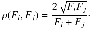$\begin{array}{ccc}\mathit{\rho }\mathrm{\left(}{\mathit{F}}_{\mathit{i}}\mathit{,}{\mathit{F}}_{\mathit{j}}\mathrm{\right)}\mathrm{=}\frac{\mathrm{2}\sqrt{{\mathit{F}}_{\mathit{i}}{\mathit{F}}_{\mathit{j}}}}{{\mathit{F}}_{\mathit{i}}\mathrm{+}{\mathit{F}}_{\mathit{j}}}\mathrm{·}& & \end{array}$(5)On AMBER, the beam unbalance is monitored using dedicated photometric channels, and the consequent visibility loss is largely corrected by the amdlib DRS. Nevertheless, there remains a residual visibility drop because of fast (i.e., faster than the frame integration time) variations in the beam ratio due to wavefront errors, such as high-frequency vibrations of the telescopes. To our knowledge, this residual loss within each frame cannot be corrected for. This effect is also probably chromatic (due to the differential atmospheric refraction affecting the beam injected in the spatial filter, and the dependency of the spatial filter refractive index with wavelength), but we have no analytical law to describe this chromatic behaviour.

These factors depend, of course, on the atmospheric turbulence statistics (seeing and coherence time being the relevant parameters), the air mass and the setup and stability of the instrument as a whole (e.g., telescope vibrations, quality of the coherencing, and cophasing by the fringe tracker, ...). Although it is difficult to attempt describing a very general and accurate statistical perturbation model, we see in the next section that this model describes simple perturbation behaviour that can be exploited in the reduction/calibration process.

3.2. Reduction process

The observations of calibration stars were first reduced with the standard AMBER data reduction software “amdlib” (Tatulli et al. 2007; Malbet et al. 2010) without binning the individual frames. It is known that the squared visibilities estimator provided by amdlib (just as for other ABCD-based⁵ algorithms) is less biased than the estimator of a complex visibility modulus. Therefore, we hereafter work exclusively on squared visibility (V²) data, even though we may occasionally omit the adjective “squared” for readability and when the context is non-ambiguous. Note also that a transformation from the V² estimator to a visibility modulus estimate would not be as trivial as taking the square root of V², because the squared estimator can get negative values due to a bias effect. Following Eq. (1), the reduced $\begin{array}{c}{\mathrm{􏽣}}_{}\\ {\mathit{V}}^{\mathrm{2}}\end{array}$ is then divided by the theoretical squared visibilities $\begin{array}{c}{}_{\mathrm{􏽣}}\\ {\mathit{V}}_{\mathrm{\ast }}^{\mathrm{2}}\end{array}\mathrm{\approx }{\mathit{V}}_{\mathrm{\ast }}^{\mathrm{2}}$ of the corresponding calibration star⁶.

The datasets to be analysed are, thus, composed of a series of calibrated squared visibilities, which represent estimates of the transfer function, with the time sampling of the individual frames.

Whereas an instantaneous drop of visibility may have several causes, which are hardly disentangled, the effect of piston parameters on the dependency of squared visibility with wavelength appears clearly in Eqs. (3) and (4). These two terms can be combined as a global factor. As an example, we can rewrite Eq. (4) as $\begin{array}{ccc}\mathit{\rho }\mathrm{\left(}{\mathit{\sigma }}_{\mathit{p}}\mathit{,}{\mathit{\lambda }}_{\mathit{n}}\mathrm{\right)}\mathrm{\approx }\mathit{C}\mathrm{\left(}{\mathit{\sigma }}_{\mathit{p}}\mathit{,}{\mathit{\lambda }}_{\mathit{m}}\mathrm{\right)}\hspace{0.17em}\mathrm{(}{\left(\mathrm{\Delta }{\mathit{\lambda }}_{\mathit{n}}\right)}^{\mathrm{2}}\mathrm{+}\mathit{a}\hspace{0.17em}\mathrm{\Delta }{\mathit{\lambda }}_{\mathit{n}}\mathrm{)}& & \end{array}$(6)where Δλ_n = λ_n − λ_m with λ_n and λ_m being respectively the nth wavelength and the average wavelength in the considered waveband.

Subtracting the piston effect from the visibilities issued from science object observations is usually not done, as it would either require an accurate knowledge of p and σ_p for each frame or a low-order fit along wavelengths to estimate its amplitude, by following Eqs. (3) and (4). In the latter case, removing that fitted trend would indeed also suppress some actual astrophysical signature included in the squared visibilities. However, it can be used on calibrator observation for the purpose of this study: our “piston-fit corrected” squared visibilities are obtained after subtracting a second order polynomial fit over the spectral dimension for each frame without changing its average squared visibility. Such post-correction of piston effects, illustrated in Fig. 1, is hereafter applied on (and compared with) the squared visibility data reduced in the standard way (i.e., without a correction for the piston and jitter chromatic effect).

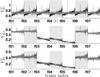Fig. 1 Sample from dataset AT-MR-FT of squared visibilities before (black line) and after (grey) subtraction of a second order polynomial fit representing the effect of the piston and jitter over the spectral dimensions for a few successive frames (f01 to f07, as indicated by the alternation of background colour) and for the three baselines. Each frame displays about 500 spectral channels. The average level of visibility within each frame is conserved. The ⟨s⟩ marker on the abscissa axis indicates a frame included in the “best 20%” selection.

3.3. Distribution of squared visibilities as a function of frame selection

As presented in Table 1, observation data are made of a number of short-exposure frames. Each one contains integrated fringes dispersed along the spectral dimension. Because the quality of each frame depends greatly on the instantaneous turbulence conditions, the data reduction process allows us to select the frames which should actually be used for estimating V², whereas the others have to be discarded. By analysing the distribution of the reduced squared visibilities for all frames and spectral channels, we briefly address the question of the criterion, threshold to be used for that selection, and its impact on the resulting statistics of the visibilities. From which criterion should individual frames be considered valueless and be filtered out? For AMBER data using the standard DRS (Malbet et al. 2010), the default (and advised) criterion is the “fringe S/N”, which is estimated from the residuals of the reduced fringe fitted by an internal calibration fringe frame, and the default threshold is set to the best 20% of the total number of frames, according to that criterion. The user can otherwise choose the selection criterion⁷ and its associated threshold (either absolute or given as a fraction of the total frames).

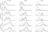Fig. 2 From top to bottom, examples of histograms of $\begin{array}{c}{\mathrm{􏽣}}_{}\\ {\mathit{V}}_{\mathrm{T}}^{\mathrm{2}}\end{array}$ for datasets UT-MR-NoFT, AT-MR-FT and AT-LR-FT. The columns correspond to different threshold levels for the selection of the frames (from left to right: no selection, 60% and 20% of the total number of frames). For each dataset and selection rate, histograms are given with (${\mathit{V}}_{\mathrm{piston}}^{\mathrm{2}}$) and without (${\mathit{V}}_{\mathrm{nopist}}^{\mathrm{2}}$) a correction by a quadratic fit. The grey thin curves a in solid line represent the unselected part of the data.

Figure 2 shows some examples of squared visibility histograms (solid black lines, one exposure file for each dataset) at three different levels of fringe signal-to-noise ratio (S/N) selections with/without the correction of the piston effect. When no selection at all is made (left column), the occurrence of frames with a visibility loss induces distributions, which are wide, possibly asymmetric, and multimodal. The data contain over-represented low-visibility components, ehich appears either as an increased left-side tail or as one or several distinct modes. This latter case appears for observations with the fringe tracker and probably corresponds to a degraded offset (by one or several fringes) or simply lost tracking⁸.

Selecting the frames according to the criterion presented above certainly regularises the distributions, which look closer to a bell-shape (see the second and third columns for two different threshold values). However, this does not seem to allow an unambiguous statistical characterisation from the following considerations:

• 1)

  The mean and standard deviation of the distributions are dependent on the level of frame selection (i.e., the mean increases and the standard deviation decreases for a higher selection threshold) up to a level where they stabilise. The distribution of the observed visibilities are the focus of Sect. 5.2. Unless an appropriately severe selection of frames is made, this means that the resulting sample mean used to estimate V² may yield very different results. On the other hand, throwing away more measurements leads to an increase in the variance of the estimation error. A similar analysis was also tried with other criteria (photometry balance, instantaneous piston,...) with the same threshold dependent behaviour.

• 2)

  The threshold level at which values of the mean and standard deviation stabilise varies greatly with the baseline and ambient conditions. For instance, in some cases, a tolerant selection of 60% gives a distribution which is very similar to that obtained with a conservative selection level of 20%. In such cases, using S/N level that is too high means that 40% of useful data are ignored, although they are available and could be used to better estimate V². In other cases, the 60% criterion is clearly too tolerant and includes data points in the estimation process that may convey more uncertainty than real information about V².

• 3)

  The temporal behaviour of the spectral content is illustrated in Fig. 1 (and more in Fig. 4), where the selected frames at 20% are denoted with a ⟨s⟩ on the abscissa. As mentioned before, the selection uses a S/N criterium to reject a part of the frames. The selected frames have in particular a high mean value and are only slightly affected by the piston effect. It appears, however, that some rejected frames clearly exhibit the same characteristics.

This analysis confirms that it is difficult to automatically derive from a set of observed short-frames the best estimator of the visibility and a reliable related uncertainty (and this justifies the usefulness of having several criteria available for frame selection). However, this also suggests that the frame selection procedure could be adaptive instead of using a fixed criterion, such as S/N. The S/N selection threshold could be increased progressively until the distribution looks stable enough, for instance, on average. The mode of the observed distribution (instead of the sample mean) also appears as an interesting estimator to be investigated⁹. These points deserve a detailed study and are left outside the scope of the present paper.

For each frame, the correction by a quadratic fit compresses the squared visibility around the mean, which reduces the dispersion and makes the different modes more distinguishable on the total distribution (cf., Fig. 2 shows histograms for all frames and wavelengths). This correction mainly affects the analysis of individual frames. The dispersion reduction induced by the correction attenuates the asymmetry, or at least gives a distribution easier to analyse.

4. Differential visibilities

4.1. Construction and associated distributions

In a general way, the colour-differential visibility ΔV is the ratio between the modulus of visibilities at the current spectral channel λ and at a reference channel. The practical choice of the reference channel may vary, depending on the considered instrumental setup and science case. It may be made of a single reference channel or derived from a set of several spectral channels over which the squared visibility is averaged. In addition, it may be fixed (e.g. the continuum around a central spectral feature, such as an emission or absorption line) or variable as a function of the current channel λ. For AMBER data, the standard choice (Millour et al. 2006) is to consider the average from all n_λ observed spectral channels except the current one as the reference.

In the current study, the differential visibility is computed from the same estimator V² (introduced in Sect. 3.2) used for the absolute ones. To compare between these quantities, we therefore work on differential squared visibilities. According to the AMBER convention for the reference channel, these are defined for a current exposure frame i and a given baseline as 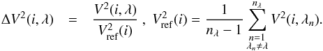$\begin{array}{ccc}\mathrm{\Delta }{\mathit{V}}^{\mathrm{2}}\mathrm{\left(}\mathit{i,\lambda }\mathrm{\right)}& \mathrm{=}& \end{array}$(7)The equation above can be applied at all baselines, frames, and wavelengths. We do not perform a frame selection based on an external criterion here. We only do this for the initial filtering of bad flagged data and an additional filtering process (see Appendix A) to filter out some odd points (usually less than 5% of the total data) with unexpectedly high or low values.

From Eq. (7), it can be seen that the reference squared visibility has a mean value over wavelengths close to the empirical mean value of V² when n_λ is large. The resulting differential squared visibility has, therefore, a mean value close to one, and the corresponding statistical dispersions over wavelengths and over time are also increased by a factor $\mathrm{1}\mathit{/}{\mathit{V}}_{\mathrm{ref}}^{\mathrm{2}}$ with respect to the absolute ones.

Some examples of histograms appear in Fig. 3. When compared to the non-differential squared visibility histograms with the same level of selection (left-hand column of Fig. 2), they indicate that differential visibilities are less scattered, more symmetric, and regular (thus easier to analyse) than their absolute counterparts.

The explanation is that the instantaneous drops, which affect the absolute visibilities, are on a first order and mostly achromatic: for a given frame and baseline, they induce a loss of visibility globally over the spectral band. On a first order approximation, the differential visibility is insensitive to these visibility drops thanks to the normalisation by the reference channel. On a second order only, the dependency of piston and jitter imply a variation in the observed visibility with wavelengths (Eqs. (3) and (4)) on both absolute or differential quantity.

Note that the correction of visibility drop in ΔV² also applies to the frames suffering from an apparent loss (or poor quality) of the fringe tracking in the case of AT-MR-FT observations here: the data corresponding to “secondary modes” located left of the highest-visibility mode (e.g. middle-column plots in Fig. 2) are now integrated in the centred distribution.

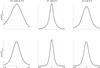Fig. 3 Examples of differential squared visibilities histograms for the same datasets as in the left-hand column of Fig. 2 (no frame selection).

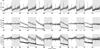Fig. 4 Squared visibilities V2 (black) and rescaled differential squared visibilities $\mathrm{\Delta }{\mathit{V}}_{\mathrm{R}}^{\mathrm{2}}$ (grey) at all three baselines for a small sample of successive frames (indicated by the frame index and the alternation of background colour) from dataset AT-MR-FT and at all wavelengths within each frame. Both quantities are superimposed for frames and baselines, where the visibility is close to ${\mathit{V}}_{\mathrm{m}}^{\mathrm{2}}$, the estimated average squared visibility which is used to rescale ΔV2. The ⟨s⟩ marker on the abscissa axis indicates a frame included in the “best 20%” selection.

4.2. Rescaled differential squared visibilities as an estimator of the squared visibilities

Whereas we presented ΔV² as being normalised by the reference channel, and therefore centred close to one, the observer still needs squared visibilities correctly scaled to the size of the source. A way to obtain this from differential squared visibilities is to rescale them to an average level ${\mathit{V}}_{\mathrm{m}}^{\mathrm{2}}$, which is correctly estimated from the absolute ones. For a given observation file and baseline, the rescaled differential squared visibility is then simply: $\mathrm{\Delta }{\mathit{V}}_{\mathrm{R}}^{\mathrm{2}}\mathrm{\left(}\mathit{i,\lambda }\mathrm{\right)}\mathrm{=}{\mathit{V}}_{\mathrm{m}}^{\mathrm{2}}\hspace{0.17em}\mathrm{\Delta }{\mathit{V}}^{\mathrm{2}}\mathrm{\left(}\mathit{i,\lambda }\mathrm{\right)}$ for any frame i.

Although the actual criterion and threshold for getting that selection remains an open subject of discussion, we nevertheless fixed these parameters by taking the default values mentioned previously (“fringe S/N” criterion with a best 20% frames selection threshold) to make a comparison between the absolute and differential quantities at a same scale. The average for computing ${\mathit{V}}_{\mathrm{m}}^{\mathrm{2}}$ should be both spectral and temporal. We note for the squared visibility at frame i averaged over the spectral channels. The parameter ${\mathit{V}}_{\mathrm{m}}^{\mathrm{2}}$ is the average value of over the set ℐ^s of selected frames: ${\mathit{V}}_{\mathrm{m}}^{\mathrm{2}}\mathrm{=}\mathrm{(}\mathrm{1}\mathit{/}{\mathit{n}}_{\mathrm{\#}\mathrm{\left(}{\mathrm{ℐ}}^{\mathit{s}}\mathrm{\right)}}\mathrm{)}{\sum }_{\mathrm{j}\mathrm{\in }{\mathrm{ℐ}}^{\mathrm{s}}}\mathit{\mu ̅}{}_{{\mathit{v}}^{\mathrm{2}}}\mathrm{\left(}\mathit{j}\mathrm{\right)}$ where n_#(ℐ^s) stands for the number of selected frames.

In Fig. 4 (a small sample from AT-MR-FT data), both quantities are represented linearly for a series of frames and at all wavelengths. Another illustration is shown in Fig. 5, where the frame-averaged levels of V² are at a 20% (${\mathit{V}}_{\mathrm{20}\mathrm{\%}}^{\mathrm{2}}$) selection level and $\mathrm{\Delta }{\mathit{V}}_{\mathrm{R}}^{\mathrm{2}}$ (which is offset here vertically for more clarity) are identical by construction; their global shape along the wavelength is very similar. Howevever, they differ by some weak features and a small slope: $\mathrm{\Delta }{\mathit{V}}_{\mathrm{R}}^{\mathrm{2}}$ is time-averaged over a sample of frames that is much larger than the one used for ${\mathit{V}}_{\mathrm{20}\mathrm{\%}}^{\mathrm{2}}$, and the two samples do not necessarily have the same average piston, which determines the slope of the resulting squared visibilities.

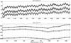Fig. 5 Average values of squared visibilities and rescaled differential squared visibilities with their standard deviations per file for Baseline 1 of our datasets AT-MR-FT (top) and AT-LR-FR (bottom). Squared visibilities are plotted for frame selection levels of 100% and 20% (square and diamond symbols, respectively). Rescaled differential squared visibility $\mathrm{\Delta }{\mathit{V}}_{\mathrm{R}}^{\mathrm{2}}$ (circle) are shifted for more clarity by vertical offsets of 0.1 and were obtained using almost 100% of the frames (see Sect. 4.1). In each case, the lines above and below the average values of squared visibility indicate the values of its standard deviation over one observation file, which are consistent with $\overline{{\mathit{\sigma }}_{\mathit{t}}}$ computed over the whole set of files, as shown in Fig. 6 and in Table 2. This figure is an illustration that shows that differential squared visibility has a very similar shape as the absolute ones but with a lower statistical dispersion.

5. Statistical results

5.1. Compared dispersions

We present and compare hereafter the global statistical results, summarised in Table 2, of different estimators of squared visibility: the empirical mean of squared visibilities¹⁰ at frame selection levels of 100% and 20% (hereafter called ${\mathit{V}}_{\mathrm{100}\mathrm{\%}}^{\mathrm{2}}$ and ${\mathit{V}}_{\mathrm{20}\mathrm{\%}}^{\mathrm{2}}$), and the differential squared visibility rescaled at ${\mathit{V}}_{\mathrm{m}}^{\mathrm{2}}$ ($\mathrm{\Delta }{\mathit{V}}_{\mathrm{R}}^{\mathrm{2}}$) as explained previously. All the quantities in Table 2 are computed separately for each bases and exposure file, and then averaged over the exposures of each dataset.

The first and second columns, ${\mathit{V}}_{\mathrm{m}}^{\mathrm{2}}$ and , indicate the average squared visibility level and the standard deviation of along the selected frames of an exposure file, respectively. We do not discuss in this paper the variations in ${\mathit{V}}_{\mathrm{m}}^{\mathrm{2}}$ between the exposure files or the longer-term variations in the transfer function. As expected from the discussion in Sect. 3.3, ${\mathit{V}}_{\mathrm{m}}^{\mathrm{2}}$ is lower, and is larger for ${\mathit{V}}_{\mathrm{100}\mathrm{\%}}^{\mathrm{2}}$ than for ${\mathit{V}}_{\mathrm{20}\mathrm{\%}}^{\mathrm{2}}$.

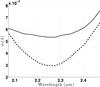Fig. 6 Standard deviation over time of squared visibilities (20% frames selection, solid line) and of rescaled differential squared visibilities (dashed line) for each wavelength per exposure file and for dataset AT-LR-FT. The parameter is averaged over the three baselines and over the different exposure files of the dataset. The lower statistical dispersion of the differential squared visibility compared to the absolute one appears clearly in this figure. The mean values of over wavelengths are presented in Table 2 for all the datasets.

On the other hand, the average squared visibilities of $\mathrm{\Delta }{\mathit{V}}_{\mathrm{R}}^{\mathrm{2}}$ and ${\mathit{V}}_{\mathrm{20}\mathrm{\%}}^{\mathrm{2}}$ are almost identical¹¹ and $\mathit{\sigma ̅}\mathrm{\left(}\mathrm{\Delta }{\mathit{V}}_{\mathrm{R}}^{\mathrm{2}}\mathrm{\right)}$ is almost null: this simply follows the definition of $\mathrm{\Delta }{\mathit{V}}_{\mathrm{R}}^{\mathrm{2}}$ in Sect. 3.3, whose average on each frame is set at ${\mathit{V}}_{\mathrm{m}}^{\mathrm{2}}$. In other words, the differential squared visibilities did not suffer of visibility loss.

The results given hereafter compare the dispersions of both absolute and differential squared visibilities along: 1) the time dimension, which considers all the selected frames within an exposure, the spectral channels which is being considered separately and eventually averaged; and 2) the wavelengths, which are computed after a previous averaging of the squared visibilities from the selected frames within an exposure file.

To compare both the “flatness” over wavelength and the stability over time of the squared visibilities with and without the piston influence as mentioned in Sect. 3.2, the same quantities were also studied after subtraction of a second order polynomial fit in each frame, while conserving their average value (see Fig. 1). These “flattened squared visibilities” statistics are referred hereafter as ${\mathit{V}}_{\mathrm{nopist}\mathit{.}}^{\mathrm{2}}$.

Along the time dimension, the standard deviation per exposure file σ_t can be estimated as the empirical standard deviation per frame divided by the square root of the number of selected frames N_fr within that considered data sample.

The error bars surrounding the curves in Figs. 5 and 6 (for the AT-LR-FT case), show as a function of wavelength for ${\mathit{V}}_{\mathrm{20}\mathrm{\%}}^{\mathrm{2}}$ and $\mathrm{\Delta }{\mathit{V}}_{\mathrm{R}}^{\mathrm{2}}$ without a correction of the piston effect. These numbers are averaged over wavelengths and a baseline and completed by the results for the piston-fitted quantity in Table 2 (respectively columns and $\mathit{\sigma ̅}{}_{\mathit{t}}\mathrm{\left(}{\mathit{V}}_{\mathrm{nopist}}^{\mathrm{2}}\mathrm{\right)}$).

For all the datasets, it appears that the standard deviations over time of the rescaled differential squared visibility $\mathrm{\Delta }{\mathit{V}}_{\mathrm{R}}^{\mathrm{2}}$ are lower than those of the absolute one either with or without frame selection. The improvement factor on is about 25% with respect to the standard ${\mathit{V}}_{\mathrm{20}\mathrm{\%}}^{\mathrm{2}}$ estimator. The frame sample of $\mathrm{\Delta }{\mathit{V}}_{\mathrm{R}}^{\mathrm{2}}$ include relatively more frames of lower quality and more scattered squared visibilities (and thus a higher standard deviation per frame). Since it is also a much larger sample (almost 100% of frames vs. 20%), the standard deviation per file is finally improved; in other terms, the 1/$\sqrt{{\mathit{N}}_{\mathrm{fr}}}$ factor improves the statistical error in favour of the non-selective $\mathrm{\Delta }{\mathit{V}}_{\mathrm{R}}^{\mathrm{2}}$ estimator. Unsurprisingly, the possibility of subtracting a fitted piston effect also induces a significant improvement (between 10% and 30%).

As for the standard deviations , the two right-side columns of Table 2 indicate that the selected squared visibilities ${\mathit{V}}_{\mathrm{20}\mathrm{\%}}^{\mathrm{2}}$ and the rescaled differential visibilities have very comparable scattering along the wavelength dimension.

Note that the rescaling factors, ${\mathit{V}}_{\mathit{m}}^{\mathrm{2}}\mathit{/}\mathit{\mu ̅}{}_{{\mathit{v}}^{\mathrm{2}}}\mathrm{\left(}\mathit{i}\mathrm{\right)}$, applied on each frame to get the differential visibility from the absolute ones are on average >1, which increases the scattering along wavelength. Therefore, we would have $\mathit{\sigma ̅}{}_{\mathit{\lambda }}\mathrm{\left(}\mathrm{\Delta }{\mathit{V}}_{\mathrm{R}}^{\mathrm{2}}\mathrm{\right)}\mathit{>}\mathit{\sigma ̅}{}_{\mathit{\lambda }}\mathrm{\left(}{\mathit{V}}^{\mathrm{2}}\mathrm{\right)}$ if we considered that quantity per frame. (It would also be larger; the computed per frame, note presented in the table, are typically 2 to 3 times higher than the quantities in the two right-side columns of Table 2). As we are discussing here the wavelength scattering computed from the averaged squared visibilities of the considered selected frames, the larger sample of $\mathrm{\Delta }{\mathit{V}}_{\mathrm{R}}^{\mathrm{2}}$ produces a smoother averaging effect than the ${\mathit{V}}_{\mathrm{20}\mathrm{\%}}^{\mathrm{2}}$ sample. Eventually, these two effects appear to balance, and ${\mathit{\sigma }}_{\mathit{\lambda }}\mathrm{\left(}\mathrm{\Delta }{\mathit{V}}_{\mathrm{R}}^{\mathrm{2}}\mathrm{\right)}\mathrm{\approx }{\mathit{\sigma }}_{\mathit{\lambda }}\mathrm{\left(}{\mathit{V}}_{\mathrm{20}\mathrm{\%}}^{\mathrm{2}}\mathrm{\right)}$ over an exposure file.

This applies to either uncorrected or piston-corrected squared visibilities, where the latter quantity has standard deviations reduced by a factor 3 for datasets UT-MR-NoFT and AT-LR-FT but only a marginal gain for the more scattered (and less piston-degraded) dataset AT-MR-FT, as illustrated in Fig. 5.

5.2. Best-fitting distribution laws

5.2.1. Method

We present the results of χ² goodness-of-fit (GoF) tests, which aim at determining whether the empirical distribution of a data sample is compatible or not with a standard distribution with appropriately fitted parameters (Lehmann & Romano 2005). The binary outputs of the tests are obtained according to a predefined probability of false alarm (P_FA) fixed at 5% here.

Below is the list of the statistical laws, which we tested and their associated parameters (μ is the location parameter, σ and η are scales parameters, and ν stands for another possible shape parameter; the expressions of these distributions are recalled in Appendix B):

• normal (), a function of μ and σ;

• Student (t), a function of μ, η and ν_S;

• log-normal (log ), a function of μ and σ; and

• Cauchy (), a function of μ and ν_C.

Let us first remark that this will not be the case for the differential ones even if the squared visibilities are normally distributed. Indeed, the definition of ΔV² in Eq. (7) involves a ratio of normal random variables. It is well known that this ratio leads to a Cauchy distribution (Marsaglia 1965) characterised by the parameters of the two normal distributions involved in the ratio. Between the normal and the Cauchy distributions, the Student distribution is able to fit both a Cauchy distribution (ν_S = 1) and a normal distribution (ν_S → ∞). We note finally that the log-normal distribution was used to fit the distribution of the squared visibilities by Millour et al. (2006).

For the presented χ² tests, the null hypothesis ℋ₀ is that the data is drawn from the tested distribution. The binary result of a test is 0 if the distribution tested under ℋ₀ is accepted and is 1 otherwise. Obviously, even when a data sample is actually drawn from the distribution assumed under ℋ₀, there is always a possibility that the empirical distribution substantially deviates from the distribution under ℋ₀ because of estimation noise caused by the finite number of data samples and by the parameter fitting.

When the GoF test does not involve parameter fitting, results based on asymptotic theory allows us to fix accurately the threshold corresponding to the probability of false alarm (P_FA) (Lehmann & Romano 2005). In Tables 3 and 4, for instance, this threshold was set so that there is a 5% chance that data samples actually drawn from the null distribution are erroneously rejected by a GoF test without fit. This is verified by the second value given in the “Ctrl” lines in the Tables. These values are the rejection rate obtained for data drawn from the tested distribution and contains the same number of samples as the tested interferometric data.

When parameters are estimated in the GoF test, however, the former threshold guarantees a P_FA of 5% that leads to a different rejection rate¹². Assessing analytically the relationship between P_FA and test threshold is much more involved when parameters are estimated, but we can resort to Monte-Carlo simulations to control the actual level of wrong rejections corresponding to the 5% threshold of the case without estimation. The observed values are given by the first values of the “Ctrl” lines in the tables.

5.2.2. Goodness-of-fit results

The results of statistical compatibility tests for the three datasets are presented in Table 3 and for the data corrected from piston and jitter chromatic effects. The numbers represent the observed rejection rates of the null hypothesis and are expressed in percents. A lower value obtained for ${\mathit{V}}_{\mathrm{100}\mathrm{\%}}^{\mathrm{2}}$, ${\mathit{V}}_{\mathrm{20}\mathrm{\%}}^{\mathrm{2}}$ and $\mathrm{\Delta }{\mathit{V}}_{\mathit{R}}^{\mathrm{2}}$ means a higher compatibility with the laws reported in the corresponding columns. The indicative size of the tests can be read in the first value of the “Ctrl” lines.

For the three datasets either with or without a fitted correction of the piston effect, the Student distribution presents the lowest rate of rejection. In particular, the Student law is clearly favoured against the normal distribution when considering the distribution along the wavelength dimension. Along the time dimension, except for the differential squared visibilities, the difference is less pronounced. Even though its rejection rate is relatively lower, the Student law is logically rejected for absolute visibilities without a frame selection for datasets that show a clear asymmetric distribution either due to low visibility level (UT-MR-NoFT) or multimodal behaviour (AT-MR-FT).

Finally, the log-normal and Cauchy laws are most often associated with higher rejection rates than the other two tested distributions. The low-order correction of the piston effect does not modify qualitatively these results and similarly acts in favour of the Student distribution.

These results come in contrast to the generally accepted idea that squared visibilities are normally or log-normally distributed (Millour et al. 2008a). The estimator used to provide the AMBER squared visibilities is actually expressed as a ratio of random variables (Tatulli et al. 2007). This is probably the reason why the Student law, which is a flexible ratio distribution, gives the best fit.

The same analysis was performed on temporally averaged visibilities to characterise their chromatic distribution, as a function of “best S/N” frame percentage. Here, visibilities are averaged over the frames selection set of each exposure file, which corresponds to the way most AMBER users would get their reduced data. Figure 7 represents the GoF rejection rate (in percents) for each threshold value and base from the AT-MR-FT dataset. In accordance with previous non-averaged results, it clearly shows that the Student distribution presents the best fit of averaged data distribution, regardless of the selection threshold.

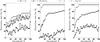Fig. 7 χ2 GoF test applied on average visibilities as a function of the frame selection threshold applied on the AT-MR-FT dataset. The rejection rate is in % and is averaged over exposure files for each baseline.

5.3. Correlations between squared visibilities

How and how much the squared visibilities from different wavelengths are correlated with each other is an important issue for tackling the polychromatic aspect of the inverse problem. Indeed, covariances matrices arise naturally, for instance through the likelihood (Thiébaut 2008; Meimon 2005), but the absence of measures leads in practise to neglect any kind of dependence between the observables.

Between two spectral channels (say, n and p) for a given dataset and baseline, the coefficients of the correlation matrix are $\begin{array}{ccc}\mathrm{c}\hspace{0.17em}\mathrm{\left(}\mathit{n,p}\mathrm{\right)}\mathrm{=}\frac{{⟨\left[{\mathit{V}}_{\mathit{n}}^{\mathrm{2}}\mathrm{-}{\mathrm{⟨}{{\mathit{V}}_{\mathit{n}}^{\mathrm{2}}}^{\mathrm{⟩}}}_{\mathit{t}}\right]\left[{\mathit{V}}_{\mathit{p}}^{\mathrm{2}}\mathrm{-}{\mathrm{⟨}{{\mathit{V}}_{\mathit{p}}^{\mathrm{2}}}^{\mathrm{⟩}}}_{\mathit{t}}\right]⟩}_{\mathit{t}}}{\mathit{\sigma }\mathrm{\left(}{\mathit{V}}_{\mathit{n}}^{\mathrm{2}}\mathrm{\right)}\mathit{\sigma }\mathrm{\left(}{\mathit{V}}_{\mathit{p}}^{\mathrm{2}}\mathrm{\right)}}\mathrm{·}& & \end{array}$(8)This quantity also describes the entries of the sample covariance matrix normalised by the product of the standard deviations, $\mathit{\sigma }\mathrm{\left(}{\mathit{V}}_{\mathit{n}}^{\mathrm{2}}\mathrm{\right)}$ and $\mathit{\sigma }\mathrm{\left(}{\mathit{V}}_{\mathit{p}}^{\mathrm{2}}\mathrm{\right)}$ (therefore c (n,p) = 1 for n = p), as illustrated in Fig. 9.

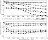Fig. 8 Coefficients of instantaneous correlation between spectral channels, which are averaged over observation files, for the three datasets as a function of the wavelength separation k, expressed in microns. Each curve is issued from a correlations matrix after averaging Eq. (9). Datasets UT-MR-NoFT, AT-MR-FT, and AT-LR-FT are represented, respectively, by circles, diamonds and square symbols (for clarity purposes, only one of each of the 15 correlation points of the two medium-resolution datasets are shown). The squared visibilities with 100% and 20% selection thresholds and the rescaled differential squared visibility appear respectively, as non-filled white, gray and black symbols. Top: without correction of the piston effect. Bottom: after frame-by-frame subtraction of the fitted piston effect.

The coefficients defined by Eq. (8) may be shown as “correlation images” of dimensions [n_λ × n_λ], such as in the examples in Fig. 9. Nevertheless, these results are, on one hand, very much space-consuming (as we want to compare correlations for the different squared visibility estimators, ${\mathit{V}}_{\mathrm{20}\mathrm{\%}}^{\mathrm{2}}$, ${\mathit{V}}_{\mathrm{100}\mathrm{\%}}^{\mathrm{2}}$, and $\mathrm{\Delta }{\mathit{V}}_{\mathrm{R}}^{\mathrm{2}}$, datasets and “piston-correction” options). On the other hand, c (n,p) appears to depend on the wavelength index difference k = n − p (with n>p) rather than on the considered channel p itself.

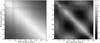Fig. 9 Examples of matrices of the temporal correlation coefficients between spectral channels (see Eq. (8)) for dataset UT-MT-NoFT, averaged over observation files and over the three baselines. Left: ${\mathit{V}}_{\mathrm{20}\mathrm{\%}}^{\mathrm{2}}$, no correction of the piston effect. Right: $\mathrm{\Delta }{\mathit{V}}_{\mathrm{R}}^{\mathrm{2}}$ after piston-fit correction. The value of each correlation coefficient is proportional to the gray scale (far right).

The average instantaneous correlations as a function of the spectral separation k are shown in Fig. 8 for all the squared visibilities and datasets, with and without correction for piston. 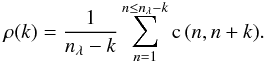$\begin{array}{ccc}\mathit{\rho }\mathrm{\left(}\mathit{k}\mathrm{\right)}\mathrm{=}\frac{\mathrm{1}}{{\mathit{n}}_{\mathit{\lambda }}\mathrm{-}\mathit{k}}\sum _{\mathit{n}\mathrm{=}\mathrm{1}}^{\mathit{n}\mathrm{\le }{\mathit{n}}_{\mathit{\lambda }}\mathrm{-}\mathit{k}}\mathrm{c}\hspace{0.17em}\mathrm{(}\mathit{n,n}\mathrm{+}\mathit{k}\mathrm{)}\mathit{.}& & \end{array}$(9)The squared visibilities without selection (${\mathit{V}}_{\mathrm{100}\mathrm{\%}}^{\mathrm{2}}$) are very much correlated between wavelengths in all cases: this is explained by considering that the sudden visibility losses essentially affect all wavelengths simultaneously and in a similar way.

This effect is very much reduced when considering the selected squared visibilities (${\mathit{V}}_{\mathrm{20}\mathrm{\%}}^{\mathrm{2}}$). The reason is that these frames with a higher S/N are filtered and undergo smaller perturbations (global visibility losses and large pistons) on average. Hence, the correlating effect caused by erratic visibility losses is less pregnant in these frames. It is not the case for the two other dataset and we conclude that some selected frames of UT-MR-NoFT and AT-LR-FT datasets still suffer from visibility loss and pistons at a selection rate of 20%.

Interestingly, sudden visibility losses tend to instantaneously correlate the squared visibilities at all wavelengths, but the piston (with slopes that are either positive or negative along the frames) tends to decorrelate them. This is why the correlation of visibilities increase when the piston is suppressed (bottom figures).

Turning now to the rescaled differential squared visibilities $\mathrm{\Delta }{\mathit{V}}_{\mathrm{R}}^{\mathrm{2}}$, their correlations present a different behaviour. For the $\mathrm{\Delta }{\mathit{V}}_{\mathrm{R}}^{\mathrm{2}}$, the impact of visibility losses between frames is removed by construction, which globally reduces the correlations. Without frame selection, however, the piston effect remains entirely, and the piston is actually a correlating effect for these quantities. Indeed, whatever the slope of the piston, differential squared visibilities at both ends of the spectrum tend to be the opposite side with regard to the average level of the frame. This induces an anticorrelation of differential squared visibilities at large k. Conversely, differential squared visibilities at near wavelengths tend to be on the same side of the average level and thus correlated. When correction for piston is made for $\mathrm{\Delta }{\mathit{V}}_{\mathrm{R}}^{\mathrm{2}}$, this effect is logically reduced.

We may now investigate the cross-correlations c (B_r,B_s) between the squared visibilities from different baselines B_r and B_s with r ≠ s. Those are analysed without considering any shift between the spectral channels (i.e., k = 0). The parameter c (B_r,B_s) is then computed similarly as in Eq. (8), except that r and s refer now to baseline indices and that the averaging operator applies only on frames measured simultaneously on the baselines.

It is difficult to analyse the instantaneous cross correlation between bases for the ${\mathit{V}}_{\mathrm{20}\mathrm{\%}}^{\mathrm{2}}$ because this requires to have simultaneously selected frames (which is usually not the case at a selection rate of 20%).

The results are summarised in Table 5. First, it appears that the correlation depends largely on the considered pair of baseline and that two pairs (here, B₁B₃ and B₂B₃, for which c> 0.2) are much (more) correlated than the third one (B₁B₂, where c ≤ 0.18).

This might translate that some parts of the interferometric chain produce time-variable effects (e.g., a suboptimal adaptive optics a vibrating telescope, turbulences from a longer delay line path, or non-centred beam injection within the optical fiber, etc.) which impact at least one pair of baselines simultaneously through visibility losses and, possibly, through a slope of squared visibilities as a function of wavelengths.

As for how correlations vary in the considered visibility estimator, it appears that the piston-fit subtraction has virtually no effect for squared visibilities ${\mathit{V}}_{\mathrm{100}\mathrm{\%}}^{\mathrm{2}}$. However, its differential counterpart has a lower correlation (40% to 60% for the non-piston corrected case and even lower in the case of piston-fit corrected data).

6. Conclusions and perspectives

This paper provides a detailed statistical analysis framework for interferometric squared visibilities through the example of AMBER’s data. Several conclusions arise from this study.

Regarding squared visibilities, we could see that devising an automatic procedure for optimum threshold selection is difficult. A predetermined S/N selection value might result, depending on the observing conditions, in either a strongly biased sample of frames (whose distribution contains secondary modes, left-wing asymmetry, and/or over-represented tails) or a severe selection, which unnecessarily increases the variance of estimation. We have, however, provided ideas which should be worked out based on the stability of the observed distributions of the frame and on their modes.

Colour-differential squared visibility appears, on the other hand, as a more stable and regular quantity. When rescaled to an average level estimated from a “best frames” sample of the squared visibility, its statistical standard deviation over time is typically improved by 25% with respect to the usual squared visibility estimator, whereas it behaves very similarly along the spectral dimension. This result is because differential squared visibilities allow us to take into account a significantly larger fraction of the data and, thus, benefit from a reduced temporal dispersion. Because of the centring of the rescaled differential squared visibilities of each frame around a common average value, their distribution is also more clearly characterised by the goodness-of-fit test than their absolute counterparts. Re-scaled differential squared visibilities also have a lower spectro-temporal correlation than the absolute ones. Although these results depend very much on the dataset (with different instrumental setups and ambient conditions), they nevertheless indicate that re-scaled differential squared visibilities usually constitute a valuable alternative estimator of squared visibility.

Regarding the statistical law that best describe both V² and $\mathrm{\Delta }{\mathit{V}}_{\mathrm{R}}^{\mathrm{2}}$, we find a better fit for the Student distribution than for others, in particular than the normal distribution. The impact of assuming one or the other of these statistics for model-fitting has been investigated in preliminary work (Schutz et al. 2013) using our AT-MR-FT observations for generating semi-synthetic data (visibilities of a synthetic uniform disk, to which real noise derived from the observations was added). With actual diameters ranging from 0.1 to 20 mas, the accuracy on the estimated diameter is improved (by a factor up to ≈2) by introducing a Student instead of a Gaussian likelihood. This study should be extended to other datasets and source models to assess this effect in a more general context. We finally note that the Student distribution was also used to improve the parameter estimation in model-fitting in Lange et al. (1989) and, more recently, Kazemi & Yatawatta (2013).

We finally find clear correlation effects caused by atmospheric perturbations. Accounting for such correlations should indeed improve the models used in inverse problems and, thus, the accuracy of model fitting and image reconstruction results.

We expect that these results should equally apply to other existing data reduction softwares using either amdlib as their core or a similar ABCD-algorithm, as they would present the same principles and theoretical biases as the official amdlib DRS we used here. On the other hand, a DRS based on Fourier analysis might yield different results, especially on low visibility or poor S/N data. Although such prototype software has already given some significant astrophysical results on the AMBER data (Petrov et al. 2012), it is currently not enough complete nor robust for allowing a numerical comparison on the different cases studied in the present work.

We are planning to extend our analysis to interferometric data obtained from instruments PIONIER (Le Bouquin et al. 2011) and VEGA (Mourard et al. 2009). Finally, a similar statistical study of the closure and differential phases is also under investigation.

References

Appendix A: Aberrant point removing in differential squared visibilities computation

Differential squared visibility histograms which include the original data without any other filters other than the bad flags show that points with very large or low values with respect to the average of 1 may be over-represented compared to the expected “tail” from an usual statistical distribution law, which does not allow to get a realistic fit. The odd statistical points can be caused by a number of observational events (cosmic ray, bad pixel in CCD, etc), which not always corrected or flagged by the data reduction process and not associated with an odd value of a selection criterion (such as the fringe S/N). Thus, they cannot be removed a priori, and we chose to flag and remove them using their own squared visibility value through an iterative process: differential squared visibilities, whose difference from the average exceeds a given threshold (say, 10 times the observed standard deviation σ), are identified by their frame and wavelength number and discarded before computing a new set of differential squared visibilities with its own standard deviation, etc. A stable selection map, which contains more than 95% of the original data, is obtained over just a few of these iterations; the rejection is therefore quantitatively marginal but proved to have significant effects when it comes to fitting a standard distribution law. Such filter maps are used in the analysis proposed in this paper for both differential and absolute squared visibilities as a complement to the standard selection process.

Appendix B: Distributions definition

The normal law: $\begin{array}{ccc}\mathit{f}\mathrm{\left(}\mathit{x}\mathrm{;}\mathit{\mu ,\sigma }\mathrm{\right)}\mathrm{=}\frac{\mathrm{1}}{\mathit{\sigma }\sqrt{\mathrm{2}\mathit{\pi }}}\exp \left[\mathrm{-}\frac{\mathrm{1}}{\mathrm{2}}{\left(\frac{\mathit{x}\mathrm{-}\mathit{\mu }}{\mathit{\sigma }}\right)}^{\mathrm{2}}\right]\mathrm{·}& & \end{array}$The Student law: $\begin{array}{ccc}\mathit{f}\mathrm{\left(}\mathit{x}\mathrm{;}\mathit{\mu ,\sigma ,\nu }\mathrm{\right)}\mathrm{=}\frac{\mathrm{\Gamma }\mathrm{\left(}\mathrm{\right(}\mathit{\nu }\mathrm{+}\mathrm{1}\mathrm{)}\mathit{/}\mathrm{2}\mathrm{)}}{\sqrt{\mathit{\pi \nu }{\mathit{\eta }}^{\mathrm{2}}}\hspace{0.17em}\mathrm{\Gamma }\mathrm{(}\mathit{\nu }\mathit{/}\mathrm{2}\mathrm{)}}{\left(\mathrm{1}\mathrm{+}\frac{{\left(\mathit{x}\mathrm{-}\mathit{\mu }\right)}^{\mathrm{2}}}{\mathit{\nu }{\mathit{\eta }}^{\mathrm{2}}}\right)}^{\mathrm{-}\mathrm{(}\mathit{\nu }\mathrm{+}\mathrm{1}\mathrm{)}\mathit{/}\mathrm{2}}\mathrm{·}& & \end{array}$The log-normal law: $\begin{array}{ccc}\mathit{f}\mathrm{\left(}\mathit{x}\mathrm{;}\mathit{\mu ,\sigma }\mathrm{\right)}\mathrm{=}\frac{\mathrm{1}}{\mathit{x\sigma }\sqrt{\mathrm{2}\mathit{\pi }}}\hspace{0.17em}\exp \left[\mathrm{-}\frac{\mathrm{(}\ln \mathit{x}\mathrm{-}\mathit{\mu }{\mathrm{)}}^{\mathrm{2}}}{\mathrm{2}{\mathit{\sigma }}^{\mathrm{2}}}\right]\mathit{,}\mathit{x}\mathit{>}\mathrm{0.}& & \end{array}$The Cauchy law: $\begin{array}{ccc}\mathit{f}\mathrm{\left(}\mathit{x}\mathrm{;}\mathit{\mu ,\nu }\mathrm{\right)}\mathrm{=}\frac{\mathrm{1}}{\mathit{\pi \nu }\mathrm{[}\mathrm{1}\mathrm{+}{\left(\mathrm{\left(}\mathit{x}\mathrm{-}\mathit{\mu }\mathrm{\right)}\mathit{/}\mathit{\nu }\right)}^{\mathrm{2}}\mathrm{]}}\mathrm{=}\frac{\mathrm{1}}{\mathit{\pi }}\left[\frac{\mathit{\nu }}{\mathrm{(}\mathit{x}\mathrm{-}\mathit{\mu }{\mathrm{)}}^{\mathrm{2}}\mathrm{+}{\mathit{\nu }}^{\mathrm{2}}}\right]\mathrm{·}& & \end{array}$

All Tables

All Figures

Fig. 1 Sample from dataset AT-MR-FT of squared visibilities before (black line) and after (grey) subtraction of a second order polynomial fit representing the effect of the piston and jitter over the spectral dimensions for a few successive frames (f01 to f07, as indicated by the alternation of background colour) and for the three baselines. Each frame displays about 500 spectral channels. The average level of visibility within each frame is conserved. The ⟨s⟩ marker on the abscissa axis indicates a frame included in the “best 20%” selection.

In the text

Fig. 2 From top to bottom, examples of histograms of $\begin{array}{c}{\mathrm{􏽣}}_{}\\ {\mathit{V}}_{\mathrm{T}}^{\mathrm{2}}\end{array}$ for datasets UT-MR-NoFT, AT-MR-FT and AT-LR-FT. The columns correspond to different threshold levels for the selection of the frames (from left to right: no selection, 60% and 20% of the total number of frames). For each dataset and selection rate, histograms are given with (${\mathit{V}}_{\mathrm{piston}}^{\mathrm{2}}$) and without (${\mathit{V}}_{\mathrm{nopist}}^{\mathrm{2}}$) a correction by a quadratic fit. The grey thin curves a in solid line represent the unselected part of the data.

In the text

	Fig. 3 Examples of differential squared visibilities histograms for the same datasets as in the left-hand column of Fig. 2 (no frame selection).
In the text

Fig. 4 Squared visibilities V2 (black) and rescaled differential squared visibilities $\mathrm{\Delta }{\mathit{V}}_{\mathrm{R}}^{\mathrm{2}}$ (grey) at all three baselines for a small sample of successive frames (indicated by the frame index and the alternation of background colour) from dataset AT-MR-FT and at all wavelengths within each frame. Both quantities are superimposed for frames and baselines, where the visibility is close to ${\mathit{V}}_{\mathrm{m}}^{\mathrm{2}}$, the estimated average squared visibility which is used to rescale ΔV2. The ⟨s⟩ marker on the abscissa axis indicates a frame included in the “best 20%” selection.

In the text

Fig. 5 Average values of squared visibilities and rescaled differential squared visibilities with their standard deviations per file for Baseline 1 of our datasets AT-MR-FT (top) and AT-LR-FR (bottom). Squared visibilities are plotted for frame selection levels of 100% and 20% (square and diamond symbols, respectively). Rescaled differential squared visibility $\mathrm{\Delta }{\mathit{V}}_{\mathrm{R}}^{\mathrm{2}}$ (circle) are shifted for more clarity by vertical offsets of 0.1 and were obtained using almost 100% of the frames (see Sect. 4.1). In each case, the lines above and below the average values of squared visibility indicate the values of its standard deviation over one observation file, which are consistent with $\overline{{\mathit{\sigma }}_{\mathit{t}}}$ computed over the whole set of files, as shown in Fig. 6 and in Table 2. This figure is an illustration that shows that differential squared visibility has a very similar shape as the absolute ones but with a lower statistical dispersion.

In the text

Fig. 6 Standard deviation over time of squared visibilities (20% frames selection, solid line) and of rescaled differential squared visibilities (dashed line) for each wavelength per exposure file and for dataset AT-LR-FT. The parameter is averaged over the three baselines and over the different exposure files of the dataset. The lower statistical dispersion of the differential squared visibility compared to the absolute one appears clearly in this figure. The mean values of over wavelengths are presented in Table 2 for all the datasets.

In the text

	Fig. 7 χ2 GoF test applied on average visibilities as a function of the frame selection threshold applied on the AT-MR-FT dataset. The rejection rate is in % and is averaged over exposure files for each baseline.
In the text

Fig. 8 Coefficients of instantaneous correlation between spectral channels, which are averaged over observation files, for the three datasets as a function of the wavelength separation k, expressed in microns. Each curve is issued from a correlations matrix after averaging Eq. (9). Datasets UT-MR-NoFT, AT-MR-FT, and AT-LR-FT are represented, respectively, by circles, diamonds and square symbols (for clarity purposes, only one of each of the 15 correlation points of the two medium-resolution datasets are shown). The squared visibilities with 100% and 20% selection thresholds and the rescaled differential squared visibility appear respectively, as non-filled white, gray and black symbols. Top: without correction of the piston effect. Bottom: after frame-by-frame subtraction of the fitted piston effect.

In the text

Fig. 9 Examples of matrices of the temporal correlation coefficients between spectral channels (see Eq. (8)) for dataset UT-MT-NoFT, averaged over observation files and over the three baselines. Left: ${\mathit{V}}_{\mathrm{20}\mathrm{\%}}^{\mathrm{2}}$, no correction of the piston effect. Right: $\mathrm{\Delta }{\mathit{V}}_{\mathrm{R}}^{\mathrm{2}}$ after piston-fit correction. The value of each correlation coefficient is proportional to the gray scale (far right).

In the text

References

- Chesneau, O., Nardetto, N., Millour, F., et al. 2007, A&A, 464, 119 [NASA ADS] [CrossRef] [EDP Sciences] [Google Scholar]
- Colavita, M. M. 1999, PASP, 111, 111 [NASA ADS] [CrossRef] [Google Scholar]
- Cornwell, T. J. 1987, A&A, 180, 269 [NASA ADS] [Google Scholar]
- Eisenhauer, F., Perrin, G., Straubmeier, C., et al. 2007, Proc. IAU, null, 100 [Google Scholar]
- Hanot, C., Mennesson, B., Martin, S., et al. 2011, ApJ, 729, 110 [NASA ADS] [CrossRef] [Google Scholar]
- Kazemi, S., & Yatawatta, S. 2013, MNRAS, 435, 597 [NASA ADS] [CrossRef] [Google Scholar]
- Labeyrie, A. 1975, ApJ, 196, L71 [NASA ADS] [CrossRef] [Google Scholar]
- Lange, K. L., Little, R. J. A., & Taylor, J. M. G. 1989, J. Am. Stat. Assoc., 84, 881 [Google Scholar]
- Le Bouquin, J.-B., Berger, J.-P., Lazareff, B., et al. 2011, A&A, 535, A67 [NASA ADS] [CrossRef] [EDP Sciences] [Google Scholar]
- Lehmann, E. L., & Romano, J. P. 2005, Testing statistical hypotheses, 3rd edn., Springer Texts in Statistics (New York: Springer) [Google Scholar]
- Lopez, B., Antonelli, P., Wolf, S., et al. 2009, in SPIE, Marseille, France, 1 [Google Scholar]
- Malbet, F., Duvert, G., Millour, F. A., et al. 2010, in SPIE Conf. Ser., 7734 [Google Scholar]
- Marsaglia, G. 1965, j-J-AM-STAT-ASSOC, 60, 193 [Google Scholar]
- Meilland, A., Millour, F., Stee, P., et al. 2007, A&A, 464, 73 [NASA ADS] [CrossRef] [EDP Sciences] [Google Scholar]
- Meimon, S. 2005, Reconstruction d’images astronomiques en interférométrie optique [Google Scholar]
- Millour, F. 2006, Interférométrie différentielle avec AMBER [Google Scholar]
- Millour, F., Vannier, M., Petrov, R., et al. 2006, EAS Pub. Ser., 22, 379 [CrossRef] [EDP Sciences] [Google Scholar]
- Millour, F., Petrov, R., Malbet, F., et al. 2008a, in 2007 ESO Instrument Calibration Workshop, eds. A. Kaufer, & F. Kerber, 461 [Google Scholar]
- Millour, F., Valat, B., Petrov, R. G., & Vannier, M. 2008b, in SPIE Conf. Ser., 7013 [Google Scholar]
- Mourard, D., Tallon-Bosc, I., Rigal, F., et al. 1994, A&A, 288, 675 [NASA ADS] [Google Scholar]
- Mourard, D., Clausse, J. M., Marcotto, A., et al. 2009, A&A, 508, 1073 [NASA ADS] [CrossRef] [EDP Sciences] [Google Scholar]
- Perrin, G. 2003, A&A, 400, 1173 [NASA ADS] [CrossRef] [EDP Sciences] [Google Scholar]
- Petrov, R. G., Malbet, F., Richichi, A., et al. 2000, in SPIE Conf. Ser. 4006, eds. P. Léna, & A. Quirrenbach, 68 [Google Scholar]
- Petrov, R. G., Millour, F., Lagarde, S., et al. 2012, in SPIE Conf. Ser., 8445 [Google Scholar]
- Roddier, F. 1986, Opt. Commun., 60, 145 [Google Scholar]
- Roddier, F., & Lena, P. 1984, J. Optics, 15, 171 [NASA ADS] [CrossRef] [Google Scholar]
- Schutz, A., Vannier, M., Mary, D., & Ferrari, A. 2013, in 24th GRETSI Symp. [Google Scholar]
- Tallon-Bosc, I., Tallon, M., Thiébaut, E., et al. 2008, in SPIE Conf. Ser., 7013 [Google Scholar]
- Tatulli, E., Millour, F., Chelli, A., et al. 2007, A&A, 464, 29 [NASA ADS] [CrossRef] [EDP Sciences] [Google Scholar]
- Thiébaut, E. 2008, in Astronomical Telescopes and Instrumentation, Proc. SPIE, 70131I–70131I–12 [Google Scholar]