| Issue |
A&A
Volume 565, May 2014
|
|
|---|---|---|
| Article Number | A26 | |
| Number of page(s) | 18 | |
| Section | Extragalactic astronomy | |
| DOI | https://doi.org/10.1051/0004-6361/201220703 | |
| Published online | 28 April 2014 | |
Two active states of the narrow-line gamma-ray-loud AGN GB 1310+487
1 Max-Planck-Institut für Radioastronomie, Auf dem Hügel 69, 53121 Bonn, Germany
e-mail: This email address is being protected from spambots. You need JavaScript enabled to view it.
2 Astro Space Center of Lebedev Physical Institute, Profsoyuznaya Str. 84/32, 117997 Moscow, Russia
3 Sternberg Astronomical Institute, Moscow State University, Universitetskii pr. 13, 119992 Moscow, Russia
4 Department of Physics and Astronomy, University of New Mexico, Albuquerque NM, 87131, USA
5 Hiroshima Astrophysical Science Center, Hiroshima University, 1-3-1, Kagamiyama, Higashi-Hiroshima, 739-8526 Hiroshima, Japan
6 INAF/IASF–Bologna, via Gobetti 101, 40129 Bologna, Italy
7 Instituto Nacional de Astrofisica, Optica y Electronica, Tonantzintla, Puebla, CP 72860 Mexico, Mexico
8 Department of Astronomy, University of California, Berkeley, CA 94720-3411, USA
9 NASA/Goddard Space Flight Center, Greenbelt, MD 20771, USA
10 National Research Council Research Associate, National Academy of Sciences, Washington, DC 20001, resident at Naval Research Laboratory, Washington, DC 20375, USA
11 Dip. di Fisica, Universitá degli Studi di Perugia, via A. Pascoli, 060123 Perugia, Italy
12 INFN – Sezione di Perugia, via A. Pascoli, 06123 Perugia, Italy
13 INAF-IRA Bologna, Via Gobetti 101, 40129 Bologna, Italy
14 Université Bordeaux 1, CNRS/IN2p3, Centre d’Études Nucléaires de Bordeaux Gradignan, 33175 Gradignan, France
15 Laboratoire Leprince-Ringuet, École polytechnique, CNRS/IN2P3, 91120 Palaiseau, France
16 U.S. Naval Research Laboratory, Code 7653, 4555 Overlook Ave. SW, Washington, DC 20375-5352, USA
17 Department of Physical Sciences, Hiroshima University, Higashi- Hiroshima, Hiroshima 739-8526, Japan
18 Department of Physics, Stanford University, Stanford, CA 94305, USA
19 Department of Astronomy, Stockholm University, 106 91 Stockholm, Sweden
20 The Oskar Klein Centre for Cosmoparticle Physics, AlbaNova, 106 91 Stockholm, Sweden
21 Department of Physics, Stockholm University, AlbaNova, 106 91 Stockholm, Sweden
22 Department of Physics, Purdue University, 525 Northwestern Ave, West Lafayette, IN 47907, USA
23 Univ. Bordeaux, CENBG, UMR 5797, 33170 Gradignan, France
24 CNRS, IN2P3, CENBG, UMR 5797, 33170 Gradignan, France
25 Cahill Center for Astronomy andAstrophysics, California Institute of Technology, 1200 E. California Blvd., Pasadena, CA 91101, USA
26 ASI–ASDC, via G. Galilei, 00044 Frascati, Roma, Italy
27 Nordic Optical Telescope, Apdo. de Correos 474, 38700 Santa Cruz de la Palma, Spain
28 Pulkovo Observatory, Pulkovskoe Chaussee 65/1, 196140 St. Petersburg, Russia
29 Crimean Astrophysical Observatory, 98409 Nauchny, Crimea, Ukraine
30 Instituto Radioastronomía Milimétrica„ Avenida Divina Pastora 7, Local 20, 18012, Granada, Spain
31 Department of Astronomy, Kyoto University, Kitashirakawa-Oiwake-cho, Sakyo-ku, 606-8502 Kyoto, Japan
32 INAF/IASF–Palermo, via U. La Malfa 153, 90146 Palermo, Italy
33 Kwasan Observatory, Kyoto University, Ohmine-cho Kita Kazan, Yamashina-ku, 607-8471 Kyoto, Japan
Received: 7 November 2012
Accepted: 8 January 2014
Abstract
Context. Previously unremarkable, the extragalactic radio source GB 1310+487 showed a γ-ray flare on 2009 November 18, reaching a daily flux of ~ 10-6 photons cm-2 s-1 at energies E> 100 MeV and became one of the brightest GeV sources for about two weeks. Its optical spectrum shows strong forbidden-line emission while lacking broad permitted lines, which is not typical for a blazar. Instead, the spectrum resembles those of narrow emission-line galaxies.
Aims. We investigate changes in the object’s radio-to-GeV spectral energy distribution (SED) during and after the prominent γ-ray flare with the aim of determining the nature of the object and of constraining the origin of the variable high-energy emission.
Methods. The data collected by the Fermi and AGILE satellites at γ-ray energies; Swift at X-ray and ultraviolet (UV); the Kanata, NOT, and Keck telescopes at optical; OAGH and WISE at infrared (IR); and IRAM 30 m, OVRO 40 m, Effelsberg 100 m, RATAN-600, and VLBA at radio are analyzed together to trace the SED evolution on timescales of months.
Results. The γ-ray/radio-loud narrow-line active galactic nucleus (AGN) is located at redshift z = 0.638. It shines through an unrelated foreground galaxy at z = 0.500. The AGN light is probably amplified by gravitational lensing. The AGN SED shows a two-humped structure typical of blazars and γ-ray-loud narrow-line Seyfert 1 galaxies, with the high-energy (inverse-Compton) emission dominating by more than an order of magnitude over the low-energy (synchrotron) emission during γ-ray flares. The difference between the two SED humps is smaller during the low-activity state. Fermi observations reveal a strong correlation between the γ-ray flux and spectral index, with the hardest spectrum observed during the brightest γ-ray state. The γ-ray flares occurred before and during a slow rising trend in the radio, but no direct association between γ-ray and radio flares could be established.
Conclusions. If the γ-ray flux is a mixture of synchrotron self-Compton and external Compton emission, the observed GeV spectral variability may result from varying relative contributions of these two emission components. This explanation fits the observed changes in the overall IR to γ-ray SED.
Key words: quasars: individual: GB 1310+487 / galaxies: jets / gamma rays: galaxies / radiation mechanisms: non-thermal / galaxies: active
© ESO, 2014
1. Introduction
Blazars are active galactic nuclei (AGNs) in which relativistically beamed emission from the jet dominates the radiative output across most of the electromagnetic spectrum. The spectral energy distribution (SED) of a blazar has two broad components: one peaking between far-IR and X-ray wavelengths and the other peaking at γ-rays (Abdo et al. 2010b). The low-energy emission component is believed to be dominated by synchrotron radiation of relativistic electrons/positrons in the jet. Radiation at higher energies could be due to the inverse-Compton scattering of synchrotron photons emitted by the electrons themselves (synchrotron self-Compton process, SSC; e.g., Jones et al. 1974; Ghisellini & Maraschi 1989; Marscher & Travis 1996) and/or photons from external sources (external Compton process, EC; e.g., Sikora et al. 1994; Dermer & Schlickeiser 2002). The sources of the external seed photons for the EC process include the accretion disk, broad-line region (BLR) clouds, warm dust (dusty torus), synchrotron emission from other faster/slower regions of the jet, and the cosmic microwave background (CMB), with their relative contributions varying for different objects. The models based on inverse-Compton scattering by relativistic electrons are generally referred to as leptonic models (Celotti & Ghisellini 2008; Ghisellini & Tavecchio 2009; Boettcher 2010, 2012). An alternative view regarding the origin of blazar high-energy emission is represented by hadronic models (Mücke & Protheroe 2001; Mücke et al. 2003; Sikora 2011), where relativistic protons in the jet are the primary accelerated particles. We adopt the leptonic models as the basis for the following discussion.
Two types of radio-loud AGNs give rise to the blazar phenomenon: flat-spectrum radio quasars (FSRQs) and BL Lacertae-type objects (BL Lacs). Flat-spectrum radio quasars are characterized by high luminosities, prominent broad emission lines in their optical spectra, and the peak of synchrotron jet emission occurring at mid- or far-IR wavelengths. Thermal emission, probably originating in the accretion disk surrounding the central black hole, may contribute a significant fraction of the optical and UV emission in some FSRQs (Villata et al. 2006; Jolley et al. 2009; Abdo et al. 2010a). BL Lacertae-type objects, on the other hand, show mostly featureless optical spectra dominated by the nonthermal continuum produced by a relativistic jet. Their synchrotron emission peak is located between far-IR and hard-X-ray energies (Padovani & Giommi 1995; Fossati et al. 1998; Ghisellini et al. 1998). In GeV γ-rays, BL Lacs show a wide distribution of spectral slopes, while FSRQs almost exclusively exhibit soft γ-ray spectra (Abdo et al. 2010c). It is not clear whether there is a physical distinction between BL Lacs and FSRQs, or if they represent two extremes of a continuous distribution of AGN properties such as black hole mass (M•), spin, or accretion rate (Ghisellini et al. 2011). Recently, five radio-loud narrow-line Seyfert 1 galaxies (NLSy1s) have been detected in γ-rays by Fermi/LAT, suggesting the presence of a new class of γ-ray-emitting AGNs (Abdo et al. 2009d; D’Ammando et al. 2012). The relationship between NLSy1 and blazars is under debate. It has been suggested that radio-loud NLSy1 galaxies harbor relativistic jets (Foschini 2013; D’Ammando et al. 2013), but unlike blazars they are powered by less massive black holes hosted by spiral galaxies (Yuan et al. 2008; Komberg & Ermash 2013). The presence of a relativistic jet is supported by observation of superluminal motions in the parsec-scale radio jet of the NLSy1 SBS 0846+513 (D’Ammando et al. 2012). The observational evidence that radio-loud NLSy1 have M• smaller than those of blazars has recently been challenged by Calderone et al. (2013). Some nearby radio galaxies including Cen A (NGC 5128), Per A (NGC 1275, 3C 84), and Vir A (M87, 3C 274) are detected by Fermi/LAT (Abdo et al. 2010j). While part of their γ-ray luminosity is attributed to inverse-Compton scattering of CMB photons on the extended (kpc-scale) radio lobes of the galaxies (Cheung 2007; Abdo et al. 2010i), contribution from the core region is also evident (Abdo et al. 2009b, 2010h). Unlike other radio galaxies studied by Abdo et al. (2010j), Per A exhibits episodes of rapid GeV variability (Donato et al. 2010; Ciprini 2013). The core γ-ray emission in radio galaxies is probably produced by the same mechanisms as in blazars, but with less extreme relativistic beaming.
Since early satellite observations established the association of some discrete γ-ray sources with AGNs, it became clear that blazars emit a considerable fraction of their total energy output above 100 MeV (Swanenburg et al. 1978; Hartman et al. 1999; Mukherjee 2002). The current generation of space-based γ-ray telescopes that use solid-state (silicon) detectors is represented by instruments onboard AGILE (Tavani et al. 2009, 2008) and Fermi (Atwood et al. 2009), which open a window into the world of GeV variability and spectral behavior of γ-ray-loud AGNs. In contrast to previous expectations (Vercellone et al. 2004), most of the brightest γ-ray blazars detected by Fermi and AGILE were already known from the EGRET era (Tavani 2011). On the other hand, many blazars previously unknown as γ-ray emitters were observed to reach high fluxes (>10-6 photons cm-2 s-1 at energies E> 100 MeV) for only a short period of time during a flare. In this work, we present a detailed investigation of one such object.
The radio source GB 1310+487 (also known as GB6 B1310+48441, and CGRaBS J1312+4828, listed in the Fermi γ-ray source catalogues as 1FGL J1312.4+4827 (Abdo et al. 2010d) and 2FGL J1312.8+4828 (Nolan et al. 2012), radio VLBI position2αJ2000 = 13h12m43.s353644 ± 0.22 mas,  mas (Beasley et al. 2002)) is a flat-spectrum radio source. It was unremarkable among other faint γ-ray detected blazars (the E> 100 MeV flux during the first 11 months of the Fermi mission was ~ 3 × 10⁻⁸ photons cm-2 s-1, as reported in the 1FGL catalogue; Abdo et al. 2010d) until it appeared in the daily Fermi sky with a flux of ~ 1.0 × 10⁻⁶ photons cm-2 s-1 on 2009 November 183 (Sokolovsky et al. 2009). AGILE observations reported two days later confirmed the high-flux state of the source (Bulgarelli et al. 2009). Follow-up observations in the near-IR (Carrasco et al. 2009) and optical (Itoh et al. 2009) also found GB 1310+487 in a high state compared to historical records. The daily average γ-ray flux remained at ~ 1.0 × 10⁻⁶ photons cm-2 s-1 for more than a week (Hays & Escande 2009).
This paper presents multiwavelength observations of GB 1310+487 before, during, and after its active γ-ray state, and suggests possible interpretations of the observed SED evolution. In Sect. 2 we describe the observing techniques and data analysis. Section 3 presents an overview of the observational results. In Sect. 4 we discuss their implications, and we summarize our findings in Sect. 5. Throughout this paper, we adopt the following convention: the spectral index α is defined through the energy flux density as a function of frequency Fν ∝ ν+ α, the photon index Γph is defined through the number of incoming photons as a function of energy dN(E)/dE ∝ E− Γph, and the two indices are related by Γph = 1 − α. We use a ΛCDM cosmology, with the following values for the cosmological parameters: H0 = 71 km s-1 Mpc-1, Ωm = 0.27, and ΩΛ = 0.73 (see Komatsu et al. 2009; Hogg 1999), which corresponds to a luminosity distance of DL = 3800 Mpc, an angular-size distance of DA = 1400 Mpc, and a linear scale of 6.9 pc mas-1 at the source redshift z = 0.638 (see Sect. 3.4).
2. Multiwavelength observations
2.1. Gamma-ray observations with Fermi/LAT
Fermi Gamma-ray Space Telescope (FGST, hereafter Fermi) is an orbiting observatory launched on 2008 June 11 by a Delta II rocket from the Cape Canaveral Air Force Station in Florida, USA. The main instrument aboard Fermi is the Large Area Telescope (LAT; Atwood et al. 2009; Abdo et al. 2009a; Ackermann et al. 2012), a pair-conversion telescope designed to cover the energy band from 20 MeV to greater than 300 GeV. The Fermi/LAT is providing a unique combination of high sensitivity and a wide field of view of about 60°. Fermi is operated in an all-sky survey mode most of the time, which makes it ideal for monitoring AGN variability.
The dataset reported here was collected during the first 33 months of Fermi science observations from 2008 August 4 to 2011 June 13 in the energy range 100 MeV–100 GeV. The 33 month time interval is divided into subintervals according to the level of its γ-ray activity as observed by Fermi/LAT (see Table 1).
Fermi/LAT data comprise a database containing arrival times, directions, and energies of individual silicon-tracker events supplemented by information about the spacecraft position and attitude needed to calculate the effective exposure for a celestial region and time interval of interest. The maximum-likelihood method is used to analyze these data by constructing an optimal model of the sky region as a combination of point-like and diffuse sources having a spectrum associated with each one of them (Mattox et al. 1996; Abdo et al. 2010d). The significance of source detection is quantified by the Test Statistic (TS) value, determined by taking twice the logarithm of the likelihood ratio between the models including the target source (L1) and one including only the background sources (L0): TS ≡ 2(lnL1 − lnL0). The ratios L0 and L1 are maximized with respect to the free parameters in the models. The Monte-Carlo simulation performed by Mattox et al. (1996) for EGRET confirmed theoretical predictions (Wilks 1938) that for a GeV telescope, in most cases, the TS distribution is close to χ2.
The unbinned likelihood analysis was performed with the Fermi Science Tools package4 version v9r21p0. The DIFFUSE class events in the energy range 100 MeV–100 GeV were extracted from a region of interest defined as a circle of 15deg radius centered at the radio position of GB 1310+487. A cut on zenith angle >100° was applied to reduce contamination from Earth-limb γ-rays, produced by cosmic rays interacting with the upper atmosphere (Shaw et al. 2003; Abdo et al. 2009c). Observatory rocking angles of greater than 52deg were also excluded. A set of instrument response functions (IRFs) P6_V11_DIFFUSE was used in the analysis. The sky model contained point sources from the 2FGL catalogue (Nolan et al. 2012) within 20deg from the target, as well as Galactic gll_iem_v02_P6_V11_DIFFUSE.fit and isotropic isotropic_iem_v02_P6_V11_DIFFUSE.txt diffuse components5. All point-source spectra were modeled with a power law; the photon index was fixed to the catalogue value for all sources except the target. The diffuse-background parameters were not fixed. The estimated systematic uncertainty of flux measurements with LAT using P6_V11 IRFs is 10% at 100 MeV, 5% at 500 MeV, and 20% at 10 GeV and above6.
The lightcurve of the target source was constructed by applying the above analysis technique to a number of independent time bins. The time bin width was chosen to be seven days. Sources with less than one photon detected in the individual bin or with TS < 25 were excluded from the sky model for that bin. The lightcurves were computed by integrating the power-law model in the energy range 100 MeV–100 GeV.
For lightcurves with time bins of fixed widths, the choice of bin width is a compromise between temporal resolution and signal-to-noise ratio (S/N) for the individual bins. For Fermi/LAT an alternative method has recently been developed (Lott et al. 2012), in which the time bin widths are flexible and chosen to produce bins with constant flux uncertainty. Flux estimates are still produced with the standard LAT analysis tools. In this case we used Fermi Science Tools v9r27p1 and P7CLEAN_V6 event selection and IRFs, for which the current version of the adaptive binning method has been optimized (we have checked that using the P7SOURCE_V6 class yields very similar fluxes). At times of high source flux, the time bins are narrower than during lower flux levels, therefore allowing us to study more rapid variability during these periods.
The lower energy limit of the integral fluxes computed for the adaptively binned lightcurve is chosen to minimize the bin widths needed to reach the desired relative flux uncertainty for most bins. The derivation of this energy limit, called the optimum energy, is presented by Lott et al. (2012). Because the source is variable and the optimum energy value depends on the flux, we compute the optimum energy with the average flux over the first two years of LAT operation reported in the 2FGL catalogue (Nolan et al. 2012). The optimum energy is found to be E0 = 283 MeV for this source. We produced two sets of adaptively binned lightcurves in the 283 MeV–200 GeV energy range, one with 25% flux uncertainties and another with 15% uncertainties. For each of these uncertainty levels we created a second version of the lightcurve by performing the adaptive binning in the reverse-time direction.
Changes in the γ-ray spectrum between time intervals considered in the analysis.
Swift observations of GB 1310+487.
2.2. Gamma-ray observations with AGILE/GRID
The AGILE γ-ray satellite (Tavani et al. 2009, 2008) was launched on 2007 April 23 by a PSLV rocket from the Satish Dhawan Space Centre at Sriharikota, India. AGILE is a mission of the Italian Space Agency (ASI) devoted to high-energy astrophysics, and is currently the only space mission capable of observing cosmic sources simultaneously in the energy bands 18–60 keV and 30 MeV–30 GeV thanks to its two scientific instruments: the hard X-ray Imager (Super-AGILE; Feroci et al. 2007) and the Gamma-Ray Imaging Detector (GRID; Rappoldi et al. 2009). During the first two years of the mission, AGILE was mainly operated by performing 2–4 week-long pointed observations, but following the reaction wheel malfunction in October 2009 it was operated in a spinning observing mode, surveying a large fraction of the sky each day.
The AGILE/GRID instrument detected enhanced γ-ray emission from GB 1310+487from 2009 November 20 17:00 (JD 2 455 156.2) to 2009 November 22 17:00 (JD 2 455 158.2) (see Bulgarelli et al. 2009, for preliminary results). Level 1 AGILE/GRID data were reanalyzed using the AGILE Standard Analysis Pipeline (see Pittori et al. 2009; Vercellone et al. 2010, for a description of the AGILE data reduction). We used γ-ray events from the ASDCSTDe archive, filtered by means of the FM3.119 pipeline. Counts, exposure, and Galactic background γ-ray maps were created with a bin size of 0.°5 × 0.°5 , for E ≥ 100 MeV. Since AGILE was in its spinning observing mode, all maps were generated including all events collected up to 50° off-axis. We rejected all γ-ray events whose reconstructed directions form angles with the satellite-Earth vector smaller than 90°, reducing the γ-ray Earth limb contamination by excluding regions within ~ 20° from the Earth limb. We used the latest version (BUILD-20) of the Calibration files (I0023), which will be publicly available at the ASI Science Data Centre (ASDC) site7, and the γ-ray diffuse emission model (Giuliani et al. 2004). We subsequently ran the AGILE Multi-Source Maximum Likelihood Analysis (ALIKE) task using a radius of analysis of 10° in order to obtain the position and the flux of the source. A power-law spectrum with a photon index Γ = 2.1 was assumed in the analysis.
2.3. X-ray observations with Swift/XRT
The X-ray Telescope (XRT; Burrows et al. 2005) onboard the Swift satellite (Gehrels et al. 2004) provides simultaneous imaging and spectroscopic capability over the 0.2–10 keV energy range. The source GB 1310+487 was observed by Swift at seven epochs during the two γ-ray activity periods and in June 2011 during the low post-flare state. A summary of the Swift observations is presented in Table 2. Swift/XRT was operated in photon-counting (pc) mode during all observations. The low count rate of the source allows us to neglect the pile-up effect which is of concern for the XRT in pc mode if the count rate8 is ≥0.6 count s-1.
The xrtpipeline task from the HEASoft v6.14 package was used for the data processing with the standard filtering criteria. To increase the number of counts for spectral analysis, the resulting event files were combined with xselect to produce average X-ray spectra for the periods of Flare 1 and Flare 2 defined in Table 1. The spectrum for the Flare 1 period was binned to contain at least 25 counts per bin to utilize the χ2 minimization technique. The combined spectra were analyzed with XSPEC v12.8.1. The simple absorbed power-law model with the H I column density fixed to the Galactic value NH I = 0.917 × 1020 cm-2 (obtained from radio 21 cm measurements by Kalberla et al. 2005) provided a statistically acceptable fit (reduced χ2 = 1.2 for 12 degrees of freedom) to the 0.3–10 keV spectrum. Leaving NH I free to vary results in the values NH I = 0.4 − 0.5 × 1022 cm-2 and Γph X - ray ~ 1.3. However, this model does not improve the fits. The low photon counts prevent a more detailed study.
Individual observations obtained during the periods of Flare 1 and Flare 2 were also analyzed using the same fixed–NH I model, but no evidence of spectral variability within the periods was found; however, the low photon counts could easily hide mild spectral changes. The Swift/XRT observation obtained during the Flare 2 and post-flare intervals (Table 1) resulted in a low number of detected photons. The Cash (1979) statistic is applied to fit this dataset with the absorbed power-law model. The Cash statistic is based on a likelihood ratio test and is widely used for parameter estimation in photon-counting experiments. The net count rate in the 0.3–10 keV energy range changed by a factor of 1.6 between the two observations conducted during Flare 1 and by a factor of 3.5 over the whole 33-month period. The X-ray spectral analysis results are presented in Table 2.
2.4. Ultraviolet-optical observations
The Swift Ultraviolet-Optical Telescope (UVOT; Roming et al. 2005) has a diameter of 0.3 m and is equipped with a microchannel-plate intensified CCD detector operated in photon-counting mode. Swift/UVOT observed GB 1310+487 simultaneously with Swift/XRT. Various filters were used at different epochs ranging from the U to M2 bands (as detailed in Table 2), with the best coverage achieved in the U band. Since the object is very faint, multiple subexposures taken during each observation were stacked together with the tool uvotimsum from the HEASoft package. A custom-made script based on uvotsource was employed for aperture photometry (using the standard 5′′ aperture diameter) and count rate to magnitude conversion taking into account the coincidence loss (pile-up) correction (Poole et al. 2008; Breeveld et al. 2010). The Galactic reddening in the direction of this source is E(B − V) = 0.013 mag (Schlegel et al. 1998). Using the extinction law of Cardelli et al. (1989) and coefficients presented by Roming et al. (2009), the following extinction values were obtained for the individual bands: AV = 0.041, AB = 0.053, AU = 0.065, and AM2 = 0.122 mag. Magnitude-to-flux-density conversion was performed using the calibration of Poole et al. (2008).
A star-like object is visible in Nordic Optical Telescope (NOT) images about 3′′ southwest of the AGN. This object would be blended with the AGN in UVOT images which lack adequate angular resolution. Contribution of this object to the total flux measured by UVOT is the likely reason for the discrepancy between UVOT and NOT U-band measurements during the low state of GB 1310+487. The nearby galaxy (Sect. 3) also contributes to the measured UVOT flux.
The Nordic Optical Telescope, a 2.5 m instrument located on La Palma, Canary Islands, conducted photometric observations of GB 1310+487 with its ALFOSC camera on 2010 July 7 and 2011 May 29 during the second flare and the post-flare low state, respectively. The VaST9 software (Sokolovsky & Lebedev 2005) was applied for the basic reduction (bias removal, flat-fielding) and aperture photometry of the NOT images. A fixed aperture  in diameter was used for the measurements. The source 3UC 277-116569, which served as the comparison star for the Kanata observations (see below), was saturated on NOT i band images and so could not be used. Instead, SDSS J131240.83+482842.9 (αJ2000 = 13h12m40.s84,
  , Abazajian et al. 2009; see Fig. 1) was used as the comparison star. Its Johnson-Cousins magnitudes were computed from the SDSS photometry using conversion formulas of Jordi et al. (2006): U = 19.133 ± 0.081, B = 19.303 ± 0.013, V = 18.822 ± 0.012, R = 18.589 ± 0.011, and I = 18.177 ± 0.018 mag.
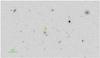 |
Fig. 1 Nordic Optical Telescope R-band image of the GB 1310+487 region obtained on 2011 May 29. The exposure time was 300 s. North is up and east is to the left. The AGN and comparison star SDSS J131240.83+482842.9 used in the NOT data analysis are marked with the letters “Q” and “C,” respectively. |
Kanata, a 1.5 m telescope at the Higashi-Hiroshima Observatory, observed GB 1310+487 in the R and I bands with the HOWPol instrument (Kawabata et al. 2008) in the nonpolarimetric mode for eight nights during the first and second γ-ray flares. Relative point-spread function (PSF) photometry was conducted using 3UC 277-116569 (αJ2000 = 13h12m54.s09,  , J2000; R = 16.109, I = 15.657 mag; Zacharias et al. 2010) as the comparison star. The adopted Galactic extinction values were AR = 0.035 and AI = 0.025 mag (Schlegel et al. 1998). The calibration by Bessell et al. (1998) was employed for the magnitude-to-flux conversion.
The source GB 1310+487 was assigned a redshift of 0.501 based on a 2007 March 21 1200 s Hobby-Eberly Telescope Low Resolution Spectrograph (HET/LRS) observation10, which showed strong [O II] λ3727 at 5592 Å and weak evidence of host absorption features (Healey et al. 2008; Shaw et al. 2012). This spectrum had insufficient S/N to exclude weak broad lines, or to cleanly measure the optical continuum, leaving the nature of the source uncertain.
Thus, we reobserved the source with the Keck 10 m telescopes. Long-slit spectra were obtained with the Keck II DEep Imaging Multi-Object Spectrograph (DEIMOS; Faber et al. 2003) on 2013 April 07 with ~ 1′′ seeing. Two 600 s integrations were obtained using the 600 lines per mm (7500 Å blaze11) grating, providing coverage in the 4450–9635 Å range with a ~ 100 Å gap between the two CCDs. With the  slit, the spectra have an effective resolution of ~ 3.0 Å. Conditions were good, but not completely photometric; the flux scale might be uncertain by roughly a factor of 2. Moreover, we obtained 2 × 180 s g- and R-band images of the object with the two cameras on the Keck I Low Resolution Imaging Spectrometer (LRIS; Oke et al. 1995) on May 10 under ~ 1′′ seeing, as shown in Fig. 2. The DEIMOS slit on April 07 was placed on the bright core of the source, at the parallactic angle (Filippenko 1982) of PA = 143° (measured from N to E), and the extended wings of the host were also included. The companion was ~ 3′′ off the slit.
A second Keck II/DEIMOS spectrum was obtained on June 10 with a different slit position and ~ 0.7′′ seeing. It has a higher S/N than the first DEIMOS spectrum; however, it was affected by a cosmic-ray hit that prevented accurate measurement of Hγ in the z = 0.638 system, and conditions were not photometric when the standard star was being observed. The two spectra are normalized to epoch 1 (April 07) using the [O II] λ3727 line at z = 0.500. The continuum cannot be used to cross-calibrate the two spectra because of the significantly variable AGN flux contribution; the second-epoch continuum level appears to have dropped relative to the emission lines by ~ 1/3. The two spectra were averaged for further analysis.
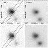 |
Fig. 2 Keck I/LRIS images of GB 1310+487 obtained on 2013 May 10. Top panel: the g- and R-band images (8′′ × 8′′ field of view; north is up and east is to the left). Bottom panel: g- and R-band images after subtraction of a scaled point source from the offset core. The boxes show the location of the DEIMOS slit in the 2013 April 07 observations. The circles indicate the location of the radio-loud AGN. These residual images reveal a relatively undisturbed foreground galaxy. |
2.5. Infrared photometry
Observations in the near-IR were carried out with the 2.1 m telescope of the Guillermo Haro Observatory, INAOE, Mexico. The telescope is equipped with the CANICA camera together with J, H, and Ks filters. We carried out differential photometry between the object of interest and other objects in the 5′ × 5′ field. The observations showed an increase of about one magnitude during the Flare 2 period with respect to the Flare 1 and post-flare periods (results are summarized in Table 3). Magnitudes are referred to the 2MASS12 survey published photometry. The source GB 1310+487 itself was not detected in the 2MASS survey. The survey detection limit is J = 15.8, H = 15.1, and Ks = 14.3 mag (Skrutskie et al. 2006). These values may be considered upper limits on the object brightness at the 2MASS observation epoch of JD 2451248.8408 (1999 March 11).
The source GB 1310+487 is listed in the Wide-field Infrared Survey Explorer (WISE; Wright et al. 2010) catalogue (Cutri et al. 2012) with the following magnitudes in the four WISE bands: 3.4 μm W1 = 12.302 ± 0.024, 4.6 μm W2 = 11.254 ± 0.021, 12 μm W3 = 8.596 ± 0.021, and 22 μm W4 = 6.368 ± 0.044. The IR colors (W1–W2 = 1.048 ± 0.032, W2–W3 = 2.658 ± 0.030 mag) are at the blue edge of the area in the color–color diagram occupied by blazars and Seyfert galaxies (see Fig. 12 in Wright et al. 2010; Fig. 1 in D’Abrusco et al. 2012; and Fig. 1 in Massaro et al. 2011), indicating that the AGN and not the host galaxy’s stars or warm dust is responsible for most of the IR flux in these bands. WISE observations of this area were conducted on 2010 June 3–8 during Flare 2 (Table 1).
Ground-based photometry of GB 1310+487.
2.6. Radio observations
As part of an ongoing blazar monitoring program, the Owens Valley Radio Observatory (OVRO) 40 m radio telescope has observed GB 1310+487 at 15 GHz regularly since the end of 2007 (Richards et al. 2011). This monitoring program studies over 1500 known and likely γ-ray-loud blazars, including all CGRaBS (Healey et al. 2008) sources north of declination −20°. The objects in this program are observed in total intensity twice per week. The minimum measurement uncertainty is 4 mJy while the typical uncertainty is 3% of the measured flux. Observations are performed with a dual-beam (each 2.5 full width at half-maximum intensity, FWHM) Dicke-switched system using cold sky in the off-source beam as the reference. Additionally, the source is switched between beams to reduce atmospheric variations. The absolute flux-density scale is calibrated using observations of 3C 286, adopting the flux density (3.44 Jy) from Baars et al. (1977). This results in a ~ 5% absolute flux-density-scale uncertainty, which is not reflected in the plotted errors.
Multifrequency radio observations of GB 1310+487 were performed with the 100 m Effelsberg telescope operated by the MPIfR13. Observations were conducted on 2009 December 1 following the reported γ-ray flare, on 2010 June 28 during the second γ-ray active phase, and on 2011 June 5. Secondary focus heterodyne receivers operating at 2.64, 4.85, 8.35, 10.45, and 14.60 GHz were used. The observations were conducted with cross-scans (i.e., the telescope’s response was measured while slewing over the source position in azimuth and elevation). The measurements were corrected for (a) pointing offsets; (b) atmospheric opacity; and (c) elevation-dependent gain (see Fuhrmann et al. 2008; Angelakis et al. 2009). The multifrequency observations were completed within 1 hr for each observing session. The absolute flux-density calibration was done by observing standard calibrators such as, 3C 48, 3C 161, 3C 286, 3C 295, and NGC 7027 (Baars et al. 1977; Ott et al. 1994).
The IRAM 30 m Pico Veleta telescope observations at 86.24 and 142.33 GHz took place on 2009 December 7. The observations and data-reduction strategy were similar to those with Effelsberg; a detailed description is given by Nestoras et al. (in prep.). Both the Effelsberg 100 m and IRAM 30 m telescope observations were conducted in the framework of the F-GAMMA program (Fuhrmann et al. 2007, and in prep.; Angelakis et al. 2008, 2010, 2012).
For comparison with the latest Effelsberg, IRAM, and OVRO results, we use data from the RATAN-600 576 m ring radio telescope of the Special Astrophysical Observatory (Russian Academy of Sciences); RATAN-600 observations of GB 1310+487 were performed in transit mode at the southern sector with the flat reflector quasi-simultaneously at 3.9, 7.7, 11.1, and 21.7 GHz in June 2003 within the framework of the spectral survey conducted by Kovalev et al. (1999b, 2002). The flux-density scale is set using calibrators listed by Baars et al. (1977); Ott et al. (1994). Details on the RATAN-600 observations and data processing are discussed by Kovalev et al. (1999a).
The National Radio Astronomy Observatory’s Very Long Baseline Array (VLBA, Napier 1994, 1995) is a system of ten 25 m radio telescopes dedicated to very long baseline interferometry (VLBI) observations for astrophysics, astrometry, and geodesy. After publication of the report on the November 2009 γ-ray flare (Sokolovsky et al. 2009), GB 1310+487 was added to the MOJAVE14 program (Lister et al. 2009a). Three epochs of VLBA observations at 15 GHz were obtained between 2009 and 2010.
3. Results
3.1. γ-ray analysis
The γ-ray counterpart of GB 1310+487 was localized, integrating 33 months of Fermi/LAT monitoring data, to αJ2000 = 198.°187, δJ2000 = 48.°472, with a 68% uncertainty of 0.°014 = 50′′. This is a factor of five larger than the spacecraft alignment accuracy of 10′′ = 0.°003 (Nolan et al. 2012). The γ-ray position is only 0.°005 = 18′′ away from the radio position of GB 1310+487. Within the Fermi/LAT error circle no other radio sources are seen with the VLA FIRST 1.4 GHz survey (White et al. 1997), which provides the best combination of sensitivity and angular resolution for that region of the radio sky to date. Therefore, the positional association of the γ-ray source with the radio source GB 1310+487 is firmly established. The X-ray brightening observed during the first and, to a lesser extent, the second γ-ray flares together with the near-IR brightening during the second γ-ray flare support the identification of the γ-ray source with the lower-frequency counterpart. See Tables 1, 2, 3, and the discussion below for details.
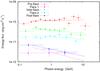 |
Fig. 3 Fermi/LAT γ-ray SEDs compared to the power-law models (shown as lines in this logarithmic plot) derived from unbinned likelihood analysis. We stress that the power-law models are not fits to the binned energy flux values; rather, these are two independent ways to represent Fermi/LAT photon data. The time intervals defined in Table 1 are color labeled. |
The γ-ray spectra of GB 1310+487 at various activity states listed in Table 1 are presented in Fig. 3. The plotted spectral bins satisfy the following requirements: TS > 50 and/or model-predicted number of source photons N> 8. The flux value at each bin was computed by fitting the model with source position and power-law photon index fixed to the values estimated over the entire period in the 0.1–100 GeV energy range. The Galactic component parameters were fixed, as were all other nontarget source components of the model.
To test if the power law (PL) is an adequate approximation of the observed γ-ray spectrum, the PL fit (represented by a straight line if plotted on a logarithmic scale) was compared to the fit with a log-parabola (LP) function defined as dN/ dE = N0(E/E0)− (α + βln(E/E0)), where N is the number of photons with energy E, N0 is the normalization coefficient, E0 is a reference energy, α is the spectral slope at energy E0, and β is the curvature parameter around the peak. For the combined 33 month Fermi/LAT dataset, the fit with the assumption of a PL spectrum for the target source provides its detection with the Test Statistic TSPL = 4415, while the LP spectrum leads to TSLP = 4423. These values may be compared by defining, following Nolan et al. (2012) and in analogy with the source detection TS described in Sect. 2.1, the curvature Test Statistic TScurve ≡ 2(lnLLP − lnLPL) = TSLP − TSPL. The obtained value of TScurve = 8 corresponds to a 2.8σ difference, which is lower than the TScurve> 16 (4σ) threshold applied by Nolan et al. (2012). We conclude that while there is a hint of spectral curvature, it cannot be considered significant.
The broken power-law (BPL) model was also tested, but it did not provide a statistically significant improvement over the PL or the LP models (TSBPL = 4423, for the best-fit break energy Eb = 3 GeV, the photon indexes Γph 1 = 2.30 ± 0.04, Γph 1 = 0.05 ± 0.02 above and below the break, respectively). Therefore, we adopt the simpler PL model for the following analysis.
The 33-month γ-ray lightcurve of the source obtained with the seven-day binning is presented in Fig. 4. Two major flaring periods are clearly visible. The first, brighter flare peaked around 2009 November 27 (JD 2 455 163) with the weekly averaged flux of (1.4 ± 0.1) × 10-6 photons cm-2 s-1. The peak flux averaged over the two-day interval centered on that date is (1.9 ± 0.2) × 10-6 photons cm-2 s-1. The source continued to be observed at a daily flux of ~ 0.5 × 10⁻⁶ photons cm-2 s-1 for another two weeks. The second flare peaked around 2010 June 17 (JD 2 455 365) at the seven-day integrated flux of (0.54 ± 0.07) × 10-6 photons cm-2 s-1. The daily flux of ~ 0.5 × 10⁻⁶ photons cm-2 s-1 was observed for about three weeks around this date. The two flares demonstrate remarkably contrasting flux evolution: the first is characterized by a fast rise and slower decay, while the second flare shows a gradual flux rise followed by a sharp decay. Following Burbidge et al. (1974), Valtaoja et al. (1999), and Gorshkov et al. (2008), we define the flux-variability timescale as tvar ≡ Δt/ ΔlnS, where ΔlnS is the difference in logarithm of the photon flux at two epochs separated by the time interval Δt. The observed flux-variability timescale during the onset of Flare 1, as estimated from the seven-day binned lightcurve (Fig. 4), is tvar ≈ 3 days. The timescale of flux decay after Flare 2 is tvar ≈ 5 days.
The Fermi/LAT lightcurve constructed with the alternative analysis method, the adaptive binning (with 25% flux uncertainty at each bin), is presented in Fig. 5. It confirms all the features visible in the constant bin-width lightcurve, but also allows us to investigate fast variability during high-flux states in greater detail. The first flare episode, Flare 1, consists of four prominent subflares, each with a time width of a day or less. The subflares show no obvious asymmetry and the variability timescale tvar for the three point rise of the second and third subflares (at JD 2 455 157.5 and 2 455 161.5) was estimated as 0.36 ± 0.20 days and 0.45 ± 0.23 days, respectively. A second adaptively binned lightcurve was produced in the reverse-time direction, which gives a similar, but not identical, time binning. The result of the timescale estimates for this second version of the lightcurve was found to be consistent with the first analysis. A similar analysis for the lightcurves with 15% uncertainties give timescale estimates of about 1 day for the most rapid variability. We conclude that the adaptively binned lightcurves show evidence of a variability timescale of half a day with a conservative upper limit of 1 day. For the second and fainter flare epoch the timescales seen in the adaptive binning are consistent with the estimate from the fixed-binned lightcurve described above.
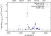 |
Fig. 4 Weekly binned Fermi/LAT lightcurve. Blue filled circles are values with TS > 25, gray filled circles are values with 5 < TS < 25, and gray arrows indicate 2σ upper limits for time bins with no significant detections (TS < 5). A four-day integrated AGILE data point is added as an open box for comparison. |
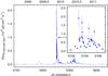 |
Fig. 5 Fermi/LAT lightcurve constructed with the adaptive binning method (Lott et al. 2012). The magnified plot of Flare 1 is shown in the insert. The energy range for this lightcurve is chosen to minimize the uncertainties in time and flux, while the lightcurve was Fig. 4 is given in the commonly used E> 100 MeV energy range. |
Table 1 presents spectral analysis results for the different γ-ray activity states of the source: “pre-flare” and “post-flare” periods represent the low-activity level, “Flare 1” and “Flare 2” represent the high-activity state, while during the “interflare” interval the source showed an intermediate γ-ray flux level. Figure 3 presents the observed Fermi/LAT spectrum during these states. Significant evolution of the γ-ray photon index, Γph, is detected between the different flux states (Table 1). Figure 6 presents Γph as a function of (E> 100 MeV) flux. The harder-when-brighter trend is clearly visible.
Integrating the AGILE observations from 2009 November 18 12:00 (JD 2 455 154.0) to 2009 November 22 12:00 UT (JD 2 455 158.0), we obtain a γ-ray flux FE> 100 MeV = (1.65 ± 0.48) × 10-6 photons cm-2 s-1, at a significance of  . This result is in good agreement with the flux value derived from the preliminary analysis by Bulgarelli et al. (2009). Prior to the Fermi launch, AGILE observed GB 1310+487(in pointing mode) during two other periods, but did not detect the source. During the first period (from 2007 October 24 12:00 UT to 2007 November 1 12:00 UT, JD 2 454 398.0–2 454 406.0), the 2σ upper limit was FE> 100 MeV ≤ 0.28 × 10⁻⁶ photons cm-2 s-1, while in the second period (from 2008 April 30 12:00 UT to 2008 May 10 12:00 UT, JD 2 454 587.0–2 454 597.0) we obtained a 2σ upper limit of FE> 100 MeV ≤ 0.31 × 10⁻⁶ photons cm-2 s-1.
3.2. X-ray to infrared spectrum
Results of the X-ray spectral analysis are presented in Table 2. The obtained values of the X-ray photon index Γph X - ray are among the hardest reported for blazars (Giommi et al. 2002; Donato et al. 2005; Sikora et al. 2009). Radio-loud NLSy1 have Γph X - ray similar to the ones found in blazars (Paliya et al. 2013; Abdo et al. 2009d). However, it cannot be excluded that the X-ray spectrum with an intrinsic value of Γph X - ray is artificially hardened by additional absorbing material along the line of sight (see the discussion of NOT imaging results below). Future high-quality X-ray observations are necessary for investigating this possibility.
The UV and blue parts of the optical spectrum are flat, in contrast to the steep spectrum seen in the near-IR (iJHK bands). Also, the observed variability amplitude is decreasing toward bluer wavelengths, with the U-band brightness being essentially constant.
The H-band flux showed an increase of about one magnitude during the Flare 2 period with respect to the Flare 1 and post-flare periods, in contrast to the behavior seen in other bands. The results of ground-based photometric measurements are summarized in Table 3.
3.3. Imaging with NOT
The Nordic Optical Telescope images (Fig. 1) show a fuzzy extended object, probably a galaxy, with a point source offset  from its center. Considering that there are many galaxies of comparable brightness visible in the field, this picture may be interpreted as the AGN (corresponding to the point source) shining through an unrelated foreground galaxy. This may be the source of confusion in the AGN’s redshift determination (Sokolovsky et al. 2009; Healey et al. 2008; Falco et al. 1998), and it also explains the steepness of the optical-IR SED (the observed SED was corrected for Milky Way absorption, but absorption in the intervening galaxy may also be significant). On the other hand, it is not uncommon for AGN host galaxies to have disturbed morphologies, making it appear that the AGN is off-center.
The galaxy contributes a large fraction of the total optical flux, when the point source is in the low state. If the host galaxy of GB 1310+487 is similar to the giant ellipticals studied by Sbarufatti et al. (2005), ⟨ MR ⟩ = −22.9 ± 0.5 mag, its magnitude at z = 0.500 should be R ≈ 20 (or 0.6 mag fainter at z = 0.638; Sect. 3.4). A typical NLSy1 from the Véron-Cetty & Véron (2010) catalogue having ⟨ MV ⟩ = −21.4 mag would appear 1 mag fainter than a giant elliptical in the R band assuming V − R = 0.5 mag (Xanthopoulos 1996). Therefore, the observed galaxy could be the host of GB 1310+487. The visible offset between the point source and the center of extended emission could result from the disturbed morphology of the host, as noted above.
3.4. Keck imaging and spectroscopy
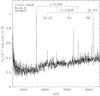 |
Fig. 7 Keck II/DEIMOS spectrum of GB 1310+487. The two narrow-line systems are indicated. The region 6900–7000 Å is lost to a gap between the two CCDs. The slit position is shown in Fig. 2. |
Standard reductions, extractions, and calibrations of the DEIMOS data produced the spectrum shown in Fig. 7; it is the average of two observations conducted on April 07 and June 10, 2013. The strongest line, [O II] λ3727, confirms the HET redshift identification at z = 0.500, and we also see [O III] and narrow Balmer emission for this system. However, there are additional lines, mostly in the red half. These represent a second system with narrow forbidden and Balmer emission, this time at z = 0.638. The line strengths are given in Table 4. The [O II] doublets are barely resolved, but the oxygen and Balmer line widths are consistent with the instrumental resolution. The [O III] emission at z = 0.638 appears resolved with a deconvolved width of ~ 200 km s-1. Unfortunately, the red limit of the spectrum does not include the Hα/[N II] lines for either system. For the z = 0.500 system, we cover [O I] λ6300, which is weak or absent. For the z = 0.638 system, we cover Mg II λ2800, and can place a 3σ rest equivalent width limit of ~ 1.0 Å on any broad emission; the Hβ line is marginally detected for the z = 0.638 system at 4σ level. The ratio of Hβ to [O III] (z = 0.638) is small, even if the Hβ flux is treated as an upper limit. Together with the resolved [O III] this indicates nuclear excitation.
GB 1310+487 emission-line strengths.
Multifrequency radio observations of GB 1310+487.
Thus, we clearly have two superimposed systems and wish to identify which system hosts the radio-loud core (and, by inference, the γ-ray source). The Keck I LRIS images confirm the basic structure seen in the NOT images; the source is extended with a brighter core displaced  to the west. Figure 2 shows 8′′ regions around the AGN. The DEIMOS slit position on April 07 is marked on the g frames (left). At the bottom we show the images after removal of a point-source PSF (g = 23.89, R = 22.45 mag) from the offset core. The residuals show a relatively regular galaxy having FWHM =
  , with g = 21.95 and R = 20.59 mag. The coordinate system was referenced through the SDSS image of the field, with an estimated uncertainty relative to the radio frame of
  ; the circles show the position of the VLBI source (Sect. 1) and have radii twice this uncertainty. Hence, the radio source is coincident with the point-like peak of the combined source. We also find that the z = 0.500 emission lines are offset
  SE along the slit from the z = 0.638 system, toward the continuum tail representing the extended galaxy. The deprojected offset is
  E of the AGN core. We thus conclude that the true AGN redshift is z = 0.638, and we are viewing it through an approximately face-on galaxy showing strong narrow-line emission.
Our extracted spectrum is weighted toward the AGN core, although it also contains appreciable light from the foreground galaxy. Both spectra are dominated by narrow forbidden lines, yet there is appreciable continuum associated with both components as well. The foreground galaxy is probably not an AGN, but we cannot be certain; without the [N II]/Hα line ratio, we are unable to fully distinguish “LINER” (Low Ionization Nuclear Emission-line Region) emission from an H II region (e.g., Ho et al. 1997). However, the strong [O II] λ3727 and lack of obvious [O I] λ6300 argue against a power-law ionizing spectrum, suggesting that the z = 0.500 emission represents star formation in the foreground galaxy lacking AGN activity.
The positional accuracy of the available observations of multiwavelength variability (Sect. 2) is not sufficient to distinguish between the foreground and background objects discussed here and in Sect. 3.3 as the source of high-energy emission. The proposed interpretation that the background AGN is the high-energy source rests on the consideration that the observed fast γ-ray variability (Sect. 3.1) is typical of radio-loud AGNs (which the background source is), while there are no firm indications of AGN activity in the foreground galaxy.
3.5. Results of radio observations
The radio spectrum of GB 1310+487 is generally flat, with a wide peak located between 22 GHz and 86 GHz (Table 5). The variability amplitude at 2.64 GHz is slightly lower compared to higher frequencies. The 15 GHz lightcurve of GB 1310+487 obtained with the OVRO 40 m telescope and complemented by measurements with the Effelsberg 100 m and the VLBA is presented in Fig. 8. It shows a period of high activity with two separate peaks that started in mid-2010 and is still ongoing.
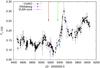 |
Fig. 8 Radio lightcurve at 15 GHz obtained with the OVRO 40 m telescope (points) supplemented with two 14.6 GHz measurements obtained with the Effelsberg 100 m telescope (square). VLBA measurements of the core (component C0, Table 6) are indicated as diamonds. The two arrows mark the peaks of the γ-ray flares observed by Fermi. |
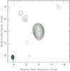 |
Fig. 9 VLBA radio image of GB 1310+487 obtained on 2010-12-24 at 15 GHz during the course of the MOJAVE program. The image map peak is 0.206 Jy beam-1 and the first contour is 0.15 mJy beam-1. Adjacent contour levels are separated by a factor of 2. Naturally weighted beam size is indicated at the lower-left corner of the image. Green circles indicate positions and best-fit sizes of the model components presented in Table 6. |
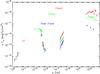 |
Fig. 10 Quasi-simultaneous radio to γ-ray SED of GB 1310+487 during the two flaring episodes and the post-flare period covered by our multiwavelength observations. The time intervals corresponding to these events are defined in Table 1. |
Parsec-scale components observed at 15 GHz.
The 15 GHz VLBA images (Fig. 9) show two emission regions separated by ~ 0.4 mas. To quantify their parameters we fit the observed visibilities with a model consisting of two circular Gaussian components using the Difmap software (Shepherd 1997). The modeling results are presented in Table 6. The uncertainties in parameters of the model components were estimated following Lee et al. (2008), and the resolution limit achieved for each component was computed following Lobanov (2005) and Kovalev et al. (2005).
The SW component increased its brightness during the three epochs. Comparison with the lightcurve in Fig. 8 shows that this component is responsible for most of the flux observed with single-dish instruments. The fainter component located to the NE is gradually fading. If the SW component is the 15 GHz core, the position of the second component aligns nicely with the orientation of the kiloparsec-scale jet observed with the VLA at 1.4 GHz by Machalski & Condon (1983). No significant proper motion could be detected between the three 15 GHz MOJAVE epochs. The 3σ upper limit which can be placed on proper motion is μ< 0.3 mas yr-1, corresponding to βapp< 11 (βapp is in units of the speed of light) at the source redshift, which is within the range of apparent jet speeds occupied by γ-ray-bright blazars (Lister et al. 2009b; Savolainen et al. 2010). The projected linear size of the double structure resolved with the VLBA is ~ 2.7 pc = 8 × 1018 cm. The overall 15 GHz VLBI polarization of the source measured by MOJAVE is 2.8–6.5% which is indicative of beamed blazar emission. The weakly beamed, high viewing angle sources in MOJAVE tend to be unpolarized (Lister & Homan 2005).
3.6. SED during the two flares
The SED of GB 1310+487 is presented in Fig. 10. It has the classical two-humped shape with the high-energy hump dominating over the synchrotron hump during the first (brighter) flare by a Compton dominance factor of q ≥ 10. For the Flare 2 period the value of Compton dominance may be measured accurately thanks to simultaneous observations of Fermi/LAT and WISE: q = 12. The uncertainty of this measurement is limited by the accuracy of the absolute calibration of the two instruments and should be less than 10%. Fast variability within the Flare 2 period may also contribute to the uncertainty. The value of q is probably larger for Flare 1 than for Flare 2, judging from the lower near-IR flux observed during Flare 1.
4. Discussion
4.1. γ-ray luminosity, variability, and spectrum
The monochromatic γ-ray energy flux averaged over the duration of the first flare is νFν ≈ 10-10 erg cm-2 s-1. At the redshift of the source this corresponds to an isotropic luminosity of ~ 1047 erg s-1. Considering the expected bolometric correction of a factor of a few, the γ-ray luminosity of GB 1310+487 is comparable to that typically observed in flaring γ-ray blazars (e.g., Tanaka et al. 2011; Abdo et al. 2010a,e) and NLSy1 (D’Ammando et al. 2013). It is about two orders of magnitude lower than the most extreme GeV flares of 3C 454.3 in November 2010 (Abdo et al. 2011b) and PKS 1622–297 in June 1995 (Mattox et al. 1997). The outstanding γ-ray flare of 3C 120 in November 1968 had a comparable isotropic luminosity of ~ 1047 erg s-1 (Volobuev et al. 1972). The exceptional GeV photon flux of 3C 120 was due to the relative proximity of the source (z = 0.033; Michel & Huchra 1988) compared to the brightest γ-ray blazars mentioned above. The observed large γ-ray luminosity of GB 1310+487 is an indirect indication of a high Doppler boosting factor of the source (Taylor et al. 2007; Pushkarev et al. 2009).
The difference in lightcurve shape, overall duration, and shortest observed variability timescale between the two flares of the source may indicate that they occurred in different jet regions or were powered by different emission mechanisms as discussed below. In both cases, this implies differences in the emitting-plasma parameters for the two flares, such as the electron energy distribution, magnetic field strength, bulk Lorentz factor, or external photon field strength. Variability timescales of 3 days and shorter are common in GeV blazars (e.g., Mattox et al. 1997; Abdo et al. 2010f, 2011b; Sbarrato et al. 2011). The light-travel-time argument limits the γ-ray emitting region size r<cδtvar/ (1 + z) ≈ a few × 1015 cm, where c is the speed of light in vacuum, z is the source redshift, and conservatively assuming the Doppler factor δ ≡ [Γ(1 − βcosθ)] -1< a few (we have no evidence of extreme Doppler boosting from VLBI and γ-ray data; Sect. 4.2), where Γ is the Lorentz factor, β is the bulk velocity of the emitting blob in units of the speed of light, and θ is the angle between the blob velocity and the line of sight.
It is important to check that the observed harder-when-brighter trend in the γ-ray spectrum is not related to the expected correlation between the flux and the index in the power–law model. If the number density of photons arriving from the source is dN/ dE = N0(E/E0)− Γph (where N0, and E0 are constants), the integrated photon flux between energies Emax and Emin is ![Mathematical equation: \begin{eqnarray*} F = \frac{N_0 E_0}{-\Gamma_\mathrm{ph}+1} \left[\left(\frac{E_\mathrm{max}}{E_0}\right)^{-\Gamma_\mathrm{ph}+1} - \left(\frac{E_\mathrm{min}}{E_0}\right)^{-\Gamma_\mathrm{ph}+1} \right]. \end{eqnarray*}](/articles/aa/full_html/2014/05/aa20703-12/aa20703-12-eq284.png) Assuming that Γ > 1 and Emax is large,
Assuming that Γ > 1 and Emax is large, 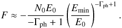 The derivative
 ![Mathematical equation: \begin{eqnarray*} \frac{\mathrm{d}F}{\mathrm{d}\Gamma_\mathrm{ph}} = F \left[\frac{1}{-\Gamma_\mathrm{ph}+1} - \ln\left(\frac{E_\mathrm{min}}{E_0}\right) \right] \neq 0 \end{eqnarray*}](/articles/aa/full_html/2014/05/aa20703-12/aa20703-12-eq287.png) if ln(Emin/E0) ≠ 1/( − Γph + 1). The range of parameters derived from our analysis is Γ = 1.97–2.41, Emin = 100 MeV, E0 = 283 MeV, and −1.04 = ln(Emin/E0) < 1/( − Γph + 1) = −1.03 to −0.70, so dF/ dΓph> 0. The expected correlation between dF and Γph due to their mathematical dependence is positive, which is opposite to what is actually observed. We conclude that the observed harder-when-brighter trend is real and not related to the intrinsic correlation of the model parameters.
if ln(Emin/E0) ≠ 1/( − Γph + 1). The range of parameters derived from our analysis is Γ = 1.97–2.41, Emin = 100 MeV, E0 = 283 MeV, and −1.04 = ln(Emin/E0) < 1/( − Γph + 1) = −1.03 to −0.70, so dF/ dΓph> 0. The expected correlation between dF and Γph due to their mathematical dependence is positive, which is opposite to what is actually observed. We conclude that the observed harder-when-brighter trend is real and not related to the intrinsic correlation of the model parameters.
Previously a harder-when-brighter trend (Fig. 6) has been seen at GeV energies only in a handful of blazars: 3C 273, PKS 1502+106, AO 0235+164, and 4C +21.35 by Fermi (Abdo et al. 2010k,f,g; Tanaka et al. 2011); 3C 454.3 (Ackermann et al. 2010; Vercellone et al. 2010; Abdo et al. 2011b; Stern & Poutanen 2011) and PKS 1510−089 by Fermi and AGILE (Abdo et al. 2010a; D’Ammando et al. 2011); and 3C 279 (Hartman et al. 2001) and PKS 0528+134 (Mukherjee et al. 1996) by EGRET. The same harder-when-brighter behavior was suggested by the combined analysis of relative spectral index change as a function of relative flux change in a few of the brightest FSRQs, low-, and intermediate-peaked BL Lacs using the first six months of Fermi data by Abdo et al. (2010g). The current detection presents one of the clearest examples of this spectral behavior.
The spectral evolution during the Flare 1–interflare–Flare 2 periods (Fig. 3 and Table 1) may be qualitatively understood as the gradual decrease in energy of the γ-ray emission peak. During Flare 1, the spectrum is hard, implying that the spectral peak is located above or around 5 GeV. Consequently, during the interflare period the spectrum is softer, with a hint of curvature; the emission peak may be located around 1–2 GeV. Later, during Flare 2, the spectrum is also soft with a peak possibly located at even lower energies. This interpretation is inspired by the visual inspection of Fig. 3. The peak-frequency evolution is difficult to quantify owing to the insufficient number of collected photons, which results in the simple PL fit (with no curvature) being a statistically acceptable model for the LAT data. However, the overall SED (Fig. 10) suggests that the high-energy emission peak should be located somewhere around the LAT band. We can use the LAT spectral index (Γph) vs. Compton peak frequency ( ) correlation
 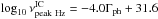 reported by Abdo et al. (2010b) to estimate that changed from 1022 to 1024 Hz between the pre-flare and Flare 1 periods. The change in may result not from a continuous shift of a single γ-ray emission peak, but from a change in relative strengths of two emission components peaking at different frequencies, as discussed in Sect. 4.9.
4.2. Jet Doppler factor
The Doppler factor of the relativistic jet in GB 1310+487 may be constrained using two independent lines of argument: one based on the requirement that the emitting region should be transparent to its own γ radiation (since we observe it), the other based on the absence of apparent proper motion seen by the VLBA.
The minimum Doppler factor needed to avoid γ − γ attenuation for γ-rays interacting with lower energy photons present inside the emitting region may be calculated using Eq. (39) of Finke et al. (2008), ![Mathematical equation: \begin{eqnarray*} \delta_{\gamma\gamma} > \left[\frac{ 2^{a-1} (1+z)^{2-2a} \sigma_T D_L^2} {m_{\rm e} c^4 t_\mathrm{var} } \epsilon_1 f_{\epsilon_1^{-1}}^{\rm syn} \right]^{\frac{1}{6-2a}}, \end{eqnarray*}](/articles/aa/full_html/2014/05/aa20703-12/aa20703-12-eq303.png) where it is assumed that the synchrotron flux is well represented by a power law of index a (
where it is assumed that the synchrotron flux is well represented by a power law of index a ( ), σT is the scattering Thomson cross-section, DL is the luminosity distance to the source, me is the electron mass, and ϵ1 = E/ (mec2) is the dimensionless energy of a γ-ray photon with energy E for which the optical depth of the emitting region τγγ = 1 (see also Dondi & Ghisellini 1995). The maximum energy of observed γ-ray photons that can be attributed to the source is ~ 10 GeV (Fig. 3), so ϵ1 = 10 GeV/(5.11 × 10-4) GeV = 2 × 10⁴. This means
  , and the corresponding frequency for this is 6.3 × 10¹⁵ Hz. From the observed SED (Fig. 10), we estimate
  and a ≈ − 2. Taking tvar = 3 days (Sect. 3.1) we obtain δγγ> 1.5.
Assuming the angle between the jet axis and the line of sight, θ, is θmax, the one that maximizes the apparent speed, βapp, for a given intrinsic velocity, β, we may estimate the corresponding Doppler factor δVLBA< 11 (if  ). We note that if θ is smaller than θmax, the actual δ will be larger than the above estimate (see, e.g., Cohen et al. 2007; Kellermann et al. 2007; Marscher 2009 for a discussion of relativistic kinematics in application to VLBI).
Recent RadioAstron (Kardashev et al. 2013) Space–VLBI observations of high brightness temperatures in AGNs suggest that the actual jet flow speed is often higher than the jet pattern speed (Sokolovsky 2013). These results question the applicability of δ estimates based on VLBI kinematics. The available lower limits on the core brightness temperature, Tb, in GB 1310+487 (Table 6) are consistent with negligible Doppler boosting within the standard assumption of the equipartition inverse-Compton limited Tb ≈ a few × 1011 K (Readhead 1994).
4.3. Black hole mass
If we equate the linear size estimated from the shortest observed variability timescale to the Schwarzschild radius, the corresponding black hole mass would be M• ≈ 1010M⊙. However, TeV observations of ultra-fast (timescale of minutes) variability in blazars PKS 2155−304 (Aharonian et al. 2007; Abramowski et al. 2010) and Mrk 501 (Albert et al. 2007) lead to M• estimates inconsistent with those obtained by other methods (Begelman et al. 2008), unless an extremely large Doppler factor δ ≈ 100 is assumed for the γ-ray emitting region (Ghisellini & Tavecchio 2008; Sbarrato et al. 2011). Short timescale variability may arise from the interaction of small (size r<rs) objects such as stars (Barkov et al. 2012) or BLR clouds (Araudo et al. 2010) with a broad relativistic jet. This should caution us against putting much trust in the above M• estimate.
4.4. UV, optical, and IR emission
The UV-to-IR behavior of the source may be understood if the near-IR light is dominated by the synchrotron radiation of the relativistic jet, while in the optical–UV the contribution of line emission and/or thermal emission from the accretion disk starts to dominate over the synchrotron radiation. The line and thermal emission are not relativistically beamed and, therefore, more stable compared to the beamed synchrotron jet emission, decreasing the variability amplitude in the parts of the SED where their contribution to the total light is comparable to that from the jet. Thermal emission features are observed in SEDs of many FSRQ-type blazars (e.g., Villata et al. 2006; Hagen-Thorn et al. 2009; Abdo et al. 2010a; D’Ammando et al. 2011). Starlight from the host galaxy also contributes to the total optical flux in some γ-ray loud AGN (Nilsson et al. 2007; Abdo et al. 2011a,c). This contribution is significant mostly for BL Lac-type blazars and non-blazar AGN. Finally, as discussed above, the nearby galaxy and the star-like object, both probably unrelated to the source under investigation, may contribute to its total optical flux if an observation lacks angular resolution to separate contributions from these objects.
4.5. Radio properties
The radio loudness parameter, Rradio, defined as the ratio of 5 GHz flux density, L5 GHz, to the B-band optical flux density, LB, is Rradio = L5 GHz/LB ≈ 104. This is an order of magnitude larger than typical Rradio values found in quasars (Kellermann et al. 1989) and radio-loud NLSy1 galaxies (Doi et al. 2006), but it is comparable to the largest observed values (Singal et al. 2013)15. The extremely low optical luminosity compared to the radio luminosity may either be an intrinsic property of this source, or it may result from absorption in the intervening galaxy (Sects. 3.3, 3.4).
The radio spectrum of GB 1310+487 (Table 5) is typical for a blazar. Relatively rapid (timescale of months) and coherent changes across the cm band suggest that most of the observed radio emission comes from a compact region no more than a few parsecs in size. Comparison of the 15 GHz lightcurve presented in Fig. 8 with the 15 GHz VLBA results (Table 6) indicates that the component C0 (presumably the core) is the one responsible for most of the observed single-dish flux density of the source. Specifically, C0 is the site of the major radio flare peaking around JD 2 455 500 (October–November 2010).
The presence of correlation between cm-band radio and γ-ray emission is firmly established for large samples of blazars (Ackermann et al. 2011; Arshakian et al. 2012; Linford et al. 2012; Kovalev 2009). The typical γ-ray/radio time delay ranges from 1 month to 8 months in the observer’s frame, with γ-rays leading radio emission (Pushkarev et al. 2010; León-Tavares et al. 2011). However, for individual sources it is often difficult to establish a statistically significant correlation because of the limited time span of simultaneous γ-ray–radio data compared to a typical duration of radio flares (Max-Moerbeck et al. 2012). This could also limit our knowledge of the maximum possible radio/γ-ray time delay.
In the case of GB 1310+487, no clear connection is visible between its radio and γ-ray activity, based both on the available single-dish (Fig. 8) and VLBI monitoring data (Table 6).
4.6. Object classification
Shaw et al. (2012) classified the optical spectrum of GB 1310+487 as a LINER, which is inconsistent with the γ-ray and radio loudness (Sect. 4.5; Giuricin et al. 1988). The absence of broad lines precludes classification as a quasar. Prominent forbidden emission lines are not typical of BL Lac-type objects. Therefore, while being similar to blazars in its high-energy, radio, and IR properties, GB 1310+487 cannot be classified as a classical blazar on the basis of its optical spectrum.
As discussed in Sect. 3.4, the point-source emission at z = 0.638 observed by Keck is most likely related to the AGN. Pogge (2000) defines NLSy1 as having permitted lines only slightly stronger than forbidden lines, [O III]/Hβ< 3, and FWHM(Hβ) < 2000 km s-1. The anomalously strong [O III] λλ4959, 5007 emission formally disqualifies this source, and tends to support a Seyfert 2 (or a narrow-line radio galaxy, considering the object’s radio loudness) classification, which would be difficult to understand if the radio- and γ-ray jets align with the Earth’s line of sight. Our S/N is too low to allow unambiguous detection of Fe II emission. Broad Hβ, if present, is weaker than a third of the narrow component, and there is no evidence of Mg II 2800 Å. Thus, no broad-line component is observed. We also find that Ca H&K are weak, if present, and the 4000 Å break is smaller than 0.1. These aspects suggest appreciable nonthermal luminosity for the core AGN emission. Thus, we tentatively advance the view that synchrotron emission from the AGN dominates the variable point-source core, but that a surrounding narrow line region dominates the line flux.
Gurkan et al. (2014) studied the WISE infrared colors of radio-loud AGN; GB 1310+487 falls in a region of the color diagram occupied mostly by quasars and broad-line radio galaxies, although some narrow-line radio galaxies are also present. The source GB 1310+487 is well away from the locus of low-excitation radio galaxies (LERGs) and also has a 22 μm luminosity (~ 4 × 1045 erg s-1) typical of high-excitation radio galaxies (HERGs; see Fig. 8 in Gurkan et al. 2014). However, if one uses the criteria of Jackson & Rawlings (1997) GB 1310+487 would qualify as a LERG based on its optical spectrum. We note that WISE photometry of the AGN might be contaminated by the foreground galaxy.
Being a narrow-line radio-loud AGN, the object is not a member of common types of γ-ray flaring extragalactic sources (blazars and NLSy1s). One possibility is that the object is analogous to nearby radio galaxies like Per A with additional amplification due to gravitational lensing that makes γ-ray emission from its core detectable at high redshift. The similarity to Per A is supported by its lack of superluminal motion (Lister et al. 2013), low δ inferred from SED modeling (Abdo et al. 2010h), and absence of changes in VLBI and single-dish radio properties that can be attributed to GeV events (Nagai et al. 2012).
Another possibility is that the object may be a bona fide blazar with its optical non-thermal emission swamped by the host elliptical as proposed by Giommi et al. (2013) as possible counterparts of unassociated Fermi sources. In this case, however, one would not understand the observed variable optical point source. Higher S/N spectroscopy with increased wavelength coverage would be helpful in characterizing the z = 0.638γ-ray/radio AGN. Higher resolution spatial imaging is needed to probe the nature of the foreground (z = 0.500) galaxy.
4.7. Gravitational lensing
Considering that the AGN is located behind the visible disk of another galaxy (Sects. 3.4, 4.6), amplification of the AGN light by gravitational lensing is a real possibility. In the simplified case of a point lens, the AGN light is amplified by a factor of  (Paczynski 1986; Griest 1991; Wambsganss 2006), where u is the ratio of the AGN/lensing-galaxy separation () to the lensing galaxy’s Einstein radius,
  where G is the gravitational constant, M is the lensing galaxy mass, Dlens = 1300 Mpc is the angular size distance to the lens, DAGN = DA = 1400 Mpc is the angular size distance to the AGN, Dlens − to − AGN = DAGN − (1 + zlens)/(1 + zAGN)Dlens is the distance between the lens located at redshift zlens and the AGN located at redshift zAGN, and Mlens 12 is M expressed in the units of 1012M⊙. The above amplification factor estimate involves a number of simplifications including (i) the simplified lens geometry; (ii) use of the observed AGN–lens separation which is larger than the true one; and (iii) the Paczynski (1986) formula referring to the combined light of two images (we know from observations that the single observed image of GB 1310+487 is much brighter than its second undetected image). Taking into account these caveats, we estimate that the AGN image is probably amplified by a factor of a few.
Since no second image is visible in optical Keck and radio VLBA (this work) and VLA (JVAS survey; King et al. 1999) data, we assume that its contribution to the source lightcurve at other bands, including GeV, is also negligible. The absence of an observable second image may indicate that either the lens is not massive and the source is still outside its RE or the mass distribution in the lens is asymmetric and the lensed source is close to a fold or cusp caustic. If the lens is a singular isothermal sphere (SIS; e.g., Refsdal & Surdej 1994; Meylan et al. 2006) and the lensed AGN is just outside the Einstein radius defined for an SIS through the lensing galaxy’s velocity dispersion σSIS,  then a single image is formed having, in principle, an arbitrarily large amplification factor A = 1/(1 − 1 /u) (e.g., Wu 1994). Taking
  we estimate σSIS ≤ 140 km s-1 and the mass inside RE SIS of ≤6 × 10¹⁰M⊙ (Fort & Mellier 1994). The low lensing galaxy mass, necessary to put the AGN image outside RE (and form a single image), may be reconciled with its brightness if the galaxy is undergoing intensive star formation, as indicated by strong emission lines in its spectrum.
In general, gravitational lenses producing a single magnified image of a distant source should be more common than lenses producing multiple images. However, most gravitational lens searches (like the JVAS-CLASS survey; Browne et al. 2003) are designed to identify only multiple-image lenses. The BL Lac-type object AO 0235+164 is an example of a blazar shining through an intervening galaxy and having a single image weakly amplified by macrolensing (Abraham et al. 1993).
A possibility of microlensing by individual foreground stars in the z = 0.5 galaxy cannot be excluded. The timescale of such microlensing events may be estimated as a ratio of the Einstein radius for a single star to the proper motion of the lens and is on the order of tens of years. Therefore, microlensing is probably unrelated to the observed fast high-energy variability, but may provide a significant amplification that is nearly constant over the duration of our observations. A large constant amplification due to microlensing could also explain the absence of the second lensed image.
4.8. Emission model constraints from the SED
The high-energy SED hump dominates over the synchrotron hump during the first (brighter) flare by a factor of q> 10. This is commonly observed in FSRQ-type blazars. In the framework of the leptonic model, the large q suggests that most of the observed γ-ray flux during the first flare should be attributed to the EC process rather than to the SSC scenario. An SSC model would require a large deviation from equipartition: the emitting-particle energy density would need to be q2 times greater than the magnetic field energy density in the source frame (Sikora et al. 2009), which is not expected; EC models do not require deviation from equipartition to explain large values of q.
The dramatic difference in spectral slopes in the radio and IR regions suggests the presence of a break in the electron energy distribution. At the post-flare state, GB 1310+487 shows a steep γ-ray spectrum. If this spectrum is dominated by the SSC emission (Sect. 4.9), it is possible to estimate the Lorentz factor, γb, of electrons emitting at the energy distribution break from the positions of the SSC (νSSC ≈ 1022 Hz) and synchrotron (νsyn ≈ 1014 Hz) SED peaks (Sikora et al. 2009): γb ≈ (νSSC/νsyn)1/2 ≈ 104. This value is an order of magnitude larger than those found in detailed SED modeling of FSRQs, (e.g., Vercellone et al. 2011; Hayashida et al. 2012; Dutka et al. 2013). Different SED models applied to the same source may lead to different estimates of γb (Sokolovsky et al. 2010; Abdo et al. 2010a).
This is also the case for GB 1310+487 (Table 2). Hadronic models predict that X-rays are produced by synchrotron radiation of the secondary ultra-relativistic population of electrons and positrons. To reproduce the hard X-ray spectra observed in GB 1310+487 (Table 2) and in FSRQs, an extremely efficient acceleration of relativistic protons within the inner parts of the outflow is needed, and the jet kinetic power must be orders of magnitude larger than the Eddington luminosity (Sikora et al. 2009), making this scenario very unlikely.
4.9. Interpretation of changes in the SED
According to the leptonic interpretation of blazar SEDs outlined in Sect. 1, the near-IR flux should be dominated by the synchrotron radiation while the observed γ-ray flux is a combination of EC and SSC components. The lack of broad lines in the optical spectrum observed by us (Sect. 3.4) and Shaw et al. (2012) suggests that the BLR in GB 1310+487 is weak or obscured from view. This, however, does not exclude the EC scenario: photons from the accretion disk or dusty torus might serve as targets for inverse-Compton scattering. The optical–UV spectrum is flatter than the near IR one; however, due to contamination of the host (or intervening) galaxy and a nearby star (Sect. 3.3), it is not possible to distinguish accretion-disk emission that might be present in this wavelength range. It may also be that the accretion disk avoids detection because it emits at shorter wavelengths. This would be the case if the central black hole mass is smaller than the one typically found in blazars, since the accretion-disk temperature decreases with increasing M• (Shakura & Sunyaev 1973). Far-IR data available only during the high-IR state (Flare 2) are not sufficient to estimate the possible contribution from a dusty torus. Thus, accretion-disk and dusty torus luminosities remain as free parameters in this discussion.
The EC component peaks at higher energies than the SSC component for the following reasons. First, the typical energy of seed photons for the EC process (IR, optical, or UV corresponding to dusty torus, BLR, or accretion disk as the dominating source of external radiation) should be higher than the typical energy of synchrotron photons. The synchrotron emission peak is located in the far-IR, as suggested by the observed steep near-IR spectrum. Second, due to relativistic aberration, most external photons illuminate the synchrotron-emitting plasma blob head on. Therefore, the external photons are additionally blueshifted in the reference frame of the plasma blob. A change in relative strength of the EC and SSC humps may explain the observed γ-ray spectrum evolution, with the harder spectrum corresponding to greater contribution of the EC component to the total GeV flux. Large-amplitude GeV variability makes the corresponding spectral changes apparent even with the limited photon statistics of the observations.
Another way to explain the observed changes in the γ-ray spectrum is a varying contribution from multiple EC components (e.g., EC on accretion disk and dusty torus photons). This scenario, however, gives no predictions about the behavior of the synchrotron SED component, while the SSC+EC explanation is able to describe qualitatively the observed changes in the low-energy SED hump.
The difference in SED during Flare 1 and Flare 2 may be qualitatively understood if the two flaring events are triggered by different physical mechanisms. The inverse-Compton hump brightening not associated with brightening of the synchrotron emission observed in Flare 1 may result from an increasing ambient photon field that might be caused by an increasing accretion rate onto the central supermassive black hole (Paggi et al. 2011)16. Flux increase in both synchrotron and inverse-Compton SED components (as observed in GB 1310+487 during Flare 2), combined with a peak energy increase of the two components, may result from additional electron acceleration. The inverse-Compton peak energy increase (with respect to pre- and post-flare states) is evident during Flare 2. The synchrotron peak energy increase during Flare 2 is not excluded by the available data.
This fits the pattern of γ-ray spectrum changes discussed in Sect. 4.1, if the observed γ-ray emission is a combination of EC emission peaking at higher energies and SSC emission peaking at lower energies. The first flare leads to the increased EC flux (relative to the SSC flux), which makes the overall γ-ray spectrum harder. The second flare, probably caused by additional electron acceleration, is characterized by the enhanced synchrotron (as observed in the IR) and the corresponding SSC flux, possibly together with the EC component. The SSC component brightening makes the overall γ-ray spectrum softer compared to Flare 1. The post-flare high-energy hump might be a combination of SSC and EC components peaking at lower energies than during Flare 2 due to lower acceleration of the underlying electron population. Alternatively, since during the post-flare state the Compton dominance is less than an order of magnitude, the inverse-Compton hump might be dominated by the SSC component; SSC emission with q> 1 (as in Flare 2) might be produced (Zacharias & Schlickeiser 2012a,b) if the energy density of emitting particles is larger than that of the magnetic field, i.e., jet plasma is not in equipartition and Compton losses dominate the particle energy loss budget (e.g., Potter & Cotter 2013). A constant supply of energy to the emitting particles is needed for this condition to be fulfilled for an extended period of time (Readhead 1994). Coordinated brightening of both synchrotron and Compton emission components during Flare 2 suggests that the SSC mechanism is the one responsible for the enhanced Compton emission.
It is possible that the lower-energy Compton emission is another EC component, not the SSC component. For example, the high-energy EC component responsible for Flare 1 might be associated with accretion-disk photons, while the lower-energy EC component could be associated with lower-energy photons produced in the dusty torus. Since the SSC emission has the same beaming pattern as synchrotron emission (e.g., Finke 2013), the SSC Compton dominance is independent of δ. The observed EC radiation intensity has a stronger dependence on δ than does the synchrotron radiation (e.g., Georganopoulos et al. 2001). An increase in δ would enhance both synchrotron and EC radiation, and the EC emission would be enhanced by a larger factor. This would explain the large value of q during Flare 2 without the necessity of resorting to nonstationary SSC models. The SSC peak in this scenario is assumed to be at even lower energies than the low-energy EC peak to account for the spectral change between Flare 2 and pre/post-flare states. This “SSC+low-energy-EC+high-energy-EC” scenario is more complex than the “SSC+EC” scenario, so we consider the former to be less likely. Additional detailed SED modeling is needed to test the above scenarios numerically.
The intermediate interflare state is probably a combination of the decaying Flare 1 and rising Flare 2. This may indicate that either two independent emission zones are responsible for the two flares, or that a single emission region is propagating through a medium, with properties gradually changing from those which caused Flare 1 to those corresponding to Flare 2.
The fact that Flare 1 has no counterpart in the 15 GHz radio lightcurve (if a typical value of a few months for the γ-ray/radio delay is assumed; see Sect. 4.5) suggests that the region responsible for Flare 1 is located upstream of the VLBI core region. This region is probably heavily self-absorbed and does not contribute to the observed flux density at this frequency. Flare 2 occurred during the rise of the major radio flare; this may be an indication that the flaring region that dominates IR and high-energy emission may be located close to the 15 GHz radio core, as suggested for other blazars (e.g., Jorstad et al. 2010; Schinzel et al. 2012; Wehrle et al. 2012).
5. Conclusions
We summarize the major conclusions of this study as follows.
-
1.
Identification of the flaring γ-ray source with the radio sourceGB 1310+487 is firmly established through positional coincidence and simultaneous multiwavelength observations of the flux variability.
-
2.
Significant changes in the γ-ray photon index with flux were observed, showing the harder-when-brighter trend. It may result from a changing relative contribution of EC and SSC emission to the total γ-ray flux in the Fermi/LAT band.
-
3.
The bright near-IR flare does not correspond to the brightest γ-ray flare. This may be an indication that different mechanisms are driving the two observed flares.
-
4.
From the absence of VLBA proper motion and the γ − γ opacity argument, we constrain the source Doppler factor: 1.5 <δ< 11.
-
5.
No clear association could be established between the γ-ray variability and changes in radio flux and parsec-scale structure. Simultaneous radio/γ-ray observations over a longer time baseline are needed to test the possibility that some γ-ray events are associated with radio flares.
-
6.
In the optical band, the object is a blend of a γ-ray/radio-loud narrow-line AGN at z = 0.638 with an unrelated emission-line galaxy at z = 0.500. The AGN is not a member of common types of γ-ray flaring AGNs (blazars and NLSy1s).
-
7.
The AGN radiation is probably amplified by a factor of a few because of gravitational lensing.
The correct B1950 source name, if its declination is expressed as three digits, is 1310+487, while 1310+484 is an unrelated nearby radio source.
UT dates are used through the text.
For documentation of the Science Tools, see http://fermi.gsfc.nasa.gov/ssc/data/analysis/documentation/
The models are available from the Fermi Science Support Center http://fermi.gsfc.nasa.gov/ssc/data/access/lat/BackgroundModels.html
For newer P7_V6 IRFs used in the adaptive lightcurve analysis described below, the systematic uncertainties are lower at high energies: 10% at 100 MeV, 5% at 560 MeV, 10% at 10 GeV and above (Ackermann et al. 2012); however, this difference is not critical for the present analysis.
Falco et al. (1998) previously reported z = 0.313, but it was indicated as a “marginal measurement”.
The “blaze wavelength” is the wavelength for which the grating is the most efficient.
Max-Planck-Institut für Radioastronomie.
Monitoring Of Jets in Active galactic nuclei with VLBA Experiments, http://www.physics.purdue.edu/astro/MOJAVE/
Singal et al. (2013) use the rest frame luminosity at 5 GHz and 2500 Å respectively to define R. This definition of R should be consistent within a factor of a few with the one we use.
The increased accretion rate should result in accretion-disk brightening. However, we may still not detect the accretion disk for the same reasons we do not detect it in the quiescent state: it is either too faint or emits at shorter wavelengths. Finally, we cannot exclude the possibility that the single available UV data point in the M2 band obtained during Flare 1 (Table 2, Fig. 10) has no contribution from the accretion-disk emission.
Acknowledgments
We thank Sara Cutini, Marco Ajello, Denis Bastieri, Boris Komberg, Seth Digel, Luca Latronico and the anonymous referee for discussions and comments that helped improve this paper. The Fermi/LAT Collaboration acknowledges generous ongoing support from a number of agencies and institutes that have supported both the development and the operation of the LAT as well as scientific data analysis. These include the National Aeronautics and Space Administration (NASA) and the Department of Energy in the United States, the Commissariat à l’Energie Atomique and the Centre National de la Recherche Scientifique/Institut National de Physique Nucléaire et de Physique des Particules in France, the Agenzia Spaziale Italiana and the Istituto Nazionale di Fisica Nucleare in Italy, the Ministry of Education, Culture, Sports, Science and Technology (MEXT), High Energy Accelerator Research Organization (KEK) and Japan Aerospace Exploration Agency (JAXA) in Japan, and the K. A. Wallenberg Foundation, and the Swedish Research Council as well as the Swedish National Space Board in Sweden. Additional support for science analysis during the operations phase is gratefully acknowledged from the Istituto Nazionale di Astrofisica in Italy and the Centre National d’Études Spatiales in France. We acknowledge the use of public data from the Swift data archive at the High Energy Astrophysics Science Archive Research Center (HEASARC), provided by NASA’s Goddard Space Flight Center. Based in part on observations with the 100 m telescope of the MPIfR (Max-Planck-Institut für Radioastronomie) and the IRAM 30 m telescope. IRAM is supported by INSU/CNRS (France), MPG (Germany) and IGN (Spain). The OVRO 40 m monitoring program is supported in part by NASA grants NNX08AW31G and NNG06GG1G, and by NSF grant AST-0808050. This research has made use of data from the MOJAVE database that is maintained by the MOJAVE team (Lister et al. 2009a). The data presented herein were obtained in part with ALFOSC, which is provided by the Instituto de Astrofisica de Andalucia (IAA) under a joint agreement with the University of Copenhagen and NOTSA. The MOJAVE project is supported under NASA-Fermi grant NNX08AV67G. Some of the data presented herein were obtained at the W. M. Keck Observatory, which is operated as a scientific partnership among the California Institute of Technology, the University of California, and NASA. The Observatory was made possible by the generous financial support of the W. M. Keck Foundation. We thank O. Fox, P. Kelly, I. Shivvers, and W. Zheng for assistance with some of the Keck observations. The near-IR observations were carried out with the 2.1 m telescope of the Guillermo Haro Observatory, INAOE, Mexico. F.K.S. and K.V.S. were partly supported for this research. F.K.S. acknowledges support by the NASA Fermi Guest Investigator program, grant NXX12A075G. I.N. and R.S. are members of the International Max Planck Research School (IMPRS) for Astronomy and Astrophysics at the Universities of Bonn and Cologne. K.V.S., Y.A.K., and Y.Y.K. were supported in part by the Russian Foundation for Basic Research (Projects 11-02-00368 and 13-02-12103), the basic research program “Active processes in galactic and extragalactic objects” of the Physical Sciences Division of the Russian Academy of Sciences, and the Ministry of Education and Science of the Russian Federation (agreement No. 8405). Y.Y.K. was also supported by the Dynasty Foundation. RATAN-600 operations were carried out with the financial support of the Ministry of Education and Science of the Russian Federation (contract 14.518.11.7054). K.V.S. was supported by the Science Education Complex of the Lebedev Physical Inst. (UNK-FIAN). A.B.P. was supported by the “Non-stationary processes in the Universe” Program of the Presidium of the Russian Academy of Sciences. A.V.F. and S.B.C. are grateful for the support of NASA/Fermi grant NNX12AF12GA, NSF grant AST-1211916, the Christopher R. Redlich Fund, and Gary and Cynthia Bengier. Thisresearch has made use of the NASA/IPAC Extragalactic Database (NED) which is operated by the Jet Propulsion Laboratory, California Institute of Technology, under contract with NASA. We also used NASA’s Astrophysics Data System. K.V.S. thanks Maria Mogilen for her help in preparing this manuscript.
References
- Abazajian, K. N., Adelman-McCarthy, J. K., Agüeros, M. A., et al. 2009, ApJS, 182, 543 [NASA ADS] [CrossRef] [Google Scholar]
- Abdo, A. A., Ackermann, M., Ajello, M., et al. 2009a, Astropart. Phys., 32, 193 [NASA ADS] [CrossRef] [Google Scholar]
- Abdo, A. A., Ackermann, M., Ajello, M., et al. 2009b, ApJ, 707, 55 [NASA ADS] [CrossRef] [Google Scholar]
- Abdo, A. A., Ackermann, M., Ajello, M., et al. 2009c, Phys. Rev. D, 80, 122004 [NASA ADS] [CrossRef] [Google Scholar]
- Abdo, A. A., Ackermann, M., Ajello, M., et al. 2009d, ApJ, 707, L142 [NASA ADS] [CrossRef] [Google Scholar]
- Abdo, A. A., Ackermann, M., Agudo, I., et al. 2010a, ApJ, 721, 1425 [NASA ADS] [CrossRef] [Google Scholar]
- Abdo, A. A., Ackermann, M., Agudo, I., et al. 2010b, ApJ, 716, 30 [NASA ADS] [CrossRef] [Google Scholar]
- Abdo, A. A., Ackermann, M., Ajello, M., et al. 2010c, ApJ, 715, 429 [NASA ADS] [CrossRef] [Google Scholar]
- Abdo, A. A., Ackermann, M., Ajello, M., et al. 2010d, ApJS, 188, 405 [NASA ADS] [CrossRef] [Google Scholar]
- Abdo, A. A., Ackermann, M., Ajello, M., et al. 2010e, ApJ, 722, 520 [NASA ADS] [CrossRef] [Google Scholar]
- Abdo, A. A., Ackermann, M., Ajello, M., et al. 2010f, ApJ, 710, 810 [NASA ADS] [CrossRef] [Google Scholar]
- Abdo, A. A., Ackermann, M., Ajello, M., et al. 2010g, ApJ, 710, 1271 [NASA ADS] [CrossRef] [Google Scholar]
- Abdo, A. A., Ackermann, M., Ajello, M., et al. 2010h, ApJ, 719, 1433 [NASA ADS] [CrossRef] [Google Scholar]
- Abdo, A. A., Ackermann, M., Ajello, M., et al. 2010i, Science, 328, 725 [NASA ADS] [CrossRef] [PubMed] [Google Scholar]
- Abdo, A. A., Ackermann, M., Ajello, M., et al. 2010j, ApJ, 720, 912 [NASA ADS] [CrossRef] [Google Scholar]
- Abdo, A. A., Ackermann, M., Ajello, M., et al. 2010k, ApJ, 714, L73 [NASA ADS] [CrossRef] [Google Scholar]
- Abdo, A. A., Ackermann, M., Ajello, M., et al. 2011a, ApJ, 727, 129 [NASA ADS] [CrossRef] [Google Scholar]
- Abdo, A. A., Ackermann, M., Ajello, M., et al. 2011b, ApJ, 733, L26 [NASA ADS] [CrossRef] [Google Scholar]
- Abdo, A. A., Ackermann, M., Ajello, M., et al. 2011c, ApJ, 736, 131 [NASA ADS] [CrossRef] [Google Scholar]
- Abraham, R. G., Crawford, C. S., Merrifield, M. R., Hutchings, J. B., & McHardy, I. M. 1993, ApJ, 415, 101 [NASA ADS] [CrossRef] [Google Scholar]
- Abramowski, A., Acero, F., Aharonian, F., et al. 2010, A&A, 520, A83 [NASA ADS] [CrossRef] [EDP Sciences] [Google Scholar]
- Ackermann, M., Ajello, M., Baldini, L., et al. 2010, ApJ, 721, 1383 [NASA ADS] [CrossRef] [Google Scholar]
- Ackermann, M., Ajello, M., Allafort, A., et al. 2011, ApJ, 741, 30 [NASA ADS] [CrossRef] [Google Scholar]
- Ackermann, M., Ajello, M., Albert, A., et al. 2012, ApJS, 203, 4 [NASA ADS] [CrossRef] [Google Scholar]
- Aharonian, F., Akhperjanian, A. G., Bazer-Bachi, A. R., et al. 2007, ApJ, 664, L71 [Google Scholar]
- Albert, J., Aliu, E., Anderhub, H., et al. 2007, ApJ, 669, 862 [NASA ADS] [CrossRef] [Google Scholar]
- Angelakis, E., Fuhrmann, L., Marchili, N., Krichbaum, T. P., & Zensus, J. A. 2008, Mem. Soc. Astron. Italiana, 79, 1042 [Google Scholar]
- Angelakis, E., Kraus, A., Readhead, A. C. S., et al. 2009, A&A, 501, 801 [NASA ADS] [CrossRef] [EDP Sciences] [Google Scholar]
- Angelakis, E., Fuhrmann, L., Nestoras, I., et al. 2010 [arXiv:1006.5610] [Google Scholar]
- Angelakis, E., Fuhrmann, L., Nestoras, I., et al. 2012, J. Phys. Conf. Ser., 372, 012007 [NASA ADS] [CrossRef] [Google Scholar]
- Araudo, A. T., Bosch-Ramon, V., & Romero, G. E. 2010, A&A, 522, A97 [NASA ADS] [CrossRef] [EDP Sciences] [Google Scholar]
- Arshakian, T. G., León-Tavares, J., Böttcher, M., et al. 2012, A&A, 537, A32 [NASA ADS] [CrossRef] [EDP Sciences] [Google Scholar]
- Atwood, W. B., Abdo, A. A., Ackermann, M., et al. 2009, ApJ, 697, 1071 [NASA ADS] [CrossRef] [Google Scholar]
- Baars, J. W. M., Genzel, R., Pauliny-Toth, I. I. K., & Witzel, A. 1977, A&A, 61, 99 [NASA ADS] [Google Scholar]
- Barkov, M. V., Aharonian, F. A., Bogovalov, S. V., Kelner, S. R., & Khangulyan, D. 2012, ApJ, 749, 119 [NASA ADS] [CrossRef] [Google Scholar]
- Beasley, A. J., Gordon, D., Peck, A. B., et al. 2002, ApJS, 141, 13 [NASA ADS] [CrossRef] [Google Scholar]
- Begelman, M. C., Fabian, A. C., & Rees, M. J. 2008, MNRAS, 384, L19 [NASA ADS] [CrossRef] [Google Scholar]
- Bessell, M. S., Castelli, F., & Plez, B. 1998, A&A, 333, 231 [NASA ADS] [Google Scholar]
- Boettcher, M. 2010 [arXiv:1006.5048] [Google Scholar]
- Boettcher, M. 2012, Fermi & Jansky Proceedings - eConf C1111101 [arXiv:1205.0539] [Google Scholar]
- Breeveld, A. A., Curran, P. A., Hoversten, E. A., et al. 2010, MNRAS, 406, 1687 [NASA ADS] [Google Scholar]
- Browne, I. W. A., Wilkinson, P. N., Jackson, N. J. F., et al. 2003, MNRAS, 341, 13 [NASA ADS] [CrossRef] [Google Scholar]
- Bulgarelli, A., Gianotti, F., Trifoglio, M., et al. 2009, ATel, 2310, 1 [NASA ADS] [Google Scholar]
- Burbidge, G. R., Jones, T. W., & Odell, S. L. 1974, ApJ, 193, 43 [NASA ADS] [CrossRef] [Google Scholar]
- Burrows, D. N., Hill, J. E., Nousek, J. A., et al. 2005, Space Sci. Rev., 120, 165 [NASA ADS] [CrossRef] [Google Scholar]
- Calderone, G., Ghisellini, G., Colpi, M., & Dotti, M. 2013, MNRAS, 431, 210 [NASA ADS] [CrossRef] [Google Scholar]
- Cardelli, J. A., Clayton, G. C., & Mathis, J. S. 1989, ApJ, 345, 245 [NASA ADS] [CrossRef] [Google Scholar]
- Carrasco, L., Porras, A., Recillas, E., & Carramiñana, A. 2009, ATel, 2311, 1 [NASA ADS] [Google Scholar]
- Cash, W. 1979, ApJ, 228, 939 [NASA ADS] [CrossRef] [Google Scholar]
- Celotti, A., & Ghisellini, G. 2008, MNRAS, 385, 283 [NASA ADS] [CrossRef] [Google Scholar]
- Cheung, C. C. 2007, in The First GLAST Symposium, eds. S. Ritz, P. Michelson, & C. A. Meegan, AIP Conf. Ser., 921, 325 [Google Scholar]
- Ciprini, S. 2013, ATel, 4753, 1 [NASA ADS] [Google Scholar]
- Cohen, M. H., Lister, M. L., Homan, D. C., et al. 2007, ApJ, 658, 232 [NASA ADS] [CrossRef] [Google Scholar]
- Cutri, R. M., Wright, E. L., Conrow, T., et al. 2012, Explanatory Supplement to the WISE All-Sky Data Release Products, Tech. rep. [Google Scholar]
- D’Abrusco, R., Massaro, F., Ajello, M., et al. 2012, ApJ, 748, 68 [NASA ADS] [CrossRef] [Google Scholar]
- D’Ammando, F., Raiteri, C. M., Villata, M., et al. 2011, A&A, 529, A145 [NASA ADS] [CrossRef] [EDP Sciences] [Google Scholar]
- D’Ammando, F., Orienti, M., Finke, J., et al. 2012, MNRAS, 426, 317 [NASA ADS] [CrossRef] [Google Scholar]
- D’Ammando, F., Tosti, G., Orienti, M., Finke, J., & on behalf of the Fermi Large Area Telescope Collaboration. 2013, Fermi Symp. Proc., eConf C121028 [arXiv:1303.3030] [Google Scholar]
- Dermer, C. D., & Schlickeiser, R. 2002, ApJ, 575, 667 [NASA ADS] [CrossRef] [Google Scholar]
- Doi, A., Nagai, H., Asada, K., et al. 2006, PASJ, 58, 829 [NASA ADS] [Google Scholar]
- Donato, D., Sambruna, R. M., & Gliozzi, M. 2005, A&A, 433, 1163 [NASA ADS] [CrossRef] [EDP Sciences] [Google Scholar]
- Donato, D., Wood, D., & Cheung, C. C. 2010, ATel, 2737, 1 [NASA ADS] [Google Scholar]
- Dondi, L., & Ghisellini, G. 1995, MNRAS, 273, 583 [NASA ADS] [Google Scholar]
- Dutka, M. S., Ojha, R., Pottschmidt, K., et al. 2013, ApJ, 779, 174 [NASA ADS] [CrossRef] [Google Scholar]
- Faber, S. M., Phillips, A. C., Kibrick, R. I., et al. 2003, in SPIE Conf. Ser. 4841, eds. M. Iye & A. F. M. Moorwood, 1657 [Google Scholar]
- Falco, E. E., Kochanek, C. S., & Munoz, J. A. 1998, ApJ, 494, 47 [NASA ADS] [CrossRef] [Google Scholar]
- Feroci, M., Costa, E., Soffitta, P., et al. 2007, Nucl. Instrum. Methods Phys. Res. A, 581, 728 [Google Scholar]
- Filippenko, A. V. 1982, PASP, 94, 715 [NASA ADS] [CrossRef] [Google Scholar]
- Finke, J. D. 2013, ApJ, 763, 134 [NASA ADS] [CrossRef] [Google Scholar]
- Finke, J. D., Dermer, C. D., & Böttcher, M. 2008, ApJ, 686, 181 [NASA ADS] [CrossRef] [Google Scholar]
- Fort, B., & Mellier, Y. 1994, A&A Rev., 5, 239 [NASA ADS] [CrossRef] [Google Scholar]
- Foschini, L. 2013 [arXiv:1301.5785] [Google Scholar]
- Fossati, G., Maraschi, L., Celotti, A., Comastri, A., & Ghisellini, G. 1998, MNRAS, 299, 433 [NASA ADS] [CrossRef] [Google Scholar]
- Fuhrmann, L., Zensus, J. A., Krichbaum, T. P., Angelakis, E., & Readhead, A. C. S. 2007, in The First GLAST Symposium, eds. S. Ritz, P. Michelson, & C. A. Meegan, ASP Conf. Ser., 921, 249 [Google Scholar]
- Fuhrmann, L., Krichbaum, T. P., Witzel, A., et al. 2008, A&A, 490, 1019 [NASA ADS] [CrossRef] [EDP Sciences] [Google Scholar]
- Gehrels, N., Chincarini, G., Giommi, P., et al. 2004, ApJ, 611, 1005 [NASA ADS] [CrossRef] [Google Scholar]
- Georganopoulos, M., Kirk, J. G., & Mastichiadis, A. 2001, ApJ, 561, 111 [NASA ADS] [CrossRef] [Google Scholar]
- Ghisellini, G., & Maraschi, L. 1989, ApJ, 340, 181 [NASA ADS] [CrossRef] [Google Scholar]
- Ghisellini, G., & Tavecchio, F. 2008, MNRAS, 386, L28 [NASA ADS] [CrossRef] [Google Scholar]
- Ghisellini, G., & Tavecchio, F. 2009, MNRAS, 397, 985 [NASA ADS] [CrossRef] [Google Scholar]
- Ghisellini, G., Celotti, A., Fossati, G., Maraschi, L., & Comastri, A. 1998, MNRAS, 301, 451 [NASA ADS] [CrossRef] [Google Scholar]
- Ghisellini, G., Tavecchio, F., Foschini, L., & Ghirlanda, G. 2011, MNRAS, 627 [Google Scholar]
- Giommi, P., Capalbi, M., Fiocchi, M., et al. 2002, in Blazar Astrophysics with BeppoSAX and Other Observatories, eds. P. Giommi, E. Massaro, & G. Palumbo, 63 [Google Scholar]
- Giommi, P., Padovani, P., & Polenta, G. 2013, MNRAS, 431, 1914 [NASA ADS] [CrossRef] [Google Scholar]
- Giuliani, A., Chen, A., Mereghetti, S., et al. 2004, Mem. SAIt Suppl., 5, 135 [Google Scholar]
- Giuricin, G., Mardirossian, F., & Mezzetti, M. 1988, A&A, 203, 39 [NASA ADS] [Google Scholar]
- Gorshkov, A. G., Konnikova, V. K., & Mingaliev, M. G. 2008, Astron. Rep., 52, 278 [NASA ADS] [CrossRef] [Google Scholar]
- Griest, K. 1991, ApJ, 366, 412 [NASA ADS] [CrossRef] [Google Scholar]
- Gurkan, G., Hardcastle, M. J., & Jarvis, M. J. 2014, MNRAS, 438, 1149 [NASA ADS] [CrossRef] [Google Scholar]
- Hagen-Thorn, V. A., Efimova, N. V., Larionov, V. M., et al. 2009, Astron. Rep., 53, 510 [NASA ADS] [CrossRef] [Google Scholar]
- Hartman, R. C., Bertsch, D. L., Bloom, S. D., et al. 1999, ApJS, 123, 79 [NASA ADS] [CrossRef] [Google Scholar]
- Hartman, R. C., Böttcher, M., Aldering, G., et al. 2001, ApJ, 553, 683 [NASA ADS] [CrossRef] [Google Scholar]
- Hayashida, M., Madejski, G. M., Nalewajko, K., et al. 2012, ApJ, 754, 114 [NASA ADS] [CrossRef] [Google Scholar]
- Hays, E., & Escande, L. 2009, ATel, 2316, 1 [NASA ADS] [Google Scholar]
- Healey, S. E., Romani, R. W., Cotter, G., et al. 2008, ApJS, 175, 97 [NASA ADS] [CrossRef] [Google Scholar]
- Ho, L. C., Filippenko, A. V., & Sargent, W. L. W. 1997, ApJS, 112, 315 [NASA ADS] [CrossRef] [Google Scholar]
- Hogg, D. W. 1999, unpublished [arXiv:astro-ph/9905116] [Google Scholar]
- Itoh, R., Yamanaka, M., Sasada, M., et al. 2009, ATel, 2320, 1 [NASA ADS] [Google Scholar]
- Jackson, N., & Rawlings, S. 1997, MNRAS, 286, 241 [NASA ADS] [CrossRef] [Google Scholar]
- Jolley, E. J. D., Kuncic, Z., Bicknell, G. V., & Wagner, S. 2009, MNRAS, 400, 1521 [NASA ADS] [CrossRef] [Google Scholar]
- Jones, T. W., O’dell, S. L., & Stein, W. A. 1974, ApJ, 188, 353 [NASA ADS] [CrossRef] [Google Scholar]
- Jordi, K., Grebel, E. K., & Ammon, K. 2006, A&A, 460, 339 [NASA ADS] [CrossRef] [EDP Sciences] [Google Scholar]
- Jorstad, S. G., Marscher, A. P., Larionov, V. M., et al. 2010, ApJ, 715, 362 [NASA ADS] [CrossRef] [Google Scholar]
- Kalberla, P. M. W., Burton, W. B., Hartmann, D., et al. 2005, A&A, 440, 775 [NASA ADS] [CrossRef] [EDP Sciences] [Google Scholar]
- Kardashev, N. S., Khartov, V. V., Abramov, V. V., et al. 2013, Astron. Rep., 57, 153 [NASA ADS] [CrossRef] [Google Scholar]
- Kawabata, K. S., Nagae, O., Chiyonobu, S., et al. 2008, in SPIE Conf. Ser., 7014 [Google Scholar]
- Kellermann, K. I., Sramek, R., Schmidt, M., Shaffer, D. B., & Green, R. 1989, AJ, 98, 1195 [NASA ADS] [CrossRef] [Google Scholar]
- Kellermann, K. I., Kovalev, Y. Y., Lister, M. L., et al. 2007, Ap&SS, 311, 231 [NASA ADS] [CrossRef] [Google Scholar]
- King, L. J., Browne, I. W. A., Marlow, D. R., Patnaik, A. R., & Wilkinson, P. N. 1999, MNRAS, 307, 225 [NASA ADS] [CrossRef] [Google Scholar]
- Komatsu, E., Dunkley, J., Nolta, M. R., et al. 2009, ApJS, 180, 330 [NASA ADS] [CrossRef] [Google Scholar]
- Komberg, B. V., & Ermash, A. A. 2013, Astron. Rep., 57, 401 [NASA ADS] [CrossRef] [Google Scholar]
- Kovalev, Y. Y. 2009, ApJ, 707, L56 [NASA ADS] [CrossRef] [Google Scholar]
- Kovalev, Y. Y., Nizhelsky, N. A., Kovalev, Y. A., et al. 1999a, A&AS, 139, 545 [NASA ADS] [CrossRef] [EDP Sciences] [Google Scholar]
- Kovalev, Y. Y., Nizhelsky, N. A., Kovalev, Y. A., et al. 1999b, in Activity in Galaxies and Related Phenomena, eds. Y. Terzian, E. Khachikian, & D. Weedman, IAU Symp., 194, 177 [Google Scholar]
- Kovalev, Y. Y., Kovalev, Y. A., Nizhelsky, N. A., & Bogdantsov, A. B. 2002, PASA, 19, 83 [NASA ADS] [CrossRef] [Google Scholar]
- Kovalev, Y. Y., Kellermann, K. I., Lister, M. L., et al. 2005, AJ, 130, 2473 [NASA ADS] [CrossRef] [Google Scholar]
- Lee, S.-S., Lobanov, A. P., Krichbaum, T. P., et al. 2008, AJ, 136, 159 [NASA ADS] [CrossRef] [Google Scholar]
- León-Tavares, J., Valtaoja, E., Tornikoski, M., Lähteenmäki, A., & Nieppola, E. 2011, A&A, 532, A146 [NASA ADS] [CrossRef] [EDP Sciences] [Google Scholar]
- Linford, J. D., Taylor, G. B., Romani, R. W., et al. 2012, ApJ, 744, 177 [NASA ADS] [CrossRef] [Google Scholar]
- Lister, M. L., & Homan, D. C. 2005, AJ, 130, 1389 [NASA ADS] [CrossRef] [Google Scholar]
- Lister, M. L., Aller, H. D., Aller, M. F., et al. 2009a, AJ, 137, 3718 [NASA ADS] [CrossRef] [Google Scholar]
- Lister, M. L., Homan, D. C., Kadler, M., et al. 2009b, ApJ, 696, L22 [NASA ADS] [CrossRef] [Google Scholar]
- Lister, M. L., Aller, M. F., Aller, H. D., et al. 2013, AJ, 146, 120 [NASA ADS] [CrossRef] [Google Scholar]
- Lobanov, A. P. 2005, unpublished [arXiv:astro-ph/0503225] [Google Scholar]
- Lott, B., Escande, L., Larsson, S., & Ballet, J. 2012, A&A, 544, A6 [NASA ADS] [CrossRef] [EDP Sciences] [Google Scholar]
- Machalski, J., & Condon, J. J. 1983, AJ, 88, 1591 [NASA ADS] [CrossRef] [Google Scholar]
- Marscher, A. P. 2009, Lect. Notes Phys., 794 [arXiv:0909.2576] [Google Scholar]
- Marscher, A. P., & Travis, J. P. 1996, A&AS, 120, C537 [NASA ADS] [Google Scholar]
- Massaro, F., D’Abrusco, R., Ajello, M., Grindlay, J. E., & Smith, H. A. 2011, ApJ, 740, L48 [NASA ADS] [CrossRef] [Google Scholar]
- Mattox, J. R., Bertsch, D. L., Chiang, J., et al. 1996, ApJ, 461, 396 [NASA ADS] [CrossRef] [Google Scholar]
- Mattox, J. R., Wagner, S. J., Malkan, M., et al. 1997, ApJ, 476, 692 [NASA ADS] [CrossRef] [Google Scholar]
- Max-Moerbeck, W., Richards, J. L., Pavlidou, V., et al. 2012 [arXiv:1205.0276] [Google Scholar]
- Meylan, G., Jetzer, P., North, P., et al. 2006, Gravitational Lensing: Strong, Weak and Micro (Berlin: Springer) [Google Scholar]
- Michel, A., & Huchra, J. 1988, PASP, 100, 1423 [NASA ADS] [CrossRef] [Google Scholar]
- Mücke, A., & Protheroe, R. J. 2001, Astropart. Phys., 15, 121 [NASA ADS] [CrossRef] [Google Scholar]
- Mücke, A., Protheroe, R. J., Engel, R., Rachen, J. P., & Stanev, T. 2003, Astropart. Phys., 18, 593 [NASA ADS] [CrossRef] [Google Scholar]
- Mukherjee, R. 2002, Bull. Astron. Soc. India, 30, 73 [NASA ADS] [Google Scholar]
- Mukherjee, R., Dingus, B. L., Gear, W. K., et al. 1996, ApJ, 470, 831 [NASA ADS] [CrossRef] [Google Scholar]
- Nagai, H., Orienti, M., Kino, M., et al. 2012, MNRAS, 423, L122 [NASA ADS] [CrossRef] [Google Scholar]
- Napier, P. J. 1994, in Very High Angular Resolution Imaging, eds. J. G. Robertson, & W. J. Tango, IAU Symp., 158, 117 [Google Scholar]
- Napier, P. J. 1995, in Very Long Baseline Interferometry and the VLBA, eds. J. A. Zensus, P. J. Diamond, & P. J. Napier, ASP Conf. Ser., 82, 59 [Google Scholar]
- Nilsson, K., Pasanen, M., Takalo, L. O., et al. 2007, A&A, 475, 199 [NASA ADS] [CrossRef] [EDP Sciences] [Google Scholar]
- Nolan, P. L., Abdo, A. A., Ackermann, M., et al. 2012, ApJS, 199, 31 [NASA ADS] [CrossRef] [Google Scholar]
- Oke, J. B., Cohen, J. G., Carr, M., et al. 1995, PASP, 107, 375 [NASA ADS] [CrossRef] [Google Scholar]
- Ott, M., Witzel, A., Quirrenbach, A., et al. 1994, A&A, 284, 331 [NASA ADS] [Google Scholar]
- Paczynski, B. 1986, ApJ, 304, 1 [NASA ADS] [CrossRef] [Google Scholar]
- Padovani, P., & Giommi, P. 1995, ApJ, 444, 567 [NASA ADS] [CrossRef] [Google Scholar]
- Paggi, A., Cavaliere, A., Vittorini, V., D’Ammando, F., & Tavani, M. 2011, ApJ, 736, 128 [NASA ADS] [CrossRef] [Google Scholar]
- Paliya, V. S., Stalin, C. S., Shukla, A., & Sahayanathan, S. 2013, ApJ, 768, 52 [NASA ADS] [CrossRef] [Google Scholar]
- Pittori, C., Verrecchia, F., Chen, A. W., et al. 2009, A&A, 506, 1563 [NASA ADS] [CrossRef] [EDP Sciences] [Google Scholar]
- Pogge, R. W. 2000, New A Rev., 44, 381 [NASA ADS] [CrossRef] [Google Scholar]
- Poole, T. S., Breeveld, A. A., Page, M. J., et al. 2008, MNRAS, 383, 627 [NASA ADS] [CrossRef] [Google Scholar]
- Potter, W. J., & Cotter, G. 2013, MNRAS, 431, 1840 [NASA ADS] [CrossRef] [Google Scholar]
- Pushkarev, A. B., Kovalev, Y. Y., Lister, M. L., & Savolainen, T. 2009, A&A, 507, L33 [NASA ADS] [CrossRef] [EDP Sciences] [Google Scholar]
- Pushkarev, A. B., Kovalev, Y. Y., & Lister, M. L. 2010, ApJ, 722, L7 [NASA ADS] [CrossRef] [Google Scholar]
- Rappoldi, A., & AGILE Collaboration. 2009, Nucl. Instrum. Methods Phys. Res. A, 610, 291 [NASA ADS] [CrossRef] [Google Scholar]
- Readhead, A. C. S. 1994, ApJ, 426, 51 [Google Scholar]
- Refsdal, S., & Surdej, J. 1994, Rep. Prog. Phys., 57, 117 [NASA ADS] [CrossRef] [Google Scholar]
- Richards, J. L., Max-Moerbeck, W., Pavlidou, V., et al. 2011, ApJS, 194, 29 [NASA ADS] [CrossRef] [Google Scholar]
- Roming, P. W. A., Kennedy, T. E., Mason, K. O., et al. 2005, Space Sci. Rev., 120, 95 [NASA ADS] [CrossRef] [Google Scholar]
- Roming, P. W. A., Koch, T. S., Oates, S. R., et al. 2009, ApJ, 690, 163 [NASA ADS] [CrossRef] [Google Scholar]
- Savolainen, T., Homan, D. C., Hovatta, T., et al. 2010, A&A, 512, A24 [NASA ADS] [CrossRef] [EDP Sciences] [Google Scholar]
- Sbarrato, T., Foschini, L., Ghisellini, G., & Tavecchio, F. 2011, Adv. Space Res., 48, 998 [NASA ADS] [CrossRef] [Google Scholar]
- Sbarufatti, B., Treves, A., & Falomo, R. 2005, ApJ, 635, 173 [NASA ADS] [CrossRef] [Google Scholar]
- Schinzel, F. K., Lobanov, A. P., Taylor, G. B., et al. 2012, A&A, 537, A70 [NASA ADS] [CrossRef] [EDP Sciences] [Google Scholar]
- Schlegel, D. J., Finkbeiner, D. P., & Davis, M. 1998, ApJ, 500, 525 [NASA ADS] [CrossRef] [Google Scholar]
- Shakura, N. I., & Sunyaev, R. A. 1973, A&A, 24, 337 [NASA ADS] [Google Scholar]
- Shaw, S. E., Westmore, M. J., Bird, A. J., et al. 2003, A&A, 398, 391 [NASA ADS] [CrossRef] [EDP Sciences] [Google Scholar]
- Shaw, M. S., Romani, R. W., Cotter, G., et al. 2012, ApJ, 748, 49 [CrossRef] [Google Scholar]
- Shepherd, M. C. 1997, in Astronomical Data Analysis Software and Systems VI, eds. G. Hunt, & H. Payne, ASP Conf. Ser., 125, 77 [Google Scholar]
- Sikora, M. 2011, in IAU Symp. 275, eds. G. E. Romero, R. A. Sunyaev, & T. Belloni, 59 [Google Scholar]
- Sikora, M., Begelman, M. C., & Rees, M. J. 1994, ApJ, 421, 153 [NASA ADS] [CrossRef] [Google Scholar]
- Sikora, M., Stawarz, Ł., Moderski, R., Nalewajko, K., & Madejski, G. M. 2009, ApJ, 704, 38 [NASA ADS] [CrossRef] [Google Scholar]
- Singal, J., Petrosian, V., Stawarz, Ł., & Lawrence, A. 2013, ApJ, 764, 43 [NASA ADS] [CrossRef] [Google Scholar]
- Skrutskie, M. F., Cutri, R. M., Stiening, R., et al. 2006, AJ, 131, 1163 [NASA ADS] [CrossRef] [Google Scholar]
- Sokolovsky, K., & Lebedev, A. 2005, in 12th Young Scientists’ Conference on Astron. Space Phys., eds. A. Simon, & A. Golovin (Kyiv University Press), 79 [Google Scholar]
- Sokolovsky, K. V. 2013 [arXiv:1303.5451] [Google Scholar]
- Sokolovsky, K. V., Healey, S. E., Schinzel, F., & Kovalev, Y. Y. 2009, ATel, 2306, 1 [NASA ADS] [Google Scholar]
- Sokolovsky, K. V., Kovalev, Y. Y., Lobanov, A. P., et al. 2010 [arXiv:1006.3084] [Google Scholar]
- Stern, B. E., & Poutanen, J. 2011, MNRAS, 417, L11 [NASA ADS] [CrossRef] [Google Scholar]
- Swanenburg, B. N., Hermsen, W., Bennett, K., et al. 1978, Nature, 275, 298 [NASA ADS] [CrossRef] [Google Scholar]
- Tanaka, Y. T., Stawarz, Ł., Thompson, D. J., et al. 2011, ApJ, 733, 19 [NASA ADS] [CrossRef] [Google Scholar]
- Tavani, M. 2011, Nucl. Instrum. Methods Phys. Res. A, 630, 7 [NASA ADS] [CrossRef] [Google Scholar]
- Tavani, M., Barbiellini, G., Argan, A., et al. 2008, Nucl. Instrum. Methods Phys. Res. A, 588, 52 [Google Scholar]
- Tavani, M., Barbiellini, G., Argan, A., et al. 2009, A&A, 502, 995 [NASA ADS] [CrossRef] [EDP Sciences] [Google Scholar]
- Taylor, G. B., Healey, S. E., Helmboldt, J. F., et al. 2007, ApJ, 671, 1355 [NASA ADS] [CrossRef] [Google Scholar]
- Valtaoja, E., Lähteenmäki, A., Teräsranta, H., & Lainela, M. 1999, ApJS, 120, 95 [NASA ADS] [CrossRef] [Google Scholar]
- Vercellone, S., Soldi, S., Chen, A. W., & Tavani, M. 2004, MNRAS, 353, 890 [NASA ADS] [CrossRef] [Google Scholar]
- Vercellone, S., D’Ammando, F., Vittorini, V., et al. 2010, ApJ, 712, 405 [NASA ADS] [CrossRef] [Google Scholar]
- Vercellone, S., Striani, E., Vittorini, V., et al. 2011, ApJ, 736, L38 [NASA ADS] [CrossRef] [Google Scholar]
- Véron-Cetty, M.-P., & Véron, P. 2010, A&A, 518, A10 [NASA ADS] [CrossRef] [EDP Sciences] [Google Scholar]
- Villata, M., Raiteri, C. M., Balonek, T. J., et al. 2006, A&A, 453, 817 [NASA ADS] [CrossRef] [EDP Sciences] [Google Scholar]
- Volobuev, S. A., Gal’per, A. M., Kirillov-Ugryumov, V. G., Luchkov, B. I., & Ozerov, Y. V. 1972, Sov. Ast., 15, 879 [NASA ADS] [Google Scholar]
- Wambsganss, J. 2006 [arXiv:astro-ph/0604278] [Google Scholar]
- Wehrle, A. E., Marscher, A. P., Jorstad, S. G., et al. 2012, ApJ, 758, 72 [NASA ADS] [CrossRef] [Google Scholar]
- White, R. L., Becker, R. H., Helfand, D. J., & Gregg, M. D. 1997, ApJ, 475, 479 [NASA ADS] [CrossRef] [Google Scholar]
- Wilks, S. 1938, Ann. Math. Stat., 9, 60 [Google Scholar]
- Wright, E. L., Eisenhardt, P. R. M., Mainzer, A. K., et al. 2010, AJ, 140, 1868 [NASA ADS] [CrossRef] [Google Scholar]
- Wu, X.-P. 1994, A&A, 286, 748 [NASA ADS] [Google Scholar]
- Xanthopoulos, E. 1996, MNRAS, 280, 6 [NASA ADS] [CrossRef] [Google Scholar]
- Yuan, W., Zhou, H. Y., Komossa, S., et al. 2008, ApJ, 685, 801 [NASA ADS] [CrossRef] [Google Scholar]
- Zacharias, M., & Schlickeiser, R. 2012a, MNRAS, 420, 84 [NASA ADS] [CrossRef] [Google Scholar]
- Zacharias, M., & Schlickeiser, R. 2012b, ApJ, 761, 110 [NASA ADS] [CrossRef] [Google Scholar]
- Zacharias, N., Finch, C., Girard, T., et al. 2010, AJ, 139, 2184 [NASA ADS] [CrossRef] [Google Scholar]
All Tables
All Figures
|
Fig. 1 Nordic Optical Telescope R-band image of the GB 1310+487 region obtained on 2011 May 29. The exposure time was 300 s. North is up and east is to the left. The AGN and comparison star SDSS J131240.83+482842.9 used in the NOT data analysis are marked with the letters “Q” and “C,” respectively. |
| In the text | |
|
Fig. 2 Keck I/LRIS images of GB 1310+487 obtained on 2013 May 10. Top panel: the g- and R-band images (8′′ × 8′′ field of view; north is up and east is to the left). Bottom panel: g- and R-band images after subtraction of a scaled point source from the offset core. The boxes show the location of the DEIMOS slit in the 2013 April 07 observations. The circles indicate the location of the radio-loud AGN. These residual images reveal a relatively undisturbed foreground galaxy. |
| In the text | |
|
Fig. 3 Fermi/LAT γ-ray SEDs compared to the power-law models (shown as lines in this logarithmic plot) derived from unbinned likelihood analysis. We stress that the power-law models are not fits to the binned energy flux values; rather, these are two independent ways to represent Fermi/LAT photon data. The time intervals defined in Table 1 are color labeled. |
| In the text | |
|
Fig. 4 Weekly binned Fermi/LAT lightcurve. Blue filled circles are values with TS > 25, gray filled circles are values with 5 < TS < 25, and gray arrows indicate 2σ upper limits for time bins with no significant detections (TS < 5). A four-day integrated AGILE data point is added as an open box for comparison. |
| In the text | |
|
Fig. 5 Fermi/LAT lightcurve constructed with the adaptive binning method (Lott et al. 2012). The magnified plot of Flare 1 is shown in the insert. The energy range for this lightcurve is chosen to minimize the uncertainties in time and flux, while the lightcurve was Fig. 4 is given in the commonly used E> 100 MeV energy range. |
| In the text | |
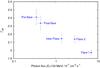 |
Fig. 6 The γ-ray photon index, Γph, as a function of flux for the time periods defined in Table 1. |
| In the text | |
|
Fig. 7 Keck II/DEIMOS spectrum of GB 1310+487. The two narrow-line systems are indicated. The region 6900–7000 Å is lost to a gap between the two CCDs. The slit position is shown in Fig. 2. |
| In the text | |
|
Fig. 8 Radio lightcurve at 15 GHz obtained with the OVRO 40 m telescope (points) supplemented with two 14.6 GHz measurements obtained with the Effelsberg 100 m telescope (square). VLBA measurements of the core (component C0, Table 6) are indicated as diamonds. The two arrows mark the peaks of the γ-ray flares observed by Fermi. |
| In the text | |
|
Fig. 9 VLBA radio image of GB 1310+487 obtained on 2010-12-24 at 15 GHz during the course of the MOJAVE program. The image map peak is 0.206 Jy beam-1 and the first contour is 0.15 mJy beam-1. Adjacent contour levels are separated by a factor of 2. Naturally weighted beam size is indicated at the lower-left corner of the image. Green circles indicate positions and best-fit sizes of the model components presented in Table 6. |
| In the text | |
|
Fig. 10 Quasi-simultaneous radio to γ-ray SED of GB 1310+487 during the two flaring episodes and the post-flare period covered by our multiwavelength observations. The time intervals corresponding to these events are defined in Table 1. |
| In the text | |
Current usage metrics show cumulative count of Article Views (full-text article views including HTML views, PDF and ePub downloads, according to the available data) and Abstracts Views on Vision4Press platform.
Data correspond to usage on the plateform after 2015. The current usage metrics is available 48-96 hours after online publication and is updated daily on week days.
Initial download of the metrics may take a while.