| Issue |
A&A
Volume 564, April 2014
|
|
|---|---|---|
| Article Number | A51 | |
| Number of page(s) | 10 | |
| Section | Planets and planetary systems | |
| DOI | https://doi.org/10.1051/0004-6361/201323322 | |
| Published online | 03 April 2014 | |
Millimetre spectral indices of transition disks and their relation to the cavity radius ⋆
1 Leiden Observatory, Leiden University, PO Box 9513, 2300 RA Leiden, The Netherlands
e-mail: This email address is being protected from spambots. You need JavaScript enabled to view it.
2 Universität Heidelberg, Zentrum für Astronomie, Institut für Theoretische Astrophysik, Albert-Ueberle-Str. 2, 69120 Heidelberg, Germany
3 Laboratoire d’Astrophysique, Observatoire de Grenoble, CNRS/UJF UMR 5571, 414 rue de la Piscine, BP 53, 38041 Grenoble Cedex 9, France
4 Harvard-Smithsonian Center for Astrophysics, 60 Garden Street, Cambridge MA 02138, USA
5 California Institute of Technology, MC 249-17, Pasadena CA 91125, USA
6 INAF – Osservatorio Astrofisico di Arcetri, Largo Fermi 5, 50125 Firenze, Italy
7 School of Cosmic Physics, Dublin Institute for Advanced Studies, 31 Fitzwilliam Place, 2 Dublin, Ireland
8 Max-Planck-Institut für Astronomie, Königstuhl 17, 69117 Heidelberg, Germany
9 European Southern Observatory, Karl-Schwarzschild-Strasse 2, 85748 Garching, Germany
Received: 23 December 2013
Accepted: 24 February 2014
Abstract
Context. Transition disks are protoplanetary disks with inner depleted dust cavities that are excellent candidates for investigating the dust evolution when there is a pressure bump. A pressure bump at the outer edge of the cavity allows dust grains from the outer regions to stop their rapid inward migration towards the star and to efficiently grow to millimetre sizes. Dynamical interactions with planet(s) have been one of the most exciting theories to explain the clearing of the inner disk.
Aims. We look for evidence of millimetre dust particles in transition disks by measuring their spectral index αmm with new and available photometric data. We investigate the influence of the size of the dust depleted cavity on the disk integrated millimetre spectral index.
Methods. We present the 3-mm (100 GHz) photometric observations carried out with the Plateau de Bure Interferometer of four transition disks: LkHα 330, UX Tau A, LRLL 31, and LRLL 67. We used the available values of their fluxes at 345 GHz to calculate their spectral index, as well as the spectral index for a sample of twenty transition disks. We compared the observations with two kinds of models. In the first set of models, we considered coagulation and fragmentation of dust in a disk in which a cavity is formed by a massive planet located at different positions. The second set of models assumes disks with truncated inner parts at different radii and with power-law dust-size distributions, where the maximum size of grains is calculated considering turbulence as the source of destructive collisions.
Results. We show that the integrated spectral index is higher for transition disks (TD) than for regular protoplanetary disks (PD) with mean values of  = 2.70 ± 0.13 and
  = 2.20 ± 0.07 respectively. For transition disks, the probability that the measured spectral index is positively correlated with the cavity radius is 95%. High angular resolution imaging of transition disks is needed to distinguish between the dust trapping scenario and the truncated disk case.
Key words: accretion, accretion disks / protoplanetary disks / circumstellar matter / planets and satellites: formation
The final PdBI data used in the paper are only available at the CDS via anonymous ftp to cdsarc.u-strasbg.fr (130.79.128.5) or via http://cdsarc.u-strasbg.fr/viz-bin/qcat?J/A+A/564/A51
© ESO, 2014
1. Introduction
Observations by infrared telescopes done with e.g. Spitzer and Herschel and by millimetre observations with radio-interferometers such as the Submillimetre Array (SMA), the Very Large Array (VLA) or the Combined Array for Research in Millimeter-wave Astronomy (CARMA) have revealed different types of structures in circumstellar disks surrounding young stars. Transition disks show a lack of mid-infrared radiation in the spectral energy distribution (SED), implying an absence of warm dust in the inner disk (e.g. Calvet et al. 2005; Piétu et al. 2006; Espaillat et al. 2010). Some of these cavities have been resolved by continuum observations (see Williams & Cieza 2011, for a review). The recent discoveries of companion candidates inside transition disks, such as HD 142527 (Biller et al. 2012) and HD169142 (Quanz et al. 2013), promote the idea that holes in transition disks are the result of a brown dwarf, planet, or multiple planets interacting with the disk. However, none of these companion candidates have been confirmed, and alternative explanations have been suggested to explain the observations (Olofsson et al. 2013).
Hydrodynamical simulations of planet-disk interactions have been explored for several years (e.g. Lin & Papaloizou 1979; Paardekooper & Mellema 2004). The presence of a massive planet in a circumstellar disk not only affects the surrounding gas, but also the dust distribution in the disk. A planet of ≳1 MJup opens a gap in a viscous disk and dust can flow through a gap, depending on the particle size and the shape of the gap (Rice et al. 2006; Pinilla et al. 2012a; Zhu et al. 2012, 2013). The overall dust distribution is unknown, and observations at different wavelengths with high sensitivity and resolution are crucial for understanding how dust evolves under disk clearing environments.
Maps of sub-millimetre and microwave emission from the diffuse interstellar dust have shown that the typical values for the dust opacity index βmm are ~1.7–2.0 (see e.g. Finkbeiner et al. 1999). Hence, if the dust in protoplanetary disks is similar to the interstellar medium (ISM) dust, βmm is expected to be similar. However, changes in the opacity between the ISM and denser regions have been found (e.g. Henning et al. 1995). Dust evolution in protoplanetary disks, and especially the process of grain growth to millimetre sizes in the midplane of disks, has been confirmed by observations (see reviews by Natta et al. 2007; Testi et al. 2014). The slope of the SED, known as the spectral index αmm, in the millimetre regime can be interpreted in terms of grains size, via αmm ≈ βmm + 2 (see e.g. Draine 2006), and low values of αmm (≲3.5) correspond to big particles (≳mm). Sub- and millimetre observations of classical protoplanetary disks have shown that the spectral index reaches low values αmm ≲ 3.5 in Taurus, Ophiuchus, Orion, Chamaeleon, Lupus, etc., star forming regions (e.g. Testi et al. 2001, 2003; Rodmann et al. 2006; Lommen et al. 2007, 2009, 2010; Ricci et al. 2010a,b, 2011; Ubach et al. 2012).
Alternative explanations for the low spectral indices in disks have been addressed by different authors. One possible explanation is that the emission or part of the emission may come from unresolved regions where the dust is optically thick at millimetre wavelengths (Testi et al. 2001, 2003), but it has been shown that this is unlikely to be the general explanation for the low values of the opacity index measured in large samples of disks (Ricci et al. 2012b). In addition, the chemical composition (Semenov et al. 2003), porosity (Henning & Stognienko 1996; Stognienko et al. 1996), and geometry of the dust particles can affect the opacity index. However, their impact is not significant, for reasonable values of the properties of the dust grains (see e.g. Draine 2006). Thus, the most likely explanation is that dust grains have grown to mm-sizes (see in addition Calvet et al. 2002; Natta & Testi 2004; Natta et al. 2007).
One of the most critical challenges of planetesimal formation is to understand how the rapid inward migration of dust grains can stop. The theory of radial drift and observations at mm-wavelength are in strong disagreement (e.g. Brauer et al. 2007). The confirmation of long-lived presence of mm grains with observations made theoreticians to look for the missing piece of this rapid inward-drift puzzle. Particle trapping in pressure maxima (i.e. locations where ∇p = 0 and ∇2p < 0) is a result of the dynamic phenomenon that, due to friction with the gas, particles tend to drift in the direction of higher gas pressure, i.e. up the pressure gradient (e.g. Klahr & Henning 1997). Besides the inward drift reduction in pressure bumps, dust grains do not experience the potentially damaging high-velocity collisions due to relative radial and azimuthal drift anymore, thus reducing the fragmentation problem as well.
Pressure bumps may themselves be caused by planets that have formed by a yet unknown mechanism. A possible first planet embryo can be explained by the growth of a seed (cm-sized object) by sticking mutual collisions, including mass transfer and bouncing effects as possible outcomes of the collisions (Windmark et al. 2012). Once a massive planet is formed and opens a gap, a pressure bump is expected in the radial direction at the outer edge of the gap due to the depletion in the gas surface density. This pressure bump becomes a “particle trap”, a region where particles accumulate and grow. This trap is therefore a good planet incubator for the next generation of planets. Particle trapping creates a ring-like emission at mm-wavelengths, whose radial position and structure depend on the disk viscosity, mass, and location of the planet (Pinilla et al. 2012a). In addition, the non-axisymmetric emission of transition disks revealed by sub-mm observations (Brown et al. 2009) and recently confirmed with ALMA and CARMA observations (Casassus et al. 2013; van der Marel et al. 2013; Isella et al. 2013; Fukagawa et al. 2013; Pérez et al. 2014) may also be a result of particle trapping that lead to strong asymmetric maps (Birnstiel et al. 2013; Ataiee et al. 2013; Lyra & Lin 2013).
Spatially resolved, multi-frequency observations will provide crucial information about the dust density distribution of transition disks. Radial variations in the dust opacity have been revealed for individual disks (e.g. Pérez et al. 2012; Trotta et al. 2013); however, a statistical study cannot have been done yet. In this paper, we show that in the case of transition disks, a change in the cavity radius affects the spatially integrated spectral index, a quantity already available for a significant number of transition disks.
We present 3 mm-observations of four transition disks: LkHα 330, UX Tau A, LRLL 31, and LRLL 67 carried out with Plateau de Bure Interferometer (PdBI). The observations and data reduction of our four targets are presented in Sect. 2, together with the information on additional transition disks. Section 3 presents the integrated spectral index of our sample with the data collected from the literature. In this section a comparison between the spectral indices of transition and regular protoplanetary disks is presented, as well as a possible correlation between the cavity radii and the spectral index. In Sect. 4 we compare the observations to two different kinds of models: first of all, dust evolution models based on planet-related cavities, where a pressure bump is formed at the outer edge of the gap, which traps millimetre particles; second, models with a power law size distribution of particles with an artificial cut at different radii to imitate dust cavities. Finally, in Sect. 5 we give the main conclusions of this work.
Observed targets.
2. Observations
2.1. PdBI observations
The observations with PdBI were made on 20 and 21 September of 2012 under excellent weather conditions (seeing of ~1.7′′), using only the WideX correlator. The sample consists of four transition disks: LkHα 330, UX Tau A, LRLL 31, and LRLL 67. These sources were selected based on the 880 μm flux information available (Andrews et al. 2011b; Espaillat et al. 2012), the lack of 3 mm data in the literature, and their position in the sky. The 880 μm imaging of LkHα 330 and UX Tau A has confirmed a dust-depleted cavity for these disks (Brown et al. 2009; Andrews et al. 2011b). There are no resolved images for LRLL 31 and LRLL 67. The available information about the position, stellar parameters, cavity radii, and millimetre fluxes of these targets are summarised in Table 1, with the corresponding references.
The targets were observed in track-sharing mode with constant time intervals, inter-scanned between the science target and quasars observations, including 0333+321 and 0507+179 for phase and amplitude calibration. To calibrate the spectral response of the system, 3C84, 3C345, and 0234+285 were observed as bandpass calibrators. For the absolute flux calibration, MWC349 was used with a fixed flux value of 1.20 Jy at 100.0 GHz. For the data reduction, the Fourier inversion of the visibilities and the cleaning of the dirty image of the dust emission, the Grenoble Image and Line Data Analysis Software (GILDAS) was used. The observations were carried at a frequency of 100.0 GHz with a bandwidth of ~3.6 GHz for continuum (3 mm) and with six antennas in the D-configuration. The D-antenna configuration is the most compact and provides the lowest phase noise and highest sensitivity available using PdBI. In Appendix A, the 3 mm maps for the observed targets, with the corresponding resolution and noise level are presented.
2.2. Additional transition disks
In addition to our own observations, we gathered available photometric data of other transition disks. The summary of this sample is in Table 2 with the corresponding references. The target selection is based on transition disks for which the millimetre flux is known within a good uncertainty at two different and well-separated (sub-) millimetre wavelengths, preferably between ~ 880 μm–1.2 mm and ~ 2.7–3.0 mm. Shorter wavelengths are not taken to avoid possible contribution from optically thick dust. Longer wavelengths are not considered to minimise the contamination from ionised gas.
Most of our selected targets are disks around T Tauri stars, except for the Herbig disks MWC 758 and HD 163296. Table 2 shows the spectral type, accretion rate, cavity radii, and fluxes at millimetre wavelengths. The cavity radius reported in the table has either been resolved by continuum observations (R) or derived from SED (S) fitting. These values of the cavity radii from the SED fitting are degenerate and highly uncertain. Even more important, the cavity size measurements inferred by SED modelling and by mm-observations refer to two different kinds of grains, of micron and millimetre sizes respectively, which do not need to be spatially coexisting. An example where both measurements are available is the transition disk SAO 206462, for which the cavity size in micron size particles is smaller (~28 AU) than what is inferred for large dust grains from mm-observations (39 to 50 AU, Garufi et al. 2013). Scattered light observations of transition disks with high angular resolution are needed to confirm the cavity size and the decoupling of large and small grains predicted indeed by dust evolution models to be observed (de Juan Ovelar et al. 2013).
3. Results
In this section, we present the integrated spectral index for the transition disks sample and the correlation with the cavity size.
Additional data.
3.1. Spectral Index
At mm-wavelengths, the thermal emission of a disk, integrated over its surface, is dominated by the emission of the outer, optically thin region. In the Rayleigh-Jeans limit, the wavelength dependence of the integrated flux can be expressed as Fν ∝ νβmm + 2, where βmm is the opacity index. It can be measured with multi-wavelength observations (βmm ≡ dlnκ/dlnν), and the slope of the SED at long wavelengths can be approximated to αmm ≈ βmm + 2.
Using the 880 μm and 3 mm fluxes of the observed targets and fluxes from literature, we calculated the millimetre spectral indices αmm. Tables 1 and 2 summarise our findings. For calculating of the uncertainties of the spectral indices and the flux at 1 mm, besides the noise level or rms (σ) of the observations, a systematic error from the flux calibration is included. It is taken to be 15% of the total flux, since it is estimated from measurements with different instruments, such as CARMA, PdBI, and SMA (see e.g. Ricci et al. 2011).
Analysis of recent mm-observations at different wavelengths of several protoplanetary disks have shown that the opacity index may change with radius (Isella et al. 2010; Guilloteau et al. 2011; Pérez et al. 2012; Trotta et al. 2013). For instance, Guilloteau et al. (2011) investigated a total of 23 disks in Taurus-Auriga region and found that for nine sources, βmm increases with radius, implying that dust grains are larger in the inner disk (≲100 AU), where the gas density is higher, than beyond. If one assumes that transition disks had the same grain population before a clearing mechanism acted on them and also that the opacity index increases with radius (e.g. Guilloteau et al. 2011), it is expected that disks with cavities lack large grains in the inner disk (r < Rcav) and therefore have higher values of the integrated spectral index than typical disks.
To compare the integrated spectral index of regular protoplanetary disks and transition disks, we use the data from Ricci et al. (2012a), who presented millimetre fluxes and spectral indices of a total of ~50 disks in Taurus, Ophiuchus, and Orion star forming regions. The transition disk population includes disks in different star forming regions such as Taurus, Perseus, Lupus, Ophiuchus, and, among others. Figure 1 shows the differences between the two distributions (plotted with the same number of bins), with a mean value of the spectral index for typical protoplanetary disks and for transition disks. This comparison indicates that the millimetre index for transition disks is in average higher than for protoplanetary disks.
In addition, to compare the two samples, we calculate the Kolmogorov-Smirnov (KS) two-sided test, finding that the maximum deviation between the cumulative distributions is 0.66 with a significance level of 5.11 × 10⁻⁶, i.e. with a very low probability (≪1%) that the two samples are similar1 Moreover, we calculate the significance level 1000 times, considering random values for the uncertainties of the spectral index within the corresponding error bars for both samples, finding a very low mean probability that the two distributions are similar (less than 1%).
3.2. Correlation of the spectral index and the cavity size
The integrated spectral index αmm of the four observed transition disks is lower than 3.5, although in some cases, αmm is close to the mean value for the ISM. The large value of αmm for LkHα 330 is confirmed by Isella et al. (2013), who report CARMA observations at 1.3 mm of this transition disk and obtain α0.88 − 1.3 mm = 3.6 ± 0.5. This can be interpreted as no-grain growth, if one assumes constant values of βmm over the whole disk. From our observed targets, LkHα 330 is the disk with the largest estimated inner hole, ~ 68 AU (Andrews et al. 2011a). LRLL 31 and UXTau A have lower spectral indices and smaller inner holes, 14 and 25 AU respectively (Andrews et al. 2011a; Espaillat et al. 2012). The spectral index of LRLL67 has a large error, preventing any conclusion on the relation between its integrated spectral index and the cavity radii.
Considering the sample of all transition disks (Tables 1 and 2), Fig. 2 shows the correlation between the spectral index and the cavity radius. For the uncertainties of the cavity radius, we consider an uncertainty of 40% for the cavity radii when they are derived from SED fitting. This error may be underestimated due to the high degeneracy from the SED modelling. When the cavities are resolved, an error of ±5 AU is considered (~20% of the resolution obtained from continuum observations at typical distances of ~140 pc, see for example Andrews et al. 2011a). Figure 2 also shows the linear regression from the data using a Bayesian method introduced by Kelly (2007), which includes measurement errors of the data in both Rcav and αmm, as well as intrinsic scatter. Fitting a linear relationship between the spectral index and the cavity radius, such that αmm = a × Rcav + b, we find a = 0.011 ± 0.007 and b = 2.36 ± 0.28. We show the 95% (2σ) confidence interval and the 68% (1σ) confidence region on the regression line. All data from observations, when error bars are included, are contained within 95% confidence interval. According to Kelly (2007), 5000 iterations should be enough for the convergence of the linear coefficients. We assume 100 000 iterations and took the last 95 000 values to ensure a good convergence of our estimations. This analysis shows that the probability of a positive correlation, considering uncertainties and scattering of the data, is ~95%. We repeat this linear regression assuming a higher uncertainty (50%) for the cavity radii obtained by SED modelling, finding that the probability of a positive correlation decreases by less than 1%.
To determine whether the best fitting of the points in Fig. 2 is linear, we use the χ2 test for several polynomial functions, finding that the best fit to the data is obtained using linear fitting. The changes for χ2 for higher polynomial orders are less than 1% compared to the linear fitting. This suggests that any additional order above the linear polynomial, which we can take to model our observations, is over fitting the data.
The statistics remain low, but these observations suggest a positive dependence between αmm and the cavity radius. Observations with better resolution and sensitivity are needed to refine this analysis and to determine an accurate relation between Rcav and αmm.
 |
Fig. 1 Comparison of the normalised distribution of the integrated spectral index for classical disks (data from Ricci et al. 2012a) and transition disks (data in Tables 1 and 2), using the same number of bins for each case. |
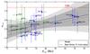 |
Fig. 2 Spectral indices αmm vs. the cavity radius for the observed transition disks. Data from our PdBI observations and available data from the literature are plotted (data in Tables 1 and 2). Triangle points correspond to sources for which the cavity radius is inferred from SED modelling, while circle points correspond to resolved cavities by continuum observations. The uncertainties on the cavity radii are taken to be 40% of the mean value in the case of SED modelling and 5 AU for the resolved cavities. The dashed line corresponds to the linear regression from the data using the method introduced by Kelly (2007). The shaded regions show the 95% (2σ) confidence interval (lighter) and the 68% (1σ) confidence region (darker) on the regression line. The dot-dashed line represents the best linear regression from the models described in Sect. 4. |
4. Discussion
Transition disks show a wide range of properties such as the extent of the observed inner holes from 4 AU to even more than 100 AU, relatively high accretion rates (~ 10-8 M⊙ yr-1), and averaged lifetimes (~1–3 Myr), among others (see Williams & Cieza 2011, for a review). Recently, different studies have combined various physical models to explain these properties. For instance, Rosotti et al. (2013) combined X-ray photoevaporation models with planet-disk interactions to investigate the transition disks with accretion rates comparable to classical T-Tauri stars and large inner holes. On the other hand, Pinilla et al. (2012a) studied how the dust evolves in a disk that is perturbed by the presence of a massive planet. In that work, they demonstrate that the ring-shaped emission of some transition disks can be modelled using a single planet. The radial location of the mm-sized particles depends on the shape of the resulting gap, which is determined by the disk viscosity, mass, and location of the planet. Other models such as a vortex generated by a dead zone (Regály et al. 2012), a region in the disk where the viscosity drops down, may also explain some of the observed features of transition disks (Brown et al. 2009; Isella et al. 2013). In this section, in order to distinguish between the dust trapping scenario and a truncated disk case, we compared the observations presented in Sect. 3 with two different kind sof models. In the first set of models, we consider coagulation and fragmentation of dust particles in a disk with a cavity carved by a massive planet and with particle trap being at the outer edge of the cavity. In the second set of models, we assume a truncated disk at different radii without the computation of the dust evolution, but a power law for the size distribution of particles.
4.1. Models of grain growth in transition disks
 |
Fig. 3 Top panel: dust surface density calculated from simulations in Pinilla et al. (2012a) and considering grain sizes (a) from 1 to 100 mm after 1 Myr of evolution. The disk hosts a massive planet at 20 AU. In the case of 1 MJup (dashed line), the peak of dust surface density is at ~ Rcav ~ 30 AU, the spectral index is α1 − 3 mm = 2.4, while for 15 MJup and the peak of the dust surface density at ~ Rcav ~ 55 AU (solid line), the spectral index is α1 − 3 mm = 2.8. The dash-dotted line represents the dust surface density with the same grain sizes in a protoplanetary disk without a planet, but after suppression of the radial drift. Bottom panel: as top panel, but for micron-sized particles. |
In our dust evolution models (Birnstiel et al. 2010a), dust densities evolve due to radial drift, turbulent mixing, and gas drag. At the same time, particles coagulate, fragment, and erode depending on their relative velocities. The sources for relative velocities are Brownian motion, turbulence, radial drift, and vertical settling. The final dust density distribution depends on disk parameters, such as the gas surface density, and viscosity; particle parameters like fragmentation velocity and the intrinsic volume density of the spherical grains (see Birnstiel et al. 2010a, for more details). In the case of a massive planet interacting with the disk, the gas surface density is calculated from simulations using the polar hydrodynamic code FARGO (Masset 2000), after the disk evolves during ~ 1000 planet orbits. For the results present in this section, the disk parameters are assumed as in Pinilla et al. (2012a), i.e., a disk around a Solar-type star, with a flared geometry and viscosity parameter αturb = 10-3. The disk mass is taken to be 0.05 M⊙ and the inner and outer radius of the disk change depending on the position of the planet, to have a disk extended from 1 to 150 AU.
When a single massive planet is interacting with the disk, it is expected that dust particles accumulate and grow to mm-sizes at distances that can be even twice or more than the star-planet separation. As a consequence, for a transition disk in which cavity is the result of a planet within the disk, the inner part (r < Rcav) can be completely depleted of mm-grains depending on the planet mass. The top panel of Fig. 3 shows the radial variation in the dust surface density Σdust from the simulations presented in Pinilla et al. (2012a), calculated only for millimetre particles i.e. 1–100 mm (top panel), for the cases of a 1 and 15 MJup planet located at 20 AU. The case of a typical protoplanetary disk around a T Tauri star where the radial drift is reduced without any gas density perturbation (i.e. no pressure bump(s)) is also shown in Fig. 3. The bottom panel of Fig. 3 shows for comparison the dust density for micron-sized particles (1–10 μm) under the same conditions. All results are shown after 1 Myr of evolution. The comparison between the two panels of Fig. 3 shows that micron-sized particles are trapped less efficiently than mm-sized particles, leading to spatial differences in the dust size distribution.
The grain growth process under the presence of a pressure bump can lead to significant radial variations of the opacity. When the inner disk is almost depleted of mm-grains, as we notice in Fig. 3 for the 1 and 15 MJup planet cases, the opacity index is high in the inner region and low in the outer part of the disk where the dust grains are trapped. This result contrasts with the findings on typical protoplanetary disks, where βmm increases with radius (Guilloteau et al. 2011; Pérez et al. 2012; Trotta et al. 2013). In fact, the radial variation of βmm for regular disks is expected to be inverse to the variation in the dust surface density of mm-grains, i.e. low values for βmm in the inner region (r ≲ 70 AU) and higher in the outer part.
4.2. Comparison with observations
To calculate the disk-integrated spectral index αmm for a transition disk in this model, we considered dust density distributions after 1 Myr of dust evolution as in Fig. 3. We calculated the opacities κν for each grain size at a given frequency ν, assuming the optical constants for magnesium-iron silicates (Jaeger et al. 1994; Dorschner et al. 1995) from the Jena database2 and using Mie theory. The grid for the particle sizes runs from 1 μm to 200 cm. Once the opacities were calculated, the optical depth τν was computed as  (1)where σ(r,a) is the total dust surface density and i the disk inclination. The flux of the disk at a given frequency Fν is therefore
 ![Mathematical equation: \begin{equation} F_\nu=\frac{2\pi\cos{i}}{d^2}\int_{R_{\mathrm{in}}}^{R_{\mathrm{out}}} B_\nu(T(r)) [1-{\rm e}^{-\tau_\nu}] r {\rm d}r, \label{eq:flux} \end{equation}](/articles/aa/full_html/2014/04/aa23322-13/aa23322-13-eq147.png) (2)with d the distance to the source and Bν(T(r)) the Planck function for a given temperature profile T(r). The temperature is calculated self-consistently between the hydrodynamical simulations, the dust evolution, and the calculation of the millimetre fluxes. The millimetre emission computed from the dust density distribution that results from the dust evolution models is optically thin. Thus, the variations of the integrated millimetre spectral index exclusively come from different dust size distributions in each case, since in our models the disk is in the Rayleigh-Jeans regime for all radii.
(2)with d the distance to the source and Bν(T(r)) the Planck function for a given temperature profile T(r). The temperature is calculated self-consistently between the hydrodynamical simulations, the dust evolution, and the calculation of the millimetre fluxes. The millimetre emission computed from the dust density distribution that results from the dust evolution models is optically thin. Thus, the variations of the integrated millimetre spectral index exclusively come from different dust size distributions in each case, since in our models the disk is in the Rayleigh-Jeans regime for all radii.
All spectral indices are calculated assuming the same disk and dust parameters. These parameters are a disk around a typical T Tauri star of 1M⊙ mass, whose mass is Mdisk = 0.05 M⊙, a viscosity parameter of αturb = 10-3, fragmentation velocities of particles of 10 m s-1, and the same initial dust surface density. The intrinsic volume density ρs of a spherical grain is taken to be 1.2 g cm-3. The effect of each of these parameters on the opacity index was investigated in detail by Birnstiel et al. (2010b) and Pinilla et al. (2013), and it will be discussed later. We consider d = 140 pc and i = 0 (face-on disks). The cavity radius depends on the mass and planet location, and we focus on these two variables to study the effect that the cavity shape has on the value of αmm.
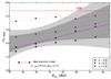 |
Fig. 4 Disk-integrated spectral index α1 − 3 mm vs. the cavity radius for two different kind of models: (1) dust evolution in a disk holding a 1 MJup located at different distances and created different cavity size (stars in the plot). For this case, the best linear fit to this model is also plotted (dashed line). (2) Models without considering dust evolution, but a dust-rich disk, assuming a power-law grain size distribution (n(a) ∝ a− s), with amin = 1 μm, amax given by Eq. (3), three different values for s (s = 3.0, square points; s = 3.5 triangle points, and s = 4.0 circle points), and different truncated radii. The 1 and 2 σ regions from observations (Fig. 2) are also plotted. |
Effect of the planet mass.
For our research, we calculated the millimetre fluxes at 1 and 3 mm using Eq. (2). In this case, we considered two cases of 1 MJup and 15 MJup located at the same orbital distance (20 AU as in Fig. 3). The disk integrated spectral index for the 1 MJup and Rcav ~ 30 AU is α1 − 3 mm = 2.4, while for 15 MJup and Rcav ~ 55 AU, it is α1 − 3 mm = 2.8. The cavity radius Rcav is taken to be where the peak of the dust surface density is located and observed at mm-wavelenghts. Increasing the cavity radii by more than 20 AU using a more massive planet increases the value of the integrated spectral index as well.
When a single massive planet interacts with the disk, the size of the resulting cavity at mm-wavelengths can be written in terms of the Hill planet radius rH, defined as rH = rp (Mp/3M⋆)1/3, where rp and Mp are the radial position and mass of the planet. For 1 MJup < Mp < 5 MJup, the mm-emission is expected to be at ~ 7 rH, while for a disk hosting a more massive planet, the emission is expected at ~ 10 rH (Pinilla et al. 2012a). Increasing the planet mass is therefore not as effective as increasing the planet location to create wide cavities. For this reason a factor of 15, for example, in the planet mass has a moderate effect on the integrated spectral index.
Effect of the planet location.
To investigate the influence of the planet location, we restrict our analysis to the the case of 1 MJup located at six different positions from rp = 10 AU to rp = 60 AU. In this case, the mm-cavity is in a range of Rcav = 20–90 AU. Figure 4 shows the integrated spectral index vs. the cavity radius from simulations. The results confirm that indeed αmm linearly increases with the cavity radius. Figure 4 also shows the best linear fit of the model prediction, which minimises the squared error χ2: α1−3 mm = 0.012 × Rcav + 2.15. This fit is over-plotted in Fig. 2 and shows that this model fit explains the observations well.
The increase in αmm with Rcav is because the disk integrated emission is dominated by the dust at Rcav in the pressure trap, in which the maximum size of particles decreases when Rcav is further from the star. When the radial drift is reduced in a particle trap, turbulent motion is the main source of destructive collisions. As a result, the maximum size of the particles amax is reached when the fragmentation velocity of the particles vf is equal to the turbulent relative velocity. In this case, amax scales with the gas surface density Σg as (Birnstiel et al. 2010a)  (3)where αturb is a turbulence parameter, ρs the mass density of a single grain, and cs the sound speed. Equation (3) implies that the maximum size that particles reach in the coagulation/fragmentation cycle decreases with radius as the gas surface density does. Moreover, the size of the particles that are perfectly trapped (acritical) in a pressure bump (P) also scales with the gas surface density as (Pinilla et al. 2012b)
  (4)Therefore, for disks with similar parameters, but with the pressure bump located further out from the star (wider cavity), amax and acritical are expected to be smaller. For instance, for the parameters considered in this model, we have amax ~ 10 cm at 50 AU, while at 100 AU amax ~ 1 cm, leading to higher values of the integrated spectral index as shown in Fig. 4.
Effect of other parameters.
Disk and stellar parameters also influence the integrated spectral index, such as disk and stellar mass, turbulence, and disk size. For instance, if the disk mass decreases, this also decreases the millimetre fluxes and the maximum size of particles (because Σg also decreases, if the gas surface density profile remains the same, Eq. (3)). As a consequence, the integrated spectral index is expected to be higher for low mass disks (Birnstiel et al. 2010b). Variations in the gas surface density profile, keeping the same disk mass, do not have a significant influence on αmm (Pinilla et al. 2013). On the other hand, radial drift is more efficient for particles around low-mass stars, and millimetre grains around low-mass stars stay in the outer regions during shorter times than around solar-type stars (Pinilla et al. 2013). Disk turbulence also affects the maximum grain size, and low values of αturb allow larger grains and decrease the spectral index. Similarly, if the threshold velocity for destructive collision increases i.e. if vf is higher, then particles would reach larger sizes (Eq. (3)). As a consequence, varying those parameters would change the slope and the intercept of the linear relation and broaden the correlation found by dust evolution modelling.
 |
Fig. A.1 Continuum maps at 100.50 GHz (3 mm) obtained with the PdBI observations with contour lines every 2σ. Upper left panel: LkHα 330 with σ = 0.12 mJy/beam, beam size of 5.01″ × 3.69″ and position angle of the major axis of 117°. Upper right panel: UX Tau A with σ = 0.33 mJy/beam, beam size of 6.36″ × 3.54″ and position angle of the major axis of 125°. Bottom left panel: LRLL 31 with σ = 0.08 mJy/beam, beam size of 5.05″ × 3.66″ and position angle of the major axis of 117°. Bottom right panel: LRLL 67 with σ = 0.09 mJy/beam, beam size of 4.98″ × 3.67″ and position angle of the major axis of 116°. The beam is shown in the bottom right of each image. |
4.3. Truncated disk
To compare our previous results that include the computation of the dust coagulation/fragmentation with a truncated dust-rich disk, we consider a power-law grain size distribution given by n(a) ∝ a− s with amin = 1 μm, amax scaling as in Eq. (3), and s taken to be s = [3,3.5,4]. For T, αturb, vf, and ρs, the same values are taken as in the dust evolution models. The gas surface density is taken as in Lynden-Bell & Pringle (1974), ![Mathematical equation: \begin{equation} \Sigma_{\rm g}(r)=\Sigma_0 \left(\frac{r}{r_{\rm c}}\right)^{-\gamma} \exp \left[-\left(\frac{r}{r_{\rm c}}\right)^{2-\gamma}\right], \label{density} \end{equation}](/articles/aa/full_html/2014/04/aa23322-13/aa23322-13-eq201.png) (5)where rc is the characteristic radius assumed to be 60 AU, Σ0 is calculated such that the disk mass is 0.05 M⊙, and γ is equal to 1. Since the shape of the gas surface density does not significantly influence the integrated spectral index, variations in the characteristic radius and γ are not considered. To mimic different cavity sizes and study the effect of just removing the optically thick inner disk on the integrated spectral index, an artificial cut at different radii is done, inside which the disk is empty of dust. Using the same procedure of Sect. 4.2 to calculate the millimetre fluxes, Fig. 4 shows the correlation between the integrated spectral index and disks with different cavity sizes.
(5)where rc is the characteristic radius assumed to be 60 AU, Σ0 is calculated such that the disk mass is 0.05 M⊙, and γ is equal to 1. Since the shape of the gas surface density does not significantly influence the integrated spectral index, variations in the characteristic radius and γ are not considered. To mimic different cavity sizes and study the effect of just removing the optically thick inner disk on the integrated spectral index, an artificial cut at different radii is done, inside which the disk is empty of dust. Using the same procedure of Sect. 4.2 to calculate the millimetre fluxes, Fig. 4 shows the correlation between the integrated spectral index and disks with different cavity sizes.
Increasing the slope of the size grain distribution s, implies less large grains and higher values of αmm. For this reason, in the cases of s = 3.5 and s = 4, the spectral index is high compare with the dust evolution models. Only in the case of s = 3.0, does α1 − 3 mm reach low values and converge almost to the same value as in the dust evolution models for a disk without a cavity (Rcav → 0, see Fig. 4). Considering different values for Mdisk, αturb, and vf, the corresponding variations in the spectral index are as expected from the models that include the computation of dust evolution. This is because the maximum grain size is computed following Eq. (3), which assumes that turbulence causes destructive collisions, as in the case of the coagulation/fragmentation calculation with reduced radial drift.
The two frameworks presented in this work, the planet-disk interaction with dust evolution and a truncated disk with a power law size distribution, remain possible explanations for the positive trend obtained by observations (Fig. 4). However, combinations of scatter light and millimetre wavelength observations, with high angular resolution, of transition disks will distinguish between the two scenarios (de Juan Ovelar et al. 2013).
5. Summary and conclusions
We have reported 3 mm observations carried out with PdBI of four transition disks LkHα 330, UX-Tau A, LRLL 31, and LRLL 67. Using previous observations of these targets at 880 μm, we calculated the spectral index, and found that for these sources the values for αmm are lower than typical values of the ISM dust. However, the disk-integrated spectral index αmm is close to the value for ISM-dust (~3.7) for LkHα 330 (αmm = 3.25 ± 0.40), which is also the target with the largest inner hole (~68 AU, Andrews et al. 2011b). The sources UX-Tau A and LRLL 31 have smaller cavity radii of 25 AU and 14 AU, respectively, and lower integrated spectral indices, αmm = 2.20 ± 0.40 for UX-Tau A and αmm = 2.50 ± 0.44 for LRLL 31. Owing to the large uncertainties on the millimetre flux of LRLL 67, there is no conclusive correlation between the integrated spectral index and its cavity radius.
Recent observations at different wavelengths have shown that the opacity may change radially throughout the disk (Isella et al. 2010; Guilloteau et al. 2011; Pérez et al. 2012; Trotta et al. 2013). Studies that combine dust evolution and planet-disk interaction for transition disks (Pinilla et al. 2012a) indicate that the dust size distribution may present strong spatial variations. In this picture, the inner part is depleted of mm grains leading to radial variations of the dust opacity. Thus, the opacity index has higher values in the inner regions than the outer regions, in contrast to observations of classical protoplanetary disks. From models that combine hydrodynamical simulations and dust evolution models for the planet-related cavities, a linear relation between the disk integrated spectral index and the cavity radius is inferred, because the millimetre emission is dominated by the dust at the outer edge of the cavity, i.e. in the pressure bump. This suggests that the spectral index is higher for larger cavities.
Since our own sample is too small to draw statistically significant conclusions, we compiled all the known millimetre fluxes from transition disk sources for which these data exist at least for two separated millimetre wavelengths. Together with our observations, we collecteded a total of twenty transition disks for which the cavity radii are known either by SED modelling or spatially resolved observations, and we calculate the disk integrated spectral indices. We found that the integrated spectral index is higher for transition disks than for regular protoplanetary disks.
Moreover, the probability of a positive trend between the spectral index and cavity size is ~95% (Fig. 2). Two models are considered in this work to explain this positive correlation: first of all, coagulation and fragmentation of dust in a disk whose cavity is formed by a massive planet located at different positions; second, a disk with different truncation radii and with a power-law dust-size distribution where turbulence sets the maximum grain size. Both models can explain the trend, and multi-wavelength observations with high angular resolution are needed to distinguish between the two cases.
Observations with new telescope arrays such as ALMA, EVLA, and NOEMA will provide enough sensitivity and angular resolution to detect the small cavities of many transition disks and constrain the dust opacity distribution of those disks in more detail. Together with scattered imaging, these observations will help us understand the correlation between the spectral index and disk properties, such as the cavity size, hence, the environment where the planets are born.
For the histogram (Fig. 1) and the K-S test, when the sources are repeated in both samples, we only consider them for the transition disk distribution. These targets are DM Tau, GM Aur, SR 21, and DoAr 44.
Acknowledgments
The authors are very thankful to J. M. Winters for his help understanding GILDAS for the PdBI data reduction. We acknowledge S. Andrews, N. van der Marel, and E. van Dishoeck for the helpful comments and feedback on the manuscript. TB acknowledges support from NASA Origins of Solar Systems grant NNX12AJ04G. This publication is based on observations carried out with the IRAM Plateau de Bure Interferometer. IRAM is supported by INSU/CNRS (France), MPG (Germany), and IGN (Spain).
References
- Andrews, S. M., Rosenfeld, K. A., Wilner, D. J., & Bremer, M. 2011a, ApJ, 742, L5 [NASA ADS] [CrossRef] [Google Scholar]
- Andrews, S. M., Wilner, D. J., Espaillat, C., et al. 2011b, ApJ, 732, 42 [NASA ADS] [CrossRef] [Google Scholar]
- Andrews, S. M., Wilner, D. J., Hughes, A. M., et al. 2012, ApJ, 744, 162 [NASA ADS] [CrossRef] [Google Scholar]
- Ataiee, S., Pinilla, P., Zsom, A., et al. 2013, A&A, 553, L3 [NASA ADS] [CrossRef] [EDP Sciences] [Google Scholar]
- Biller, B., Lacour, S., Juhász, A., et al. 2012, ApJ, 753, L38 [NASA ADS] [CrossRef] [Google Scholar]
- Birnstiel, T., Dullemond, C. P., & Brauer, F. 2010a, A&A, 513, A79 [NASA ADS] [CrossRef] [EDP Sciences] [Google Scholar]
- Birnstiel, T., Ricci, L., Trotta, F., et al. 2010b, A&A, 516, L14 [NASA ADS] [CrossRef] [EDP Sciences] [Google Scholar]
- Birnstiel, T., Dullemond, C. P., & Pinilla, P. 2013, A&A, 550, L8 [NASA ADS] [CrossRef] [EDP Sciences] [Google Scholar]
- Brauer, F., Dullemond, C. P., Johansen, A., et al. 2007, A&A, 469, 1169 [NASA ADS] [CrossRef] [EDP Sciences] [Google Scholar]
- Brown, J. M., Blake, G. A., Dullemond, C. P., et al. 2007, ApJ, 664, L107 [NASA ADS] [CrossRef] [Google Scholar]
- Brown, J. M., Blake, G. A., Qi, C., Dullemond, C. P., & Wilner, D. J. 2008, ApJ, 675, L109 [NASA ADS] [CrossRef] [Google Scholar]
- Brown, J. M., Blake, G. A., Qi, C., et al. 2009, ApJ, 704, 496 [NASA ADS] [CrossRef] [Google Scholar]
- Brown, J. M., Rosenfeld, K. A., Andrews, S. M., Wilner, D. J., & van Dishoeck, E. F. 2012, ApJ, 758, L30 [NASA ADS] [CrossRef] [Google Scholar]
- Calvet, N., D’Alessio, P., Hartmann, L., et al. 2002, Apj, 568, 1008 [Google Scholar]
- Calvet, N., D’Alessio, P., Watson, D. M., et al. 2005, ApJ, 630, L185 [NASA ADS] [CrossRef] [Google Scholar]
- Casassus, S., van der Plas, G., M, S. P., et al. 2013, Nature, 493, 191 [NASA ADS] [CrossRef] [Google Scholar]
- de Juan Ovelar, M., Min, M., Dominik, C., et al. 2013, A&A, 560, A111 [NASA ADS] [CrossRef] [EDP Sciences] [Google Scholar]
- Draine, B. T. 2006, ApJ, 636, 1114 [NASA ADS] [CrossRef] [Google Scholar]
- Dorschner, J., Begemann, B., Henning, T., Jaeger, C., & Mutschke, H. 1995, A&A, 300, 503 [NASA ADS] [Google Scholar]
- Espaillat, C., D’Alessio, P., Hernández, J., et al. 2010, ApJ, 717, 441 [NASA ADS] [CrossRef] [Google Scholar]
- Espaillat, C., Furlan, E., D’Alessio, P., et al. 2011, ApJ, 728, 4 [Google Scholar]
- Espaillat, C., Ingleby, L., Hernández, J., et al. 2012, ApJ, 747, 103 [NASA ADS] [CrossRef] [Google Scholar]
- Finkbeiner, D. P., Davis, M., & Schlegel, D. J. 1999, ApJ, 524, 867 [NASA ADS] [CrossRef] [Google Scholar]
- Fukagawa, M., Tsukagoshi, T., Momose, M., et al. 2013, PASJ, 65, L14 [NASA ADS] [CrossRef] [Google Scholar]
- Furlan, E., Hartmann, L., Calvet, N., et al. 2006, ApJS, 165, 568 [NASA ADS] [CrossRef] [MathSciNet] [Google Scholar]
- Garufi, A., Quanz, S. P., Avenhaus, H., et al. 2013, A&A, 560, A105 [NASA ADS] [CrossRef] [EDP Sciences] [Google Scholar]
- Guilloteau, S., Dutrey, A., Piétu, V., & Boehler, Y. 2011, A&A, 529, A105 [NASA ADS] [CrossRef] [EDP Sciences] [Google Scholar]
- Henning, T., & Stognienko, R. 1996, A&A, 311, 291 [NASA ADS] [Google Scholar]
- Henning, T., Michel, B., & Stognienko, R. 1995, Planet. Space Sci., 43, 1333 [NASA ADS] [CrossRef] [Google Scholar]
- Isella, A., Testi, L., Natta, A., et al. 2007, A&A, 469, 213 [CrossRef] [EDP Sciences] [Google Scholar]
- Isella, A., Carpenter, J. M., & Sargent, A. I. 2010, ApJ, 714, 1746 [NASA ADS] [CrossRef] [Google Scholar]
- Isella, A., Pérez, L. M., & Carpenter, J. M. 2012, ApJ, 747, 136 [NASA ADS] [CrossRef] [Google Scholar]
- Isella, A., Pérez, L. M., Carpenter, J. M., et al. 2013, ApJ, 775, 30 [NASA ADS] [CrossRef] [MathSciNet] [Google Scholar]
- Jaeger, C., Mutschke, H., Begemann, B., Dorschner, J., & Henning, T. 1994, A&A, 292, 641 [Google Scholar]
- Klahr, H. H., & Henning, T. 1997, Icarus, 128, 213 [NASA ADS] [CrossRef] [Google Scholar]
- Kelly, B. C. 2007, ApJ, 665, 1489 [NASA ADS] [CrossRef] [Google Scholar]
- Lin, D. N. C., & Papaloizou, J. 1979, MNRAS, 186, 799 [NASA ADS] [CrossRef] [Google Scholar]
- Lommen, D., Wright, C. M., Maddison, S. T., et al. 2007, A&A, 462, 211 [NASA ADS] [CrossRef] [EDP Sciences] [Google Scholar]
- Lommen, D., Maddison, S. T., Wright, C. M., et al. 2009, A&A, 495, 869 [NASA ADS] [CrossRef] [EDP Sciences] [Google Scholar]
- Lommen, D. J. P., van Dishoeck, E. F., Wright, C. M., et al. 2010, A&A, 515, A77 [NASA ADS] [CrossRef] [EDP Sciences] [Google Scholar]
- Lynden-Bell, D., & Pringle, J. E. 1974, MNRAS, 168, 60 [Google Scholar]
- Lyra, W., & Lin, M.-K. 2013, ApJ, 775, 17 [NASA ADS] [CrossRef] [Google Scholar]
- Mathews, G. S., Williams, J. P., & Ménard, F. 2012, ApJ, 753, 59 [NASA ADS] [CrossRef] [Google Scholar]
- McCabe, C., Ghez, A. M., Prato, L., et al. 2006, ApJ, 636, 932 [NASA ADS] [CrossRef] [Google Scholar]
- Masset, F. 2000, A&AS, 141, 165 [NASA ADS] [CrossRef] [EDP Sciences] [Google Scholar]
- Natta, A., & Testi, L. 2004, Star Formation in the Interstellar Medium: In Honor of David Hollenbach, ASP Conf. Proc., 323, 279 [Google Scholar]
- Natta, A., Testi, L., Calvet, N., et al. 2007, in Protostars and Planets V (Tucson: University of Arizona Press), 767 [Google Scholar]
- Olofsson, J., Benisty, M., Le Bouquin, J.-B., et al. 2013, A&A, 552, A4 [NASA ADS] [CrossRef] [EDP Sciences] [Google Scholar]
- Owen, J. E., & Clarke, C. J. 2012, MNRAS, 426, L96 [NASA ADS] [CrossRef] [Google Scholar]
- Paardekooper, S.-J., & Mellema, G. 2004, A&A, 425, L9 [NASA ADS] [CrossRef] [EDP Sciences] [Google Scholar]
- Pérez, L. M., Carpenter, J. M., Chandler, C. J., et al. 2012, ApJ, 760, L17 [NASA ADS] [CrossRef] [Google Scholar]
- Pérez, L. M., Isella, A., Carpenter, J. M., & Chandler, C. J. 2014, ApJ, 783, L13 [NASA ADS] [CrossRef] [Google Scholar]
- Piétu, V., Dutrey, A., Guilloteau, S., Chapillon, E., & Pety, J. 2006, A&A, 460, L43 [NASA ADS] [CrossRef] [EDP Sciences] [Google Scholar]
- Pinilla, P., Benisty, M., & Birnstiel, T. 2012a, A&A, 545, A81 [NASA ADS] [CrossRef] [EDP Sciences] [Google Scholar]
- Pinilla, P., Birnstiel, T., Ricci, L., et al. 2012b, A&A, 538, A114 [NASA ADS] [CrossRef] [EDP Sciences] [Google Scholar]
- Pinilla, P., Birnstiel, T., Benisty, M., et al. 2013, A&A, 554, A95 [NASA ADS] [CrossRef] [EDP Sciences] [Google Scholar]
- Qi, C., D’Alessio, P., Öberg, K. I., et al. 2011, ApJ, 740, 84 [NASA ADS] [CrossRef] [Google Scholar]
- Quanz, S. P., Avenhaus, H., Buenzli, E., et al. 2013, ApJ, 766, L2 [NASA ADS] [CrossRef] [Google Scholar]
- Regály, Z., Juhász, A., Sándor, Z., & Dullemond, C. P. 2012, MNRAS, 419, 1701 [NASA ADS] [CrossRef] [Google Scholar]
- Rice, W. K. M., Armitage, P. J., Wood, K., & Lodato, G. 2006, MNRAS, 373, 1619 [NASA ADS] [CrossRef] [Google Scholar]
- Ricci, L., Testi, L., Natta, A., et al. 2010a, A&A, 512, A15 [NASA ADS] [CrossRef] [EDP Sciences] [Google Scholar]
- Ricci, L., Testi, L., Natta, A., & Brooks, K. J. 2010b, A&A, 521, A66 [NASA ADS] [CrossRef] [EDP Sciences] [Google Scholar]
- Ricci, L., Mann, R. K., Testi, L., et al. 2011, A&A, 525, A81 [NASA ADS] [CrossRef] [EDP Sciences] [Google Scholar]
- Ricci, L., Testi, L., Natta, A., Scholz, A., & de Gregorio-Monsalvo, I. 2012a, ApJ, 761, L20 [NASA ADS] [CrossRef] [Google Scholar]
- Ricci, L., Trotta, F., Testi, L., et al. 2012b, A&A, 540, A6 [NASA ADS] [CrossRef] [EDP Sciences] [Google Scholar]
- Rodmann, J., Henning, T., Chandler, C. J., Mundy, L. G., & Wilner, D. J. 2006, A&A, 446, 211 [NASA ADS] [CrossRef] [EDP Sciences] [Google Scholar]
- Rosotti, G. P., Ercolano, B., Owen, J. E., & Armitage, P. J. 2013, MNRAS, 430, 1392 [NASA ADS] [CrossRef] [Google Scholar]
- Semenov, D., Henning, T., Helling, C., Ilgner, M., & Sedlmayr, E. 2003, A&A, 410, 611 [NASA ADS] [CrossRef] [EDP Sciences] [Google Scholar]
- Stognienko, R., Henning, T., & Ossenkopf, V. 1996, IAU Colloq. 150: Physics, Chemistry, and Dynamics of Interplanetary Dust, ASP Conf. Ser., 104, 427 [NASA ADS] [Google Scholar]
- Testi, L., Natta, A., Shepherd, D. S., & Wilner, D. J. 2001, ApJ, 554, 1087 [Google Scholar]
- Testi, L., Natta, A., Shepherd, D. S., & Wilner, D. J. 2003, A&A, 403, 323 [NASA ADS] [CrossRef] [EDP Sciences] [Google Scholar]
- Testi, L., Birnstiel, T., Ricci, L., et al. 2014, accepted [arXiv:1402.1354] [Google Scholar]
- Trotta, F., Testi, L., Natta, A., Isella, A., & Ricci, L. 2013, A&A, 558, A64 [NASA ADS] [CrossRef] [EDP Sciences] [Google Scholar]
- Ubach, C., Maddison, S. T., Wright, C. M., et al. 2012, MNRAS, 425, 3137 [NASA ADS] [CrossRef] [Google Scholar]
- van der Marel, N., van Dishoeck, E. F., Bruderer, S., et al. 2013, Science, 340, 1199 [NASA ADS] [CrossRef] [PubMed] [Google Scholar]
- White, R. J., & Ghez, A. M. 2001, ApJ, 556, 265 [Google Scholar]
- Williams, J. P., & Cieza, L. A. 2011, ARA&A, 49, 67 [NASA ADS] [CrossRef] [Google Scholar]
- Wilner, D. J., Bourke, T. L., Wright, C. M., et al. 2003, ApJ, 596, 597 [NASA ADS] [CrossRef] [Google Scholar]
- Windmark, F., Birnstiel, T., Güttler, C., et al. 2012, A&A, 540, A73 [NASA ADS] [CrossRef] [EDP Sciences] [Google Scholar]
- Zhu, Z., Nelson, R. P., Dong, R., Espaillat, C., & Hartmann, L. 2012, ApJ, 755, 6 [NASA ADS] [CrossRef] [Google Scholar]
- Zhu, Z., Stone, J. M., Rafikov, R. R., & Bai, X. 2013, ApJ, accepted [arXiv:1308.0648] [Google Scholar]
Appendix A: Observed targets
LkH α 330:
a G3 young star located in the Perseus molecular cloud at a distance of ~250 pc. The first SMA observations were done by Brown et al. (2007, 2008) and then by Andrews et al. (2011a). From these observations, a gap of ~68 AU radius at the continuum was resolved. Assuming azimuthal symmetry, they derived an inclination between 42–84°. Recently, this disk was observed at 1.3 mm by Isella et al. (2013) with the CARMA interferometer. They achieved an angular resolution of 0.35′′, resolving a lopsided ring at ~100 AU from the central star and with an intensity azimuthal variation of ~2 and assuming a disk inclination of 35°.
UX Tau A:
a G8 primary star of a multiple system located in the region of Taurus at a distance of ~140 pc. Andrews et al. (2011b) report the first resolved observations of this disk with SMA, with a resolution of 0.31″ × 0.28″. A gap of 25 AU of radius was found. A disk inclination of 52° was inferred from SED fitting, although this value is highly degenerated. UX Tau is a triple system, UX Tau B and C are classified as weak-lined T Tauri stars, and A is the only classical T Tauri star, which is seven times more brighter than component B and 24 times brighter than C (Furlan et al. 2006). The component A is separated by 5.86′′ from B and 2.63′′ from C. However, UX Tau A is the only component of the system with evidence of a circumstellar disk (White & Ghez 2001; McCabe et al. 2006).
LRLL 31:
a G6 young star located in the IC 348 star forming region at a distance of ~315 pc. The only millimetre flux densities reported in the literature are by Espaillat et al. (2012) using the compact configuration (C) of the SMA (with a maximum beam size of ~2.12″ × 1.90″). From the SED fitting, they classified this disk as a “pre-transition disk”, with an optically thick inner disk of a radius of 0.32 AU, separated by an optically thin gap of a radius of 14 AU.
LRLL 67:
a M0.75 young star, which is also located in the IC 348 region. It was observed with SMA by Espaillat et al. (2012) with the same antenna configuration as LRLL 31. From the SED modelling, this disk was classified by as a transition disk with a cavity of 10 AU of radius.
Figure A.1 shows the 3 mm continuum maps obtained with the PdBI observations for the four targets. The contour lines are every 2 × σ with the corresponding σ for each source. The values of the noise level (σ) are given in Table 1 for each target.
All Tables
All Figures
|
Fig. 1 Comparison of the normalised distribution of the integrated spectral index for classical disks (data from Ricci et al. 2012a) and transition disks (data in Tables 1 and 2), using the same number of bins for each case. |
| In the text | |
|
Fig. 2 Spectral indices αmm vs. the cavity radius for the observed transition disks. Data from our PdBI observations and available data from the literature are plotted (data in Tables 1 and 2). Triangle points correspond to sources for which the cavity radius is inferred from SED modelling, while circle points correspond to resolved cavities by continuum observations. The uncertainties on the cavity radii are taken to be 40% of the mean value in the case of SED modelling and 5 AU for the resolved cavities. The dashed line corresponds to the linear regression from the data using the method introduced by Kelly (2007). The shaded regions show the 95% (2σ) confidence interval (lighter) and the 68% (1σ) confidence region (darker) on the regression line. The dot-dashed line represents the best linear regression from the models described in Sect. 4. |
| In the text | |
|
Fig. 3 Top panel: dust surface density calculated from simulations in Pinilla et al. (2012a) and considering grain sizes (a) from 1 to 100 mm after 1 Myr of evolution. The disk hosts a massive planet at 20 AU. In the case of 1 MJup (dashed line), the peak of dust surface density is at ~ Rcav ~ 30 AU, the spectral index is α1 − 3 mm = 2.4, while for 15 MJup and the peak of the dust surface density at ~ Rcav ~ 55 AU (solid line), the spectral index is α1 − 3 mm = 2.8. The dash-dotted line represents the dust surface density with the same grain sizes in a protoplanetary disk without a planet, but after suppression of the radial drift. Bottom panel: as top panel, but for micron-sized particles. |
| In the text | |
|
Fig. 4 Disk-integrated spectral index α1 − 3 mm vs. the cavity radius for two different kind of models: (1) dust evolution in a disk holding a 1 MJup located at different distances and created different cavity size (stars in the plot). For this case, the best linear fit to this model is also plotted (dashed line). (2) Models without considering dust evolution, but a dust-rich disk, assuming a power-law grain size distribution (n(a) ∝ a− s), with amin = 1 μm, amax given by Eq. (3), three different values for s (s = 3.0, square points; s = 3.5 triangle points, and s = 4.0 circle points), and different truncated radii. The 1 and 2 σ regions from observations (Fig. 2) are also plotted. |
| In the text | |
|
Fig. A.1 Continuum maps at 100.50 GHz (3 mm) obtained with the PdBI observations with contour lines every 2σ. Upper left panel: LkHα 330 with σ = 0.12 mJy/beam, beam size of 5.01″ × 3.69″ and position angle of the major axis of 117°. Upper right panel: UX Tau A with σ = 0.33 mJy/beam, beam size of 6.36″ × 3.54″ and position angle of the major axis of 125°. Bottom left panel: LRLL 31 with σ = 0.08 mJy/beam, beam size of 5.05″ × 3.66″ and position angle of the major axis of 117°. Bottom right panel: LRLL 67 with σ = 0.09 mJy/beam, beam size of 4.98″ × 3.67″ and position angle of the major axis of 116°. The beam is shown in the bottom right of each image. |
| In the text | |
Current usage metrics show cumulative count of Article Views (full-text article views including HTML views, PDF and ePub downloads, according to the available data) and Abstracts Views on Vision4Press platform.
Data correspond to usage on the plateform after 2015. The current usage metrics is available 48-96 hours after online publication and is updated daily on week days.
Initial download of the metrics may take a while.