| Issue |
A&A
Volume 564, April 2014
|
|
|---|---|---|
| Article Number | A110 | |
| Number of page(s) | 22 | |
| Section | Interstellar and circumstellar matter | |
| DOI | https://doi.org/10.1051/0004-6361/201322629 | |
| Published online | 15 April 2014 | |
European VLBI Network observations of 6.7 GHz methanol masers in clusters of massive young stellar objects⋆
1 Centre for Astronomy, Faculty of Physics, Astronomy and Informatics, Nicolaus Copernicus University, Grudziadzka 5, 87-100 Torun, Poland
e-mail: annan@astro.uni.torun.pl; msz@astro.uni.torun.pl
2 Joint Institute for VLBI in Europe, Postbus 2, 7990 AA Dwingeloo, The Netherlands
e-mail:langevelde@jive.nl
3 Sterrewacht Leiden, Leiden University, Postbus 9513, 2300 RA Leiden, The Netherlands
Received: 9 September 2013
Accepted: 31 January 2014
Context. Methanol masers at 6.7 GHz are associated with high-mass star-forming regions (HMSFRs) and often have mid-infrared (MIR) counterparts characterized by extended emission at 4.5 μm, which likely traces outflows from massive young stellar objects (MYSOs).
Aims. Our objectives are to determine the milliarcsecond (mas) morphology of the maser emission and to examine if it comes from one or several candidate MIR counterparts in the clusters of MYSOs.
Methods. The European VLBI Network (EVN) was used to image the 6.7 GHz maser line with ~2.́1 field of view toward 14 maser sites from the Torun catalog. Quasi-simultaneous observations were carried out with the Torun 32 m telescope.
Results. We obtained maps with mas angular resolution that showed diversity of methanol emission morphology: a linear distribution (e.g., G37.753−00.189), a ring-like (G40.425+00.700), and a complex one (e.g., G45.467+00.053). The maser emission is usually associated with the strongest MIR counterpart in the clusters; no maser emission was detected from other MIR sources in the fields of view of 2.́1 in diameter. The maser source luminosity seems to correlate with the total luminosity of the central MYSO. Although the Very Long Baseline Interferometry (VLBI) technique resolves a significant part of the maser emission, the morphology is still well determined. This indicates that the majority of maser components have compact cores.
Key words: stars: formation / ISM: molecules / masers / instrumentation: high angular resolution
Appendices are available in electronic form at http://www.aanda.org
© ESO, 2014
1. Introduction
The 6.7 GHz methanol maser emission is widely assumed to be associated with massive young stellar objects (MYSOs), but it is still unclear which structures it probes in the circumstellar environment. High angular resolution studies have revealed quite diverse morphologies of methanol maser sources from simple and linear to curved and complex, or even circularly symmetric ones (e.g., Minier et al. 2000; Dodson et al. 2004; Bartkiewicz et al. 2009; Pandian et al. 2011; Fujisawa et al. 2014). It has been suggested that linear maser structures with velocity gradients indicate circumstellar disks seen edge-on (Norris et al. 1998; Minier et al. 2000), and the velocity gradients within individual maser clouds perpendicular to the major axis of maser distribution point planar shocks (Dodson et al. 2004). Arched and ring-like structures can be explained by models of rotating and expanding disks or outflows where the maser arises at the interface between disk/torus and a flow (Bartkiewicz et al. 2009; Torstensson et al. 2011). Detailed proper motion studies of methanol emission, done in only a few sources so far, revealed different scenarios of ongoing phenomena. Observations of the 3D velocity field of methanol masers in the protostellar AFLG 5142 proved that the emission arises in the infalling gas of a molecular envelope with a 300 AU radius (Goddi et al. 2011). Sanna et al. (2010a) noticed rotation of methanol masers around a central mass in G16.59−0.05. Towards G23.01−0.41 a composition of slow radial expansion and rotation motions were detected (Sanna et al. 2010b). In IRAS 20126+4104 methanol maser spots are associated with the circumstellar disk around the object, and also trace the disk at the interface with the bipolar jet (Moscadelli et al. 2011).
Cyganowski et al. (2009) found that 6.7 GHz methanol masers frequently appear toward mid-infrared (MIR) sources with extended emission at 4.5 μm, the so-called extended green objects (EGOs, Cyganowski et al. 2008) or “green fuzzies” (Chambers et al. 2008). This emission probably signposts shocked molecular gas, mainly H2 and CO molecules, related to protostellar outflows. However, detailed studies of each target may also identify its “falsely appearing green” (De Buizer & Vacca 2010). Simple analysis of the Spitzer GLIMPSE data (Benjamin et al. 2003; Fazio et al. 2004) maps proved that the majority of methanol masers from Bartkiewicz et al. (2009) are spatially associated within 1′′ with EGOs and there is a trend that the regular maser structures coincide with the strongest MIR objects.
In this paper we report on the European VLBI Network (EVN) observations of a sample of 6.7 GHz maser sources. Our aims are threefold: i) to obtain the accurate absolute position of the sources and to determine their morphology; ii) to check if the emission is associated with a single or with several MYSOs; and iii) to determine if the maser morphology is consistent with an outflow. With the new data we discuss the range of physical parameters of central objects which power the methanol maser emission.
Details of EVN observations.
2. Observations and data reduction
2.1. Sample selection
The maser targets for the VLBI observations were selected from the Torun 32 m telescope archive data of methanol maser lines (the catalog was published only recently by Szymczak et al. 2012), on the basis of the significant velocity extent (>8 km s-1) of the 6.7 GHz emission with multiple features of flux density greater than 2 Jy.
We assumed that these characteristics are typical for sources with complex spatial maser morphology. In addition, preference was given to objects with MIR emission counterparts in clusters of size 2−3′ characterized by extended emission at 4.5 μm. The MIR emission morphology was examined using the GLIMPSE images retrieved from the Spitzer archive1. Images of area 5.́5 × 5.́5 centered at the location of maser sources (Szymczak et al. 2012) were loaded into the Astronomical Image Processing System (AIPS) developed by the National Radio Astronomy Observatory (NRAO). Maps of the 4.5 μm−3.6 μm emission excess were created by subtracting the 3.6 μm image from the 4.5 μm image of each maser site. The candidate site was selected if it contains at least one object with the 4.5 μm−3.6 μm emission excess extended ≥15′′at a surface brightness ≥2 MJy sr-1. We note, this procedure does not meet the more stringent criteria used to search for EGOs (Cyganowski et al. 2009).
The list of targets included ten star forming sites selected from the Torun methanol maser catalog (Table 1). Inspection of data obtained with the Arecibo dish (Pandian et al. 2007) revealed that G41.12−0.22 and G41.16−0.18 were two different targets (not resolved with the 5.́5 beam of the 32 m telescope), while G37.76−0.21 and G43.16+0.01, contained multiple maser sources. Therefore, the EVN observations were done for 14 pointing positions (Table 1). The pointing was done toward bright MIR counterparts.
Results of EVN observations.
2.2. EVN observations
The EVN2 observations of 10 regions, using 14 tracking centers (Table 1) were carried out at 6668.519 MHz on 2010 March 14 (run 1) and 15 (run 2) for 10 hr each (program code: EB043). The following antennas were used: Jodrell Bank, Effelsberg, Medicina, Onsala, Noto, Torun, Westerbork, and Yebes. The Torun antenna was not used in run 2. A phase-referencing scheme was applied with reference sources as listed in Table 1 in order to determine the absolute positions of the targets at the level of a few mas (Bartkiewicz et al. 2009). We used a cycle time between the maser and phase-calibrator of 195 s + 105 s. This yielded a total integration time for each individual source of ~50 min and ~40 min in runs 1 and 2, respectively. The bandwidth was set to 2 MHz yielding 90 km s-1 velocity coverage (covering the local standard of rest (LSR) velocity range from 18 km s-1 to 108 km s-1 or from −30 km s-1 to 60 km s-1 as listed in Table 3). Data were correlated with the Mk IV Data Processor operated by JIVE with 1024 spectral channels. The resulting spectral resolution was 0.089 km s-1. The data integration was kept to 0.25 s, to minimize time smearing in the uv-plane. One can estimate that in this way we can use a ~2.́1 field of view, over which the response to point sources is degraded by less than ~10%.
The data calibration and reduction were carried out with AIPS using standard procedures for spectral line observations. We used the Effelsberg antenna as a reference. The amplitude was calibrated through measurements of the system temperature at each telescope and application of the antenna gain curves. The parallactic angle corrections were subsequently added to the data. The source 3C345 was used as a delay, rate, and bandpass calibrator. The phase-calibrators J1907+0127, J1912+0518, J1925+1227, and J1931+2243 were imaged and flux densities of 170, 163/132 (run 1/2), 112, and 259 mJy were obtained, respectively. The maser data were corrected for the effects of the Earth’s rotation and its motions within the solar system and toward the LSR.
In order to find the positions of the emission for each target (as we did not obtain consistent results from the fringe-rate mapping, probably because of the closeness to 0° declination), we inspected the vector-averaged spectra by shifting the phase-centers from −2′ to +2′ in right ascension and declination by 1′′ steps. A verification criterion for a given spectrum was based on maximizing the intensity for a given maser feature and verifying that its phase was close to 0°. When the maximum emission feature was identified we created a dirty map of size 8′′× 8′′ at the given position and the more accurate coordinates of emission were estimated with a similar production of a smaller image (1′′× 1′′). We then we ran a self-calibration procedure with a few cycles shortening the time interval to 4 min using the clean components of the compact and bright maser spot map. The first, dirty map was applied as a model in order to avoid shifting the position of a dominant component and losing its absolute position. Finally, naturally weighted maps of spectral channels were produced over the velocity range where the emission was seen in the scalar-averaged spectrum. A pixel separation of 1 mas in both coordinates was used for the imaging. The resulting synthesized beams are listed in Table 1. The rms noise level (1σrms) in emission line-free channels was typically from 6 mJy to 22 mJy for each source (Table 3). In the case when not all maser features seen in the scalar-averaged spectrum were recovered from the maps using task ISPEC, we restarted a search for emission at the given velocity in a way similar to the above.
The positions of the methanol maser spots in all channel maps were determined by fitting two-dimensional Gaussian models. The formal fitting errors resulting from the beamsize/ signal-to-noise ratio were less than 0.1 mas. The absolute position accuracy of maser spots was estimated in Bartkiewicz et al. (2009) to be a few mas.
In two targets, G41.16−00.20 (with the intensity of the brightest spot of 0.65 Jy beam-1) and G45.493+00.126 (4.15 Jy beam-1), the phase-referencing failed and the positions of these sources are less accurate. The offsets of the emission from the tracking centers were significant, (46.̋9, −46.̋4) and (61.̋2, 51′′) in right ascension and declination, respectively. This made the images too noisy for reliable identification of spots without an additional phase-calibration with FRING. Inspection of the dirty maps of the first source implied ±1′′ and ±3′′ measurement uncertainties in right ascension and declination, respectively, whereas for the second source the uncertainties were ±0.̋1 in each coordinate. These are maximum values because our comparison with the EVLA and MERLIN data (Pandian et al. 2011) imply the positional differences of 0.̋30 and 0.̋06 only for G41.16−00.20 and G45.493+00.126, respectively.
2.3. Single-dish observations
Spectra at 6.7 GHz of nine sites were taken with the Torun 32 m telescope as a part of a monitoring program described in Szymczak et al. (2012). For most objects the spectra were obtained at offsets of 1−4 weeks from the EVN session (Table 1). The spectral resolution was 0.04 km s-1, the typical sensitivity was 0.6 Jy, and the flux density calibration accuracy was about 15%.
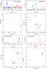 |
Fig. 1 Spectra and maps of 6.7 GHz methanol masers detected using the EVN. The names are the Galactic coordinates of the brightest spots listed in Table 2. The colors of circles relate to the LSR velocities as shown in the spectra. The map origins are the locations of the brightest spots (Table 2). The gray lines show the Torun 32 m dish spectra. If needed, the separate scale of the flux density is presented on the left (EVN) and right (Torun) sides. The thin bars under the spectra show the LSR velocity ranges of spots displayed. The plots for the remaining targets are presented in Appendix A. |
Colors and luminosities of MIR counterparts of methanol and non-methanol sources.
3. Results
A total of 15 maser sources were successfully mapped. Table 2 lists the updated names based on the newly determined positions, the coordinates, the velocity (Vp), and the intensity (Sp) of the brightest spot of each source, the velocity extent of emission (ΔV), as well as the maser extent along the major axis (the longest distance between two maser spots within a given target) and the number of measured spots.
In Figs. 1 and A.1 we present the distribution of the maser emission and the spectrum for each source. The spectra were extracted using the AIPS task ISPEC from the image datacubes using the smallest region covering the entire emission. For two maser sites, W49N and G59.783+00.065, where the emission comes from maser groups separated by more than 0.̋5, but overlaps in velocity, the presented spectra are the sum of the fluxes from all regions. The single-dish spectra are displayed when available.
A maser cloud was defined when the emission in at least three consecutive spectral channels coincides in position within half of the synthesized beam (~2.5 mas). We summarize the numbers and details of clouds with Gaussian velocity profiles for each target in Tables 2 and B.1, respectively. The velocity (Vfit), line width at half maximum (FWHM), and flux density (Sfit) were obtained by fitting a Gaussian profile to the spectrum. The projected length (Lproj) of maser clouds and, if seen, the velocity gradient (Vgrad) are given. The Gaussian velocity profiles are plotted in Fig. A.2.
All the detected maser sources listed in Table 2 coincide within <0.̋5 with MIR counterparts, which are listed in Table 3. As the field of view of EVN observations was about 2.́1 we searched for the maser emission toward other MIR objects, visible in the GLIMPSE maps (Benjamin et al. 2003), lying within a radius of 60′′ of the phase centers (Table 1). No new emission at 6.7 GHz was found within the observed LSR velocity range using the searching method described in Sect. 2.2. The names, Galactic coordinates, 1σ noise levels, velocity range searched for the maser emission, IRAC colors [3.6]−[4.5] and [4.5]−[5.8], and luminosities of MIR counterparts of maser and non-maser objects are given in Table 3. The positions and MIR flux densities are taken from GLIMPSE I Spring ’07 Archive via Gator in the NASA/IPAC Infrared Science Archive. The crowded region of W49N is omitted in Table 3 because of difficulty of identification of discrete sources; all MIR counterparts of the four maser sources are blended and/or saturated. In Table 3 only two MIR objects G40.2819−0.2197 and G45.4725+0.1335 classified as “possible” MYSO outflow candidates in the EGO catalog (Cyganowski et al. 2008) are associated with the maser emission. One object G45.4661+0.0457 listed in Cyganowski et al. as “likely” MYSO outflow candidate has no 6.7 GHz maser emission.
3.1. Individual sources
G37.753−00.189. The weakest source in the sample with a brightest spot of 334 mJy at a velocity of 55.0 km s-1. In total we registered 16 spots, over a velocity range from 54.5 to 65.3 km s-1, grouped into three clusters distributed in a linear structure of length ~150 mas with a clear velocity gradient, redshifted spots in the northeast and blueshifted ones in the southwest. The blue-shifted (54.5−55.0 km s-1) cluster contains two clouds blended in velocity and coinciding in position within ~0.6 mas. Pandian et al. (2011) failed to find any emission using MERLIN in 2007 (they did not notice any emission in the cross-spectra). However, they were successful when using the EVLA in A configuration in 2008; the emission from a compact group of spots with a peak of 2.1 Jy in the velocity range of 54.5−55.1 km s-1 coincides within 20 mas with the EVN position, whereas weaker emission at velocities higher than 60.3 km s-1 is distributed over an area of 150 × 80 mas. This diffuse emission is seen with the EVN as two compact clouds of flux density lower than 0.15 Jy. The integrated flux density obtained with the VLBI is a factor of 4.9 lower than that observed with the 32 m telescope.
G40.282−00.219. This source with 123 maser spots detected between 65.6 km s-1 and 84 km s-1, shows a complex morphology. Fifteen clouds with Gaussian velocity profiles are distributed over an area of 0.̋4 × 0.̋6. We do not notice any overall regularity in the LSR velocities, but 14 out of 15 identified maser clouds showed individual velocity gradients (Table B.1). The source morphology seen with the EVLA by Pandian et al. (2011) is very similar to what we find here, with the exception that they did not map any emission at velocities higher than 79 km s-1 because of the limit of the bandwidth. The shape of the spectrum from the EVN generally agrees with that from the 32 m dish, but the flux density of individual features appears to be reduced by a factor of 1.3−6.7. The features at 65.8 km s-1 and 68.0 km s-1 detected only in the VLBI observation were at the 3σrms noise level in the single-dish spectrum.
G40.425+00.700. The 127 spots detected in the velocity range of 5.2 km s-1 to 16.2 km s-1 delineate an arched structure of a size of 350 mas; 111 of them formed 16 clouds with Gaussian velocity profiles. The strongest and most redshifted (>13.5 km s-1) emission forms the southern cluster of eight clouds distributed over an area of 60 mas. The extreme blueshifted (<8 km s-1) emission is clustered at the northern side of the arch. The source morphology resembles that reported for the ring source G23.657−00.127 (Bartkiewicz et al. 2005). The spectrum obtained with the EVN is very similar to the single-dish spectrum; for two features only the emission is resolved out by ~30−40%. Caswell et al. (2009) reported a velocity range and peak flux similar to ours, but their coordinates differ by 1.̋5 in declination. However, the new position agrees with that obtained by the BeSSeL project3 (Brunthaler et al. 2011).
G41.123−00.220. Two maser clusters are separated by 50 mas and differ in velocity by 8.9 km s-1. The emission near 55.3 km s-1 comes from one eastern cloud, whereas that near 63.4−63.9 km s-1 comes from the western cluster of size ~5 mas. Our map is generally consistent with that obtained with the EVLA (Pandian et al. 2011), but the western cluster appears to contain diffuse emission.
G41.16−00.20. Weak emission was found significantly shifted from the phase center so fringe fitting was applied (Sect. 2.2). Two maser clouds are separated by 50 mas and their velocities differ by 6 km s-1. The source observed with the EVLA shows a complex structure (~100 × 50 mas in extent) of the eastern and redshifted (61.6−63.7 km s-1) emission (Pandian et al. 2011). The flux density recovered with the EVN was about a factor of 2–3 lower than that detected with the EVLA. With this characteristic we can conclude that the VLBI has resolved most of its emission.
G41.226−00.197. Sixty-five spots were detected above 74 mJy in the velocity range of 55.0−63.0 km s-1. They form eight clouds with Gaussian velocity profiles in four clusters. The overall morphology is very similar to that observed with MERLIN (Pandian et al. 2011), with the exception of the two southern redshifted clusters which are more compact. The single-dish spectrum has a similar shape to the MERLIN spectrum, but it is clear that the emission is resolved out by a factor of 2−3 in the EVN observation. The redshifted emission is located in the south, while the blueshifted in the north.
G41.348−00.136. The 66 spots detected in the velocity range from 6.8 km s-1 to 14.7 km s-1 forms nine clouds with Gaussian velocity profiles and are clustered into two groups. The southeastern cluster is blueshifted (<10 km s-1), while the northwestern cluster is redshifted. The two clusters are separated by ~50 mas. The overall morphology of emission agrees well with that obtained with MERLIN (Pandian et al. 2011). For most components the flux density is slightly (0.5−1.0 Jy) reduced compared to the single-dish and MERLIN spectra, but the component near 12 km s-1 is lowered by a factor of two.
W49N. This maser site is of special interest since four sources (Table 2) were detected over an area of 84′′× 55′′ in the velocity range from −1.2 km s-1 to 22.2 km s-1. Two southern sources, G43.149+00.013 and G43.167−00.004, show linear structures (PA = −45°) composed of only ten and four spots, respectively with respective lengths of 4.5 mas and 183 mas. Both sources exhibit a clear velocity gradient. The morphology of G43.149+00.013 agrees well with that observed with MERLIN (Pandian et al. 2011) while the weakest source G43.167−00.004 is largely resolved with the EVN. We note very narrow emission of 0.3 (in the LSR velocity range from −1.25 km s-1 to −0.99 km s-1) and 1.1 km s-1 (from 13.06 km s-1 to 14.11 km s-1) in both sources. The other two sources G43.165+00.013 and G43.171+00.004 are complex with 83 and 36 spots spread over areas of 120 mas × 190 mas and 120 mas × 180 mas, respectively. The velocity extent of emission from G43.165+00.013 is 11.9 km s-1, while that from G43.171+00.004 is 3.4 km s-1. The overall morphologies of these four objects agree with those obtained with MERLIN (Pandian et al. 2011). We did not find any emission from source G43.18−0.01 that was detected in the Arecibo survey (Pandian et al. 2007) and imaged with one spot only (with a flux density of 0.32 mJy) using MERLIN (Pandian et al. 2011). The EVN observation poorly recovered the maser emission from the site; the flux density of individual components are a factor of 3–7 lower that observed with the single dish.
G45.467+00.053. Emission of 4 km s-1 width, composed of 52 spots clustered in eight groups, was detected over an area of 20 mas × 30 mas. The extreme blue- and redshifted emissions delineate two linear structures at PA = − 45° with monotonic velocity gradients. The emission at the intermediate velocity of 57.2−57.9 km s-1 forms a 15 mas linear structure at PA = 90°. Maps obtained with MERLIN show less complex morphology (Pandian et al. 2011). The single-dish spectrum implies that some components at intermediate velocity were resolved out with EVN by a factor of two. No emission near 50 km s-1 was detected in the VLBI data.
G45.473+00.134. Thirty-nine maser spots in the velocity range from 59.5 km s-1 to 66.5 km s-1 form three clusters separated by 0.̋4−1.̋1. The clusters with emission at velocity lower than 64 km s-1 lie 0.̋7 and 0.̋4 to the southwest and to the north, respectively, from the strongest emission near 66 km s-1. The overall morphology is similar to that obtained with MERLIN (Pandian et al. 2011) and the flux density of individual components are only slightly lower than the single-dish spectrum.
G45.493+00.126. The 14 spots detected form a roughly linear structure of size 3 mas with a monotonic velocity gradient of 0.38 km s-1 mas-1 from the west to the east for the blue- and redshifted velocities, respectively. A similar structure was observed with MERLIN (Pandian et al. 2011). The single-dish spectrum indicates that only 50% of the flux was recovered with the EVN for the emission at velocities higher than 57 km s-1.
G59.782+00.065. Two elongated (290 mas and 330 mas) maser clusters separated by 860 mas were detected. The eastern cluster is composed of ten clouds (71 spots) in the velocity range from 15.2 km s-1 to 27.6 km s-1 and the western cluster contains 14 clouds (99 spots) at velocities of 14.3−21.7 km s-1. Almost all maser spots (160/170) form clouds which are fitted by Gaussian profiles. The single-dish spectrum indicates that for most of the components the flux density dropped by ~30% in the EVN observation. There are three features centered at 14.5, 21.5, and 24.5 km s-1 with flux densities which agree within less than 10% of those measured with the single-dish. The 12.2 GHz methanol maser emission of only two features at 17.0 km s-1 and 26.9 km s-1 was reported to form two additional compact clusters of components separated by about 800 mas (Minier et al. 2000).
Sources properties.
4. Discussion
In the subsequent analysis we will consider all the GLIMPSE sources that are listed in Table 3. This allows us to consider sources with and without maser emission, although through the selection we are obviously biased toward maser sources.
4.1. Properties of maser clouds
The kinematic distances to the targets are calculated with recipes of Reid et al. (2009) assuming that the systemic velocity of each individual source is equal to the peak velocity of the 13CO profile (Pandian et al. 2009) or the middle velocity of the maser spectrum (Szymczak et al. 2012). Distance ambiguities have been successfully resolved toward all targets using the 21 cm HI absorption line or the 6 cm formaldehyde absorption line, taken from the literature, and in a few cases the trigonometric distances have been adopted (Table 4).
As we mentioned in Sect. 3, we have calculated the projected length of each identified maser cloud as well as the velocity gradients (Table B.1). Taking the estimated distances we also list these values of the linear scales (Table B.1). In total, we identified 118 maser clouds with Gaussian velocity profiles. Seventeen features were fitted with at least two Gaussian profiles giving 29 additional profiles (e.g., clouds 1, 2, 17 in G40.425+00.700; Table B.1 and Fig. A.2). The projected length of maser clouds ranges from 0.65 AU to 113.32 AU with a mean of 23.61 ± 2.32 AU and a median of 13.96 AU. Velocity gradients of maser clouds show values up to 0.59 km s-1 AU-1, while in some cases no gradients were seen. The mean velocity gradient is 0.051 ± 0.007 km s-1 AU-1 and the median is 0.026 km s-1 AU-1. The FWHM of all 147 (118+29) Gaussian profiles ranged from 0.13 km s-1 to 1.3 km s-1 with a mean of 0.38 ± 0.02 km s-1 and a median of 0.33 km s-1. These values are comparable to those reported from single-dish observations by Pandian & Goldsmith (2007). We do not find a significant difference in median and average values of profile widths between nearby and distant objects.
The luminosity of individual maser clouds was calculated according to the following formula: L6.7 GHz [L⊙] = 6.9129 × 10⁻⁹D2 [kpc] Sint [Jy km s-1]. Its range is 0.33 − 358 × 10-7L⊙ and has a mean of 28.5 ± 4.1 × 10⁻⁷L⊙, and a median of 10.79 × 10⁻⁷L⊙. As one can see the most of the clouds show luminosity below 30 × 10-7L⊙ and a velocity gradient less than 0.15 km s-1 AU-1, but we also note that there is a tendency for the high luminosity (>30 × 10-7L⊙) clouds to have a gradient velocity less than 0.1 km s-1 AU-1 (Fig. 2). This may be related to the direction of the maser filament; the more it is aligned with the line of sight, the less is the velocity gradient seen on the plane of the sky.
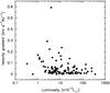 |
Fig. 2 Relationship between the luminosity of a single methanol maser cloud and its velocity gradient (Table B.1). |
4.2. Maser and YSO luminosities
With our sample of maser sources we can attempt to estimate the physical parameters of the central sources since the distances are quite reliably determined. The near- and MIR fluxes for the counterparts of the 11 targets (with the exception of W49N region because of its complexity in the VLBI maps and the lack of IR data at sufficient resolution) were taken from the following publicly available data: UKIDSS-DR6 (Lucas et al. 2008) or 2MASS All−Sky Point Source Catalog (Skrutskie et al. 2006) for G59.782+00.065, Spitzer IRAC (Fazio et al. 2004) and MIPS (Rieke et al. 2004), and MSX (Egan et al. 2003). The far-infrared and sub-millimeter fluxes toward some of the targets were found in the literature; they were taken with SCUBA (Di Francesco et al. 2008), LABOCA and IRAM (Pandian et al. 2010), BOLOCAM (searched for in Rosolowsky et al. 2010 via the VizieR Service and verified with the recent catalog by Ginsburg et al. 2013), Herschel (Veneziani et al. 2013), and SIMBA (Hill et al. 2005). We also made use of the RMS Database Server4 (Urquhart et al. 2008) in order to verify the completeness of found data for some targets. The source infrared fluxes are listed in Table B.2.
Assuming no variability of the infrared emission level, we applied the SED fitter developed by Robitaille et al. (2007) which is based on a grid of SED models spanning a large range of evolutionary stages and stellar masses. They use young stellar objects with various combinations of circumstellar disks, infalling envelopes, and outflow cavities under the assumption that stars form via accretion through the disk and envelope. We set an uncertainty of distance parameter of either 10% or that listed in the literature in a source distance and varied the interstellar extinction, AV, from 0 to 100 magnitudes. Figure 3 shows the model fit of the SED for the first source in our sample, G37.753−00.189. The SEDs of the remaining targets are presented in Fig. A.3. For the sources G40.425+00.700 and G41.16−00.20 the SED fits are poorly constrained because of the lack of far-infrared (>450 μm) flux density measurements. The stellar mass, temperature, radius, total luminosity of the central star, and other properties can be estimated. We found that these parameters for our targets are typical for massive YSOs (De Buizer et al. 2012; Pandian et al. 2010). Here we confine the discussion to the total luminosity, Ltot, which depends on the inclination angle, i, of the model. The range of i is listed in Table 4. We do not include the other properties in the discussion as was done in De Buizer et al. (2012) since they are probably inconclusive. The median, minimum, and maximum values of Ltot from the ten best SED fits based on their χ2 values are calculated for each of the 11 objects (Table 4).
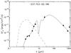 |
Fig. 3 Fit to the spectral energy distribution of the first 6.7 GHz source in the sample. The fits for the remaining targets are presented in Fig. A.3. The filled circles show the input fluxes (Table B.2). The solid line shows the best fit and the gray lines show subsequent good fits. The dashed line shows the stellar photosphere corresponding to the central source in the best fitting model in the absence of circumstellar extinction and in the presence of interstellar extinction. |
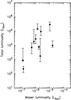 |
Fig. 4 Relationship between the methanol maser luminosity as obtained from the EVN observations and the total luminosity of the central star. The median values of the total luminosity are shown and the vertical bars show the range of the total luminosity. |
We searched for relationships between the total luminosity of the star and the observed properties of the maser emission. The maser (isotropic) luminosity of each target is listed in Table 4 as Lm(EVN). We also give the ratio of the maser luminosity obtained from the EVN observations and single-dish data (Lm(EVN)/Lm(32m)). The average maser luminosity is (3.27 ± 1.28) × 10-6L⊙ and the median value is 1.41 × 10⁻⁶L⊙ (for all 15 targets). These values from the 32 m dish are (14.40 ± 7.85) ×10-6L⊙ and 4.14 ×10⁻⁶L⊙, respectively (for 10 sources).
One can see that the isotropic maser luminosity and the total luminosity show some correlation (Fig. 4). However, we failed to obtain a consistent fit indicating poor statistics (the correlation coefficient shows a very significant uncertainty of 150%). A larger sample (including more distant objects to avoid a bias due to the distance) is needed to verify if the higher maser luminosity is related to higher stellar luminosity. We agree that this relation could put some constraints on the pumping mechanism or indicate that the larger clump/core just provides a longer maser amplification column as pointed out by Urquhart et al. (2013) for analysis of the isotropic maser luminosities and masses of maser-associated submillimetre continuum sources. More luminous central sources would excite larger regions around them and a maser amplification paths would be longer.
4.3. MIR colors and luminosities
The IRAC colors of objects listed in Table 3 do not show statistically significant differences between maser and non-maser sources for our sample (Fig. 5). This appears to be consistent with the survey of 6.7 GHz methanol masers in a sample of 20 MYSO outflow candidates (the EGOs; Cyganowski et al. 2009), where the detection rate was about 64%. Ellingsen (2007) selected a large sample (200) of GLIMPSE sources, likely to be HMSFRs, on the basis of their MIR colors (either bright at 8.0 μm or with extreme [3.6]–[4.5] colors, and devoid of known methanol maser emission) and obtained a 6.7 GHz maser detection rate of about 19%.
The luminosity at 4.5 μm is calculated with the following equation Lν(4.5 μm) [L⊙] = 4.706 × 10⁻³D2 [kpc]Sν(4.5 μm) [mJy]. The flux is taken from the NASA/IPAC Infrared Science Archive via Gator (Sect. 3). Similar equations are used to calculate the luminosities at 3.6 μm and 5.8 μm. It is assumed that the non-maser objects in the field centered at the maser source are members of the same cluster of MYSOs. Median values of Lν(4.5 μm) for maser and non-maser MIR objects are 3.82 L⊙ and 1.12 L⊙, respectively. The same values at IRAC bands 3.6 μm and 5.8 μm are 1.6 (maser MIR), 0.26 (non-maser MIR) and 20.18 (maser MIR), 6.66 L⊙ (non-maser MIR), respectively. We conclude that the likelihood of maser occurrence increases for IR bright objects. This supports a view that the appearance of the maser emission is dependent on the energy output of the central object. Analysis of a larger sample is needed to confirm our result. Moreover, observations at sufficient angular resolution at other wavelengths would help to distinguish whether that effect is related to the evolutionary stage of the central object.
 |
Fig. 5 Color–color diagram of MIR counterparts with methanol emission (black circles) and without (open circles) as listed in Table 3. |
4.4. Maser emission characteristics and origin
There appears to be a correlation of the extent of the maser region with its velocity range (Fig. 6). To obtain more reliable statistics we added measurements from 31 targets from our previous sample (Bartkiewicz et al. 2009). We confirm, as was reported by Pandian et al. (2011), that the larger the emission extent of a maser, the wider its velocity width (a log-log correlation). However, no dependence is clear from the second relation, maser luminosity vs. emission extent (Fig. 6). In the plot we highlight seven masers with clear ring-like morphology (six from Bartkiewicz et al. 2009 that consist of more than four groups of maser spots, the obvious fitting of an ellipse, and the G40.425+00.700 source from this sample). They all tend to fall in a region with higher emission extent (>330 AU) and velocity width (>4.8 km s-1). The ring-like 6.7 GHz methanol maser discovered toward Cep A has similar properties with the extent of 960 AU and ΔV = 3.2 km s-1 (Sugiyama et al. 2008; Torstensson et al. 2011). Three new methanol maser rings (with more than four groups of maser spots) have been detected recently by Fujisawa et al. (2014) toward 000.54−00.85 SE, 002.53+00.19, and 025.82−00.17. They also showed the high linear extent (1500–4500 AU) and significant velocity width (ΔV from 8.8 km s-1 to 16 km s-1).
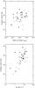 |
Fig. 6 Top: relationship between the isotropic maser luminosity as obtained from the EVN data and its spatial extent (the major axis) and bottom: relationship between the velocity extent of the methanol maser line and the spatial extent. The targets from this paper are marked with black circles; the targets from Bartkiewicz et al. (2009) are marked with open circles and triangles (the sources with clear ring-like morphology containing more than four maser spot groups). |
Comparison of the methanol maser profiles taken from the EVN and single-dish observations reveals that about 57% of the maser flux density is resolved out (Table 4). The fraction of missing flux ranges from 24% in G40.425+00.700 to 86% in G37.753−00.189. Its value clearly does not depend on the distance of the source which implies that the occurrence of weak and diffuse maser emission is specific to an individual source. The lack of information on the distribution of weak and diffuse emission may prevent the determination of the full extent and morphology of the maser source. We note that 12 sources in the sample were observed with the EVLA and/or MERLIN with beamsizes of 0.̋45 × 0.̋26 and 0.̋060 × 0.̋035, respectively (Pandian et al. 2010). The overall morphologies of these sources obtained with the VLBI agree well with those observed with lower angular resolution. This implies that almost all maser clouds have compact cores and the source structures are actually recovered.
All the maser targets are usually associated with the brightest MYSOs within each cluster showing an excess of extended 4.5 μm emission. However, only two of the eleven maser sources (Table 3) are associated with “possible” MYSO outflow candidates in the EGO catalog (Cyganowski et al. 2008). We note that these sources G40.2819−0.2197 and G45.4725+0.1335 are in a group of objects with the linear projected size of maser emission greater than 2700 AU (Table 2). Therefore, the maser emission may arise in outflows or in multiple nearby point sources. The source G45.4661+0.0457 reported by Cyganowski et al. (2008) as a “likely” MYSO outflow candidate is a non-maser source. They estimated a lower limit of detection rate of 6.7 GHz maser emission in “likely” MYSO outflow candidate EGOs as high as 73%. We can conclude that in our sample the maser emission is rarely associated with outflows traced by extended 4.5 μm emission. Most of our maser sources are associated with the MIR objects easily identified via color selection in the GLIMPSE I Spring 07 Archive (Table 3). The appearance of their 4.5 μm emission excess of angular extents from a few to less than 10′′ could be related to high extinction (Rathborne et al. 2005; Cyganowski et al. 2008). This implies that most of our masers are associated with highly embedded MYSOs. Coarse angular resolution MIR images cannot be easily compared with the VLBI images of mas resolution to examine whether the maser arises in outflows or in disks. It seems that the proper motion studies of maser components is only one way to verify the ongoing phenomenon.
5. Conclusions
We successfully imaged the 6.7 GHz methanol emission toward 15 targets (four of them belong to the complex HMSFR W49N). Using a short correlation time (0.25 s) we were able to image significantly offset emission of −54′′ in RA and −56′′ in Dec (G43.149+00.013) from the pointing center. Although the VLBI resolves some of the emission, there is no problem studying the morphology; almost all maser clouds must have compact cores. The maser emission was always associated with the strongest MIR counterpart in the clusters, so we conclude that the appearance of the maser emission is related to the IR brightness of the central MYSO. The maser (isotropic) luminosity and the total luminosity of the central object are likely to correlate; however, a larger sample is needed to verify this relation. The maser linear extent is related to its spectrum width. We also note that the spectra of methanol rings are the widest among the sample and their emission also appears more extended on the sky.
Online material
Appendix A: Figures
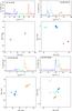 |
Fig. A.1 Spectra and maps of 6.7 GHz methanol masers detected using the EVN. The names are the Galactic coordinates of the brightest spots listed in Table 2. The colors of circles relate to the LSR velocities as shown in the spectra. The map origins are the locations of the brightest spots (Table 2). The gray lines show the Torun 32 m dish spectra. If needed, the separate scale of the flux density is presented on the left (EVN) and right (Torun) sides. The thin bars under the spectra show the LSR velocity ranges of spots displayed. The plots for the first four targets are presented in Fig. 1. |
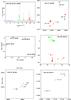 |
Fig. A.1 continued. For clarity, in G43.171+00.004, G43.167−0.004, and G43.149+0.013, we listed the LSR velocities in km s-1 (or LSR velocity range) of a given maser (or maser groups). |
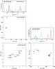 |
Fig. A.1 continued. In G45.493+00.126 we listed the LSR velocities in km s-1 (or LSR velocity range) of a given maser (or maser groups). |
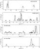 |
Fig. A.2 Spectra of individual 6.7 GHz maser clouds with Gaussian velocity profiles. Each circle traces the emission level of a single maser spot as presented in Figs. 1 and A.1. The black line represents the fitting of a Gaussian function (or functions) as summarized in Table B.1. The gray line presents the single Gaussian fitting in a case of complex velocity profile of an individual component. |
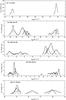 |
Fig. A.2 continued. |
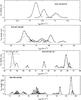 |
Fig. A.2 continued. |
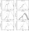 |
Fig. A.3 Fit to the spectral energy distribution for the remaining targets. |
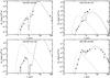 |
Fig. A.3 continued. |
Appendix B: Tables
Parameters of 6.7 GHz methanol maser clouds with Gaussian velocity profiles.
Auxiliary inputs to the SED models.
Acknowledgments
A.B. and M.S. acknowledge support from the National Science Centre Poland through grant 2011/03/B/ST9/00627. We thank Dr Jagadheep Pandian for useful discussions. We thank the referee for a detailed and constructive report which improved this article. This work has also been supported by the European Community Framework Programme 7, Advanced Radio Astronomy in Europe, grant agreement No. 227290. This research has made use of the VizieR catalog access tool, CDS, Strasbourg, France. This research made use of data products from the Midcourse Space Experiment. This research has also made use of the NASA/ IPAC Infrared Science Archive at http://irsa.ipac.caltech.edu/, which is operated by the Jet Propulsion Laboratory, California Institute of Technology, under contract with NASA. This paper made use of information from the Red MSX Source survey database at www.ast.leeds.ac.uk/RMS which was constructed with support from the Science and Technology Facilities Council of the UK.
References
- Bartkiewicz, A., Szymczak, M., & van Langevelde, H. J. 2005, A&A, 442, L61 [NASA ADS] [CrossRef] [EDP Sciences] [Google Scholar]
- Bartkiewicz, A., Szymczak, M., van Langevelde, H. J., Richards, A. M. S., & Pihlström, Y. M. 2009, A&A, 502, 155 [NASA ADS] [CrossRef] [EDP Sciences] [Google Scholar]
- Benjamin, R. A., Churchwell, E., Babler, B. L., et al. 2003, PASP, 115, 953 [NASA ADS] [CrossRef] [Google Scholar]
- Brunthaler, A., Reid, M. J., Menten, K. M., et al. 2011, Astron. Nachr., 332, 461 [NASA ADS] [CrossRef] [Google Scholar]
- Caswell, J. L. 2009, PASA, 26, 454 [NASA ADS] [CrossRef] [Google Scholar]
- Chambers, E. T., Jackson, J. M., Rathborne, J. M., & Simon, R. 2009, ApJS, 181, 360 [NASA ADS] [CrossRef] [Google Scholar]
- Cyganowski, C. J., Whitney, B. A., Holden, E., et al. 2008, AJ, 136, 2391 [NASA ADS] [CrossRef] [Google Scholar]
- Cyganowski, C. J., Brogan, C. L., Hunter, T. R., & Churchwell, E. 2009, ApJ, 702, 1615 [NASA ADS] [CrossRef] [Google Scholar]
- De Buizer, J. M., & Vacca, W. D. 2010, AJ, 140, 196 [NASA ADS] [CrossRef] [Google Scholar]
- De Buizer, J. M., Bartkiewicz, A., & Szymczak, M. 2012, ApJ, 754, 149 [NASA ADS] [CrossRef] [Google Scholar]
- Di Francesco, J., Johnstone, D., Kirk, H., et al. 2008, ApJS, 175, 277 [NASA ADS] [CrossRef] [Google Scholar]
- Dodson, R., Ojha, R., & Ellingsen, S. P. 2004, MNRAS, 351, 779 [NASA ADS] [CrossRef] [Google Scholar]
- Egan, M. P., Price, S. D., & Kraemer, K. E. 2003, Am. Astron. Soc. Meet., 203, # 57.08, BAAS, 35, 1301 [NASA ADS] [Google Scholar]
- Ellingsen, S. P. 2007, MNRAS, 377, 571 [NASA ADS] [CrossRef] [Google Scholar]
- Fazio, G. G., Hora, J. L., Allen, L. E., et al. 2004, ApJS, 154, 10 [NASA ADS] [CrossRef] [Google Scholar]
- Fujisawa, K., Sugiyama, K., Motogi, K., et al. 2014, PASJ, 66, 2 [Google Scholar]
- Ginsburg, A., Glenn, J., Rosolowsky, E., et al. 2013, ApJS, 208, 14 [NASA ADS] [CrossRef] [MathSciNet] [Google Scholar]
- Goddi, C., Moscadelli, L., & Sanna, A. 2011, A&A, 535, L8 [NASA ADS] [CrossRef] [EDP Sciences] [Google Scholar]
- Hill, T., Burton, M. G., Minier, V., et al. 2005, MNRAS, 363, 405 [NASA ADS] [CrossRef] [Google Scholar]
- Lucas, P. W., Hoare, M. G., Longmore, A., et al. 2008, MNRAS, 391, 136 [NASA ADS] [CrossRef] [Google Scholar]
- Menten, K. M. 1991, ApJ, 380, L75 [NASA ADS] [CrossRef] [Google Scholar]
- Minier, V., Booth, R. S., & Conway, J. E. 2000, A&A, 362, 1093 [NASA ADS] [Google Scholar]
- Moscadelli, L., Cesaroni, R., Rioja, M. J., Dodson, R., & Reid, M. J. 2011, A&A, 526, A66 [NASA ADS] [CrossRef] [EDP Sciences] [Google Scholar]
- Norris, R. P., Byleveld, S. E., Diamond, P. J., et al. 1998, ApJ, 508, 275 [NASA ADS] [CrossRef] [Google Scholar]
- Pandian, J. D., & Goldsmith, P. F. 2007, ApJ, 669, 435 [NASA ADS] [CrossRef] [Google Scholar]
- Pandian, J. D., Goldsmith, P. F., & Deshpande, A. A. 2007, ApJ, 656, 255 [NASA ADS] [CrossRef] [Google Scholar]
- Pandian, J. D., Menten, K. M., & Goldsmith, P. F. 2009, ApJ, 706, 1609 [NASA ADS] [CrossRef] [Google Scholar]
- Pandian, J. D., Momjian, E., Xu, Y., Menten, K. M., & Goldsmith, P. F. 2010, A&A, 522, A8 [NASA ADS] [CrossRef] [EDP Sciences] [Google Scholar]
- Pandian, J. D., Momjian, E., Xu, Y., Menten, K. M., & Goldsmith, P. F. 2011, ApJ, 730, 55 [NASA ADS] [CrossRef] [Google Scholar]
- Rathborne, J. M., Jackson, J. M., Chambers, E. T., et al. 2005, ApJ, 630, L181 [NASA ADS] [CrossRef] [Google Scholar]
- Reid, M. J., Menten, K. M., Zheng, X. W., et al. 2009, ApJ, 700, 13 [NASA ADS] [Google Scholar]
- Rieke, G. H., Young, E. T., Engelbracht, C. W., et al. 2004, ApJS, 154, 25 [NASA ADS] [CrossRef] [Google Scholar]
- Robitaille, T. P., Whitney, B. A., Indebetouw, R., & Wood, K. 2007, ApJS, 169, 328 [NASA ADS] [CrossRef] [Google Scholar]
- Rosolowsky, E., Dunham, M. K., Ginsburg, A., et al. 2010, ApJS, 188, 123 [NASA ADS] [CrossRef] [Google Scholar]
- Sanna, A., Moscadelli, L., Cesaroni, R., et al. 2010a, A&A, 517, A71 [NASA ADS] [CrossRef] [EDP Sciences] [Google Scholar]
- Sanna, A., Moscadelli, L., Cesaroni, R., et al. 2010b, A&A, 517, A78 [NASA ADS] [CrossRef] [EDP Sciences] [Google Scholar]
- Skrutskie, M. F., Cutri, R. M., Stiening, R., et al. 2006, AJ, 131, 1163 [NASA ADS] [CrossRef] [Google Scholar]
- Sugiyama, K., Fujisawa, K., Doi, A., et al. 2008, PASJ, 60, 23 [NASA ADS] [Google Scholar]
- Szymczak, M., Wolak, P., Bartkiewicz, A., & Borkowski, K. M. 2012, Astron. Nachr., 333, 634 [NASA ADS] [CrossRef] [Google Scholar]
- Torstensson, K. J. E., van Langevelde, H. J., Vlemmings, W. H. T., & Bourke, S. 2011, A&A, 526, A38 [NASA ADS] [CrossRef] [EDP Sciences] [Google Scholar]
- Urquhart, J. S., Hoare, M. G., Lumsden, S. L., Oudmaijer, R. D., & Moore, T. J. T. 2008, ASP Conf. Ser., 387,381 [NASA ADS] [Google Scholar]
- Urquhart, J. S., Moore, T. J. T., Schuller, F., et al. 2013, MNRAS, 431, 1752 [Google Scholar]
- Veneziani, M., Elia, D., Noriega-Crespo, A., et al. 2013, A&A, 549, A130 [NASA ADS] [CrossRef] [EDP Sciences] [Google Scholar]
- Watson, C., Araya, E., Sewilo, M., et al. 2003, ApJ, 587, 714 [NASA ADS] [CrossRef] [Google Scholar]
- Xu, Y., Reid, M. J., Menten, K. M., et al. 2009, ApJ, 693, 413 [NASA ADS] [CrossRef] [Google Scholar]
- Zhang, B., Reid, M. J., Menten, K. M., et al. 2013, ApJ, 775, 79 [NASA ADS] [CrossRef] [Google Scholar]
All Tables
Colors and luminosities of MIR counterparts of methanol and non-methanol sources.
All Figures
|
Fig. 1 Spectra and maps of 6.7 GHz methanol masers detected using the EVN. The names are the Galactic coordinates of the brightest spots listed in Table 2. The colors of circles relate to the LSR velocities as shown in the spectra. The map origins are the locations of the brightest spots (Table 2). The gray lines show the Torun 32 m dish spectra. If needed, the separate scale of the flux density is presented on the left (EVN) and right (Torun) sides. The thin bars under the spectra show the LSR velocity ranges of spots displayed. The plots for the remaining targets are presented in Appendix A. |
| In the text | |
|
Fig. 2 Relationship between the luminosity of a single methanol maser cloud and its velocity gradient (Table B.1). |
| In the text | |
|
Fig. 3 Fit to the spectral energy distribution of the first 6.7 GHz source in the sample. The fits for the remaining targets are presented in Fig. A.3. The filled circles show the input fluxes (Table B.2). The solid line shows the best fit and the gray lines show subsequent good fits. The dashed line shows the stellar photosphere corresponding to the central source in the best fitting model in the absence of circumstellar extinction and in the presence of interstellar extinction. |
| In the text | |
|
Fig. 4 Relationship between the methanol maser luminosity as obtained from the EVN observations and the total luminosity of the central star. The median values of the total luminosity are shown and the vertical bars show the range of the total luminosity. |
| In the text | |
|
Fig. 5 Color–color diagram of MIR counterparts with methanol emission (black circles) and without (open circles) as listed in Table 3. |
| In the text | |
|
Fig. 6 Top: relationship between the isotropic maser luminosity as obtained from the EVN data and its spatial extent (the major axis) and bottom: relationship between the velocity extent of the methanol maser line and the spatial extent. The targets from this paper are marked with black circles; the targets from Bartkiewicz et al. (2009) are marked with open circles and triangles (the sources with clear ring-like morphology containing more than four maser spot groups). |
| In the text | |
|
Fig. A.1 Spectra and maps of 6.7 GHz methanol masers detected using the EVN. The names are the Galactic coordinates of the brightest spots listed in Table 2. The colors of circles relate to the LSR velocities as shown in the spectra. The map origins are the locations of the brightest spots (Table 2). The gray lines show the Torun 32 m dish spectra. If needed, the separate scale of the flux density is presented on the left (EVN) and right (Torun) sides. The thin bars under the spectra show the LSR velocity ranges of spots displayed. The plots for the first four targets are presented in Fig. 1. |
| In the text | |
|
Fig. A.1 continued. For clarity, in G43.171+00.004, G43.167−0.004, and G43.149+0.013, we listed the LSR velocities in km s-1 (or LSR velocity range) of a given maser (or maser groups). |
| In the text | |
|
Fig. A.1 continued. In G45.493+00.126 we listed the LSR velocities in km s-1 (or LSR velocity range) of a given maser (or maser groups). |
| In the text | |
|
Fig. A.2 Spectra of individual 6.7 GHz maser clouds with Gaussian velocity profiles. Each circle traces the emission level of a single maser spot as presented in Figs. 1 and A.1. The black line represents the fitting of a Gaussian function (or functions) as summarized in Table B.1. The gray line presents the single Gaussian fitting in a case of complex velocity profile of an individual component. |
| In the text | |
|
Fig. A.2 continued. |
| In the text | |
|
Fig. A.2 continued. |
| In the text | |
|
Fig. A.3 Fit to the spectral energy distribution for the remaining targets. |
| In the text | |
|
Fig. A.3 continued. |
| In the text | |
Current usage metrics show cumulative count of Article Views (full-text article views including HTML views, PDF and ePub downloads, according to the available data) and Abstracts Views on Vision4Press platform.
Data correspond to usage on the plateform after 2015. The current usage metrics is available 48-96 hours after online publication and is updated daily on week days.
Initial download of the metrics may take a while.