| Issue |
A&A
Volume 564, April 2014
|
|
|---|---|---|
| Article Number | A77 | |
| Number of page(s) | 16 | |
| Section | Astrophysical processes | |
| DOI | https://doi.org/10.1051/0004-6361/201322520 | |
| Published online | 10 April 2014 | |
Simulations of gamma-ray burst afterglows with a relativistic kinetic code
1
Astronomy Division, Department of Physics,
PO Box 3000, 90014 University of Oulu, Finland
e-mail:
This email address is being protected from spambots. You need JavaScript enabled to view it.
, This email address is being protected from spambots. You need JavaScript enabled to view it.
2
Physics Department and Columbia Astrophysics Laboratory, Columbia
University, 538 West 120th
Street, New York,
NY
10027,
USA
3
Tartu Observatory, 61602
Tõravere, Tartumaa, Estonia
e-mail:
This email address is being protected from spambots. You need JavaScript enabled to view it.
4
Tuorla Observatory, University of Turku,
Väisäläntie 20,
21500
Piikkiö,
Finland
Received:
21
August
2013
Accepted:
16
February
2014
Abstract
Aims. This paper introduces a kinetic code that simulates gamma-ray burst (GRB) afterglow emission from the external forward shock and presents examples of some of its applications. One interesting research topic discussed in the paper is the high-energy radiation produced by Compton scattering of the prompt GRB photons against the shock-accelerated electrons. The difference between the forward shock emission in a wind-type and a constant-density medium is also studied, and the emission due to Maxwellian electron injection is compared to the case with pure power-law electrons.
Methods. The code calculates the time-evolving photon and electron distributions in the emission region by solving the relativistic kinetic equations for each particle species. For the first time, the full relativistic equations for synchrotron emission/absorption, Compton scattering, and pair production/annihilation were applied to model the forward shock emission. The synchrotron self-absorption thermalization mechanism, which shapes the low-energy end of the electron distribution, was also included in the electron equation.
Results. The simulation results indicate that inverse Compton scattering of the prompt GRB photons can produce a luminous ≳TeV emission component, even when pair production in the emission region is taken into account. This very high-energy radiation may be observable in low-redshift GRBs. The test simulations also show that the low-energy end of a pure power-law distribution of electrons can thermalize owing to synchrotron self-absorption in a wind-type environment, but without an observable impact on the radiation spectrum. Moreover, a flattening in the forward shock X-ray light curve may be expected when the electron injection function is assumed to be purely Maxwellian instead of a power law. The flux during such a flattening is likely to be lower than the Swift/XRT sensitivity in the case of a constant-density external medium, but a wind environment may result in a higher flux during the shallow decay.
Key words: gamma-ray burst: general / radiation mechanisms: non-thermal / methods: numerical
© ESO, 2014
1. Introduction
Gamma-ray burst (GRB) afterglows are produced by relativistic electrons radiating mainly via the synchrotron and inverse Compton mechanisms. According to the standard afterglow model, the electrons are accelerated to highly relativistic energies at two shock fronts, the forward shock and the reverse shock, which are the result of the interaction between the relativistic jet from the GRB central engine and the surrounding medium (for reviews, see, e.g., Piran 2004; Mészáros 2006).
The earliest afterglow models invoke pure synchrotron radiation from the forward shock in a constant-density interstellar medium (ISM) or a wind-type environment and yield analytic time-evolving synchrotron spectra of the decelerating blast wave (Sari et al. 1998; Chevalier & Li 2000; Granot & Sari 2002). The role of inverse Compton scattering of the synchrotron photons has also been investigated, typically relying on an approximate treatment of the scattering process because no analytic solution for the inverse Compton spectrum is available (Panaitescu & Meszaros 1998; Chiang & Dermer 1999; Panaitescu & Kumar 2000; Sari & Esin 2001).
The GRB observations by the Swift and Fermi satellites have revealed some surprising features in the afterglow and prompt light curves, resulting in a need to improve the models for GRB emission. For example, the Fermi/LAT telescope has observed >100 MeV emission from several GRBs. In the literature, the high-energy radiation has been attributed to the prompt emission (e.g., Abdo et al. 2009), to pure synchrotron radiation from the external shock (Gao et al. 2009; Ghisellini et al. 2010; Kumar & Barniol Duran 2010), to a combination of external synchrotron photons and synchrotron self-Compton emission (Tam et al. 2013; Wang et al. 2013; Liu et al. 2013; Fan et al. 2013), and to a superposition of the prompt and afterglow emission (Maxham et al. 2011). Another possibility is that some of the high-energy emission stems from prompt photons being Compton scattered to higher energies by the afterglow-emitting electrons (Beloborodov 2005b; He et al. 2012; Beloborodov et al. 2013; Fan et al. 2013).
Owing to the Swift observations, it has been discovered that a typical X-ray light curve begins with a phase of steeply decaying flux, which is often followed by a shallow decay segment. The late-time afterglow, on the other hand, can often be explained by the standard synchrotron model (Granot & Kumar 2006; Fan & Piran 2006). Energy injection to the blast wave is currently the most popular explanation for the shallow decay phase observed both in X-ray and optical afterglows (Granot & Kumar 2006; Fan & Piran 2006; Nousek et al. 2006; Zhang et al. 2006; Panaitescu & Vestrand 2011; Li et al. 2012). Other models introduced to explain the shallow decay phase include the evolution of microphysical parameters (Panaitescu et al. 2006; Granot et al. 2006), emission due to an outflow ejected before the prompt GRB (Yamazaki 2009; Birnbaum et al. 2012), an off-axis viewing angle of the jet (Eichler & Granot 2006), dust scattering of X-rays (Shao & Dai 2007), late prompt emission (Ghisellini et al. 2007; Murase et al. 2011), and an adiabatic evolution of the shock following a radiative phase (Dermer 2007). It has also been suggested that the main contribution to the afterglow could come from a long-lived reverse shock, which may also explain the shallow decay phase in the X-ray afterglows (Uhm & Beloborodov 2007; Genet et al. 2007).
Models aiming to explain all the different slopes seen in the light curves have also been presented, including accretion of different layers of the progenitor star (Kumar et al. 2008) and the curvature effect that is usually only invoked to explain the early steep X-ray decay (Qin 2008).
The evolution of the GRB blast wave is described well by the self-similar solution by Blandford & McKee (1976), which is valid in the deceleration phase while the blast is still highly relativistic. The evolution in the late non-relativistic phase is given by the Sedov-Taylor solution (Sedov 1959; Taylor 1950). A mechanical model of the relativistic blast ensuring mass, energy, and momentum conservation has been presented by Beloborodov & Uhm (2006), and it is nearly identical to the Blandford-McKee solution at late times after the shock has started to decelerate. However, the mechanical model gives an accurate description of the blast also before the deceleration time, while earlier models unphysically assume an equal pressure at the forward and reverse shock. The evolution of the shell in the mildly relativistic phase can be found by means of hydrodynamic simulations, which can then be coupled to a radiation code to find the radiation spectrum from the shock. Such simulations can also be applied to calculate the afterglow emission for an observer with an off-axis viewing angle (van Eerten et al. 2010a).
Results of one- and two-dimensional hydrodynamic simulations of the blast wave have been presented by Kobayashi et al. (1999), Meliani et al. (2007), Mimica et al. (2009), and Ramirez-Ruiz & MacFadyen (2010) but without discussing the radiation mechanism of the afterglow. A calculation of the synchrotron radiation from the blast has been coupled to the hydrodynamic simulations of Downes et al. (2002), Zhang & MacFadyen (2009), van Eerten et al. (2010b, 2011), and Wygoda et al. (2011). However, none of these works calculate the afterglow component due to Compton scattering, which is expected to appear at high energies.
Simulations including an accurate treatment of both synchrotron and Compton processes, as well as pair production, have been presented by Petropoulou & Mastichiadis (2009) (PM09), who use the solution of Blandford & McKee (1976) to evaluate the evolution of the emitting shell. The code developed by PM09 is similar to the one presented in this paper, but it does not account for the electron heating due to synchrotron self-absorption.
For the first time, we present simulations of afterglow emission from the forward shock with a relativistic kinetic code that treats synchrotron emission and absorption, Compton scattering, and electron-positron pair production/annihilation in a self-consistent way. The kinetic equations determining the time evolution of the electron and photon distributions are solved simultaneously at each timestep. We also consider electron heating due to synchrotron self-absorption, which shapes the electron distribution at low energies.
Our treatment accounts for the fact that electrons injected at different times also have different cooling histories. For example, the magnetic field that determines the synchrotron cooling rate evolves while the electrons are cooling. It follows that there are no sharp cooling breaks in the electron distribution (Uhm & Zhang 2014).
The current version of the code applies a one-zone model of the emission region. It does not account for the different locations of the particles behind the shock and assumes a constant magnetic field throughout the shell. A more accurate treatment of synchrotron emission would require a model of the magnetic field structure behind the shock. Also, knowledge of the spatial photon and electron distributions is required for an exact calculation of Compton scattering.
As an example of the applications of the code, we report the results of a simulation where the afterglow-emitting electrons interact with an external source of photons roughly corresponding to prompt GRB emission. The shocked electrons are expected to upscatter a small fraction of the prompt photons to GeV−TeV energies as long as the prompt emission overlaps with the shocked electrons (Beloborodov 2005b; Fan et al. 2005). Some of the high-energy photons then produce pairs with the prompt MeV photons, which in turn are able to scatter radiation to higher energies.
In addition, we compare the forward shock emission in a wind environment with the emission in a constant-density ISM. The results indicate that a power-law electron distribution can thermalize at low energies thanks to synchrotron self-absorption heating in a wind medium with a typical density structure expected from the surroundings of a Wolf-Rayet star. Along with the ambient density, the importance of thermalization is mainly determined by the fraction of shock-generated energy given to the magnetic field. Our simulations imply that the thermalized electrons are unlikely to produce an observable signature in the afterglow spectrum.
In our final example, we study the difference between the forward shock radiation due to Maxwellian and power-law electron injection. The standard afterglow model assumes that the injection function is a pure power law, even though a large fraction of the shock-generated energy goes to a thermal population of electrons. We find that pure Maxwellian injection can lead to a flattening in the X-ray light curve. The flux during this phase is found to be very low compared to Swift/XRT detections for a constant-density ISM, but detectable flux levels during the shallow decay may be achieved in a wind-type environment.
2. Physical model of the afterglow
2.1. Hydrodynamic evolution
The relativistic shell ejected by the GRB central engine initially propagates into the
surrounding medium with a constant Lorentz factor Γ0. After sweeping an external
mass M0/Γ0,
where M0 is the initial mass of the ejecta, the
shell starts to decelerate according to a self-similar solution found by Blandford & McKee (1976). The self-similar
solution is no longer valid if the reverse shock is long-lived (Uhm et al. 2012) or if there is significant lateral spreading of the
shell after the jet break time (Rhoads 1999). In
the rest of the paper, except for Sects. 3.1 and
3.3, the quantities measured in the fluid comoving
frame are indicated by primes and the unprimed quantities are given in the observer frame.
However, the electron Lorentz factor γ and dimensionless momentum  (1)along with the electron
number density per unit energy (N(γ)) or momentum (N(p))
interval, are always expressed in the fluid frame but left unprimed to simplify the
notation. In the following, we assume an adiabatic hydrodynamic evolution of the blast
wave, which means negligible radiation losses. This assumption is valid even if the
electrons cool rapidly as long as the main fraction of the shock-generated energy is given
to the protons, which do not radiate efficiently.
(1)along with the electron
number density per unit energy (N(γ)) or momentum (N(p))
interval, are always expressed in the fluid frame but left unprimed to simplify the
notation. In the following, we assume an adiabatic hydrodynamic evolution of the blast
wave, which means negligible radiation losses. This assumption is valid even if the
electrons cool rapidly as long as the main fraction of the shock-generated energy is given
to the protons, which do not radiate efficiently.
The bulk Lorentz factor of the shocked fluid evolves with radius r approximately as
 (2)where the value of the
index g
depends on the structure of the ambient medium. If the medium has a constant density,
(2)where the value of the
index g
depends on the structure of the ambient medium. If the medium has a constant density,
 (3)where
RB ≡
Rdec/22/3 is the approximate radius at which the Lorentz factor starts to
decrease from its initial value Γ0, and Rdec is the so-called deceleration
radius, i.e., the radius where the shell has lost half of its initial kinetic energy and
Γ = Γ0/2 (Rees & Meszaros
1992). According to this definition,
(3)where
RB ≡
Rdec/22/3 is the approximate radius at which the Lorentz factor starts to
decrease from its initial value Γ0, and Rdec is the so-called deceleration
radius, i.e., the radius where the shell has lost half of its initial kinetic energy and
Γ = Γ0/2 (Rees & Meszaros
1992). According to this definition,  (4)where
E0 is the isotropic equivalent energy of
the blast wave after the prompt GRB emission, and n0 the electron
number density of the external medium.
(4)where
E0 is the isotropic equivalent energy of
the blast wave after the prompt GRB emission, and n0 the electron
number density of the external medium.
In the case of a wind-type medium with a density profile n(r) =
Awr-2, where
Aw is a constant giving the number of
particles per unit length,  (5)where
RB ≡
Rdec/4, and
(5)where
RB ≡
Rdec/4, and
 (6)The shock radius and the
Lorentz factor of the shocked ejecta are related to the fluid comoving time
t′ according to
(6)The shock radius and the
Lorentz factor of the shocked ejecta are related to the fluid comoving time
t′ according to  (7)and the observed
time can be obtained from
(7)and the observed
time can be obtained from  (8)where
z is the
redshift of the GRB. Before the deceleration time, i.e., r<Rdec,
(8)where
z is the
redshift of the GRB. Before the deceleration time, i.e., r<Rdec,
 (9)For
r ≫
Rdec, the radius evolves in time as
(9)For
r ≫
Rdec, the radius evolves in time as
![Mathematical equation: \begin{eqnarray} \label{eq:r_time} r = \left\{ \begin{array}{ll} \left[3 E_0 t/(2\pi n_0 \mpr c (1+z))\right]^{1/4} & \textrm{(ISM)} \\[3mm] \left[E_0 t/(4\pi \Aw \mpr c (1+z))\right]^{1/2} & \textrm{(wind)} \end{array} \right. \end{eqnarray}](/articles/aa/full_html/2014/04/aa22520-13/aa22520-13-eq35.png) (10)and
the bulk Lorentz factor evolves as
(10)and
the bulk Lorentz factor evolves as ![Mathematical equation: \begin{eqnarray} \label{eq:g_time} \Gamma = \left\{ \begin{array}{ll} \left[3 E_0 (1+z)^3/(2^{13}\pi n_0 \mpr c^5 t^3)\right]^{1/8} & \textrm{(ISM)} \\[3mm] \left[E_0 (1+z)/(64\pi \Aw \mpr c^3 t)\right]^{1/4} & \textrm{(wind)}. \end{array} \right. \end{eqnarray}](/articles/aa/full_html/2014/04/aa22520-13/aa22520-13-eq36.png) (11)One
of the main uncertainties of the afterglow model is the strength of the magnetic field in
the emission region. We adopt the typical approach to the problem and assume that a
fraction ϵB of the
shock-generated energy goes into the energy of the shock-compressed interstellar magnetic
field. The comoving magnetic field B′ then evolves in the emission region
with Γ and n as
(11)One
of the main uncertainties of the afterglow model is the strength of the magnetic field in
the emission region. We adopt the typical approach to the problem and assume that a
fraction ϵB of the
shock-generated energy goes into the energy of the shock-compressed interstellar magnetic
field. The comoving magnetic field B′ then evolves in the emission region
with Γ and n as  (12)determined from the shock
jump conditions (Blandford & McKee 1976).
(12)determined from the shock
jump conditions (Blandford & McKee 1976).
2.2. Distribution of the accelerated electrons
The forward and reverse shocks are thought to be capable of accelerating electrons to
relativistic energies according to a power-law distribution (e.g., Achterberg et al. 2001) of the form  (13)for
γmin ≤
γ ≤ γmax, where
s is the
power-law index, and γ the random Lorentz factor of an electron measured
in the fluid frame. However, simulations by Spitkovsky
(2008) and Martins et al. (2009) show that
shock acceleration actually leads to a hybrid distribution with low-energy Maxwellian
electrons connected to a high-energy power-law tail. An afterglow model that assumes such
a distribution is discussed by Giannios &
Spitkovsky (2009).
(13)for
γmin ≤
γ ≤ γmax, where
s is the
power-law index, and γ the random Lorentz factor of an electron measured
in the fluid frame. However, simulations by Spitkovsky
(2008) and Martins et al. (2009) show that
shock acceleration actually leads to a hybrid distribution with low-energy Maxwellian
electrons connected to a high-energy power-law tail. An afterglow model that assumes such
a distribution is discussed by Giannios &
Spitkovsky (2009).
The number of electrons injected at a shock per unit time is obtained by multiplying the
number density of electrons in the downstream frame, Γn, by the volume swept by
the shock per unit time, 4πr2βc.
Dividing this quantity by the volume of the shell, 4πr2ΔR′,
one finds that the number of injected electrons per unit time and volume is  (14)Assuming a pure power-law
distribution, the minimum Lorentz factor determined from the shock jump conditions (Sari et al. 1996) is
(14)Assuming a pure power-law
distribution, the minimum Lorentz factor determined from the shock jump conditions (Sari et al. 1996) is  (15)where ϵe is the
fraction of the shock-generated energy given to the electrons. This relation holds for
γmin ≪
γmax.
(15)where ϵe is the
fraction of the shock-generated energy given to the electrons. This relation holds for
γmin ≪
γmax.
The maximum Lorentz factor γmax is determined either by the radiation losses of the electrons, the age of the flow, or the saturation limit discussed by Sironi et al. (2013), among others. Typically it has been assumed that the value of γmax and the corresponding synchrotron frequency are too high to affect the observed afterglow properties. After the detection of high-energy (>100 MeV) emission from several GRBs, which may be part of the synchrotron or inverse Compton component of the afterglow, it has become more important to determine γmax accurately to study whether there are electrons at high enough energies to produce >100 MeV synchrotron radiation.
2.3. Radiation processes
2.3.1. Synchrotron emission and self-absorption
The cooling of the shocked electrons is mainly determined by synchrotron losses, with a significant contribution from adiabatic cooling to the distribution of the low-energy electrons. It is expected that the cooled electrons are distributed according to N(γ) ∝ γ−s−1 above the injection energy γmin (Kardashev 1962). If the electrons are cooling to energies below the injection energy (the fast cooling case), N(γ) ∝ γ-2 for γ<γmin as long as the electrons do not thermalize due to self-absorption heating.
During the late stages of a typical afterglow, the magnetic field is low, and only the
most energetic electrons are cooling (slow cooling). The uncooled electrons below a
critical energy γc are distributed as N(γ) ∝
γ−s similarly to the
injection function. The different parts of the electron distribution correspond to the
power-law segments in the emergent radiation spectrum as described by Granot & Sari (2002). The characteristic
observed synchrotron photon frequency of a relativistic electron is  (16)The spectral slope of
the electron distribution gradually changes around the cooling energy γc, which is
defined by Sari et al. (1998) according to the
relation
(16)The spectral slope of
the electron distribution gradually changes around the cooling energy γc, which is
defined by Sari et al. (1998) according to the
relation  (17)where
  (18)is
the synchrotron power of an electron with γ ≫ 1 in the comoving frame. The relation is
based on the definition that a cooling electron loses an energy comparable to its own
initial energy in the lifetime of the flow. Correspondingly, the comoving cooling time
of an electron with a Lorentz factor γ is
(18)is
the synchrotron power of an electron with γ ≫ 1 in the comoving frame. The relation is
based on the definition that a cooling electron loses an energy comparable to its own
initial energy in the lifetime of the flow. Correspondingly, the comoving cooling time
of an electron with a Lorentz factor γ is  (19)In reality, a sharp
break at the energy γc does not appear because the actual
electron distribution consists of different electron populations with their own cooling
histories. The radiation power P′(γc)
evolves in time as the magnetic field B′ decreases, and an integration over
P′(γc)dt′
is required to find the exact energy lost by each electron population. Both our code and
the one by Petropoulou & Mastichiadis
(2009) calculate the shape of the electron distribution according to the
kinetic equation, and the results show that the transition between the cooled and
uncooled segments in the distribution is very gradual. This effect is taken into account
by, say, Uhm & Zhang (2014), who also
point out that the different locations of the electron populations behind the shock
shape the outgoing radiation spectrum. In our current one-zone treatment, the structure
of the electron distribution and the magnetic field behind the shock are not resolved. A
multi-zone approach is expected to contribute further to the curvature of the particle
distributions, and the shape of the resulting spectrum will be a result of the emissions
from varying distances behind the shock by electron populations with different cooling
histories. Additional smoothing of the cooling break would also be provided by emission
from large angles, but the code assumes at this stage that all the emission comes from
the line of sight to the observer.
(19)In reality, a sharp
break at the energy γc does not appear because the actual
electron distribution consists of different electron populations with their own cooling
histories. The radiation power P′(γc)
evolves in time as the magnetic field B′ decreases, and an integration over
P′(γc)dt′
is required to find the exact energy lost by each electron population. Both our code and
the one by Petropoulou & Mastichiadis
(2009) calculate the shape of the electron distribution according to the
kinetic equation, and the results show that the transition between the cooled and
uncooled segments in the distribution is very gradual. This effect is taken into account
by, say, Uhm & Zhang (2014), who also
point out that the different locations of the electron populations behind the shock
shape the outgoing radiation spectrum. In our current one-zone treatment, the structure
of the electron distribution and the magnetic field behind the shock are not resolved. A
multi-zone approach is expected to contribute further to the curvature of the particle
distributions, and the shape of the resulting spectrum will be a result of the emissions
from varying distances behind the shock by electron populations with different cooling
histories. Additional smoothing of the cooling break would also be provided by emission
from large angles, but the code assumes at this stage that all the emission comes from
the line of sight to the observer.
In addition to being cooled by synchrotron emission, low-energy electrons can be heated due to self-absorption of the synchrotron photons (e.g., Ghisellini et al. 1988), leading to some thermalization of the electron distribution. Full thermalization of the low-energy electrons takes roughly one synchrotron cooling time. The cooling time for a given electron energy depends on the magnetic field as ∝(B′)-2 ∝ n-1Γ-2 (see Eq. (12)). Because the density in a wind-type medium at small radii is considerably larger than in a typical constant-density ISM, the magnetic field is also higher and correspondingly the cooling time is shorter. This implies that electron thermalization due to self-absorption is more likely to occur in a wind environment.
2.3.2. Inverse Compton scattering
Some of the synchrotron afterglow photons are Compton scattered to higher energies by the same electrons that emit the synchrotron radiation. If the prompt GRB photons overlap with the afterglow-emitting region, some of these photons are also upscattered by the relativistic electrons up to >TeV energies. Compton scattering depends on the photon density and consequently the geometry of the emission region, which is discussed in Sect. 3.2.
In the Thomson regime, the location of the inverse Compton peak is determined by the
scattering of the peak photons of the νFν
Band spectrum against the peak electrons of the γ2N(γ)
distribution. However, if the scattering of the peak photons against the peak electrons
is suppressed due to the Klein-Nishina (K-N) effect, the peak of the Compton scattered
photons is located at a lower energy. Noting that the location of the peak should
correspond to the highest possible energy that can be transferred to a photon from a
peak electron with a Lorentz factor γ = γpk, the observed
peak energy becomes  (20)
(20)
2.3.3. Pair production
Electron-positron pair production and annihilation may have some impact on the observed
afterglow spectra, especially if a fraction of the prompt photons is Compton scattered
to high energies, after which they are able to produce pairs with the unscattered GRB
photons. Defining the dimensionless photon energy as
 (21)high-energy photons of
energy xHE produce pairs with target photons
exceeding the threshold energy
(21)high-energy photons of
energy xHE produce pairs with target photons
exceeding the threshold energy  (22)This value of
xthr is obtained from the threshold
condition xthrxHE(1 +
z)2(1 − cosθ) >
2, where θ is the half-angle inside which the upscattered
photons propagate. The condition states that the invariant four-product of the photon
momenta should be greater than 2 to be able to produce two leptons with zero kinetic
energy in the center of momentum frame. With a typical angle θ ~ 1/Γ, one obtains Eq. (22). For target photons just above xthr, the optical depth for pair
production reaches its maximum value (e.g., Zdziarski
1988)
(22)This value of
xthr is obtained from the threshold
condition xthrxHE(1 +
z)2(1 − cosθ) >
2, where θ is the half-angle inside which the upscattered
photons propagate. The condition states that the invariant four-product of the photon
momenta should be greater than 2 to be able to produce two leptons with zero kinetic
energy in the center of momentum frame. With a typical angle θ ~ 1/Γ, one obtains Eq. (22). For target photons just above xthr, the optical depth for pair
production reaches its maximum value (e.g., Zdziarski
1988)  (23)where nph is the
number density of the target photons above the threshold energy.
(23)where nph is the
number density of the target photons above the threshold energy.
For hard bursts, the pair production opacity is maximal for high-energy photons for
which the threshold energy is xthr ~
xpk, where xpk is the
peak energy of the νFν
prompt GRB spectrum. The distribution of prompt photons is typically described by the
so-called Band function (Band et al. 1993)
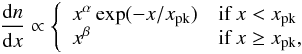 (24)where
dn/dx is the photon number density per dimensionless
energy interval. Because the number density of the photons of energy x is nph ~
xdn/dx ∝
xα+1 or
nph ∝
xβ+1 and the opacity
is proportional to nph according to Eq. (23), one finds that
(24)where
dn/dx is the photon number density per dimensionless
energy interval. Because the number density of the photons of energy x is nph ~
xdn/dx ∝
xα+1 or
nph ∝
xβ+1 and the opacity
is proportional to nph according to Eq. (23), one finds that
 for
for 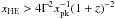 and
and  for
for 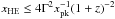 .
For a typical GRB with α ~ −1, the opacity remains relatively constant at
.
One also notes that the opacity increases for softer and decreases for harder bursts.
.
For a typical GRB with α ~ −1, the opacity remains relatively constant at
.
One also notes that the opacity increases for softer and decreases for harder bursts.
The number density nph is dominated by the prompt photons
while they are going through the shell of ejecta and can be estimated as  (25)which is obtained by
dividing the prompt GRB luminosity L by the volume covered by the photons per unit
time, 4πr2c,
and by the average energy of a photon, which we now assume to be the prompt peak energy
Epk.
(25)which is obtained by
dividing the prompt GRB luminosity L by the volume covered by the photons per unit
time, 4πr2c,
and by the average energy of a photon, which we now assume to be the prompt peak energy
Epk.
Using the expression for nph together with Eq. (23), one finds that τγγ ∝ r-1Γ-2 for high-energy photons for which the threshold energy is Epk. The prompt photons mainly overlap with the ejected shell during the coasting phase when Γ = Γ0 and r ∝ t. In this case, the optical depth evolves as τγγ ∝ r-1 ∝ t-1. After the deceleration time, r ∝ t1/4 and Γ ∝ r−3/2 in the ISM case, from which it follows that τγγ ∝ r2 ∝ t1/2. The probability for pair production is thus expected to decrease during the coasting phase but increase after RB if the prompt photons are still passing through the emission region. The rising opacity is due to the increasing angular spread of the emitted high-energy photons, which offsets the decrease due to the declining target photon density. Taking into account the beaming of the prompt radiation, the suppression of pair production is not exponential even at τγγ > 1. In this case there always exists an escape cone at sufficiently small angles, within which high-energy photons can escape. In a wind medium, where Γ ∝ r−1/2, τγγ ∝ r0 after the deceleration time, that is to say, the optical depth remains constant.
The above discussion on the pair production opacity applies to the high-energy photons for which the threshold energy of target photons is Epk, and the energy of the former is generally changing with time. However, if one assumes the canonical photon index α ~ −1, the photon number density nph ∝ xα+1 = x0 below the peak energy. In this case, the density of target photons below Epk is still given by Eq. (25) and the pair production opacities obtained above apply to any high-energy photon for which the threshold energy is below Epk.
Once the prompt photons have crossed the emission region, the synchrotron emission
provides the target photons for pair production with upscattered high-energy photons.
The number of synchrotron photons providing the pair production opacity is proportional
to the number of electrons emitting at xthr. The energy of these electrons
can be estimated from  (Eq. (16)), where xsyn is the
dimensionless synchrotron photon energy. This yields that the electron energy
corresponding to the threshold photon energy is γthr =
constant for a fixed xHE. In the slow cooling regime the
number of these electrons is Ne,thr ∝
r3(γthr/γmin)−s+1 ∝
r3Γs−1
(Eq. (15)). For example, in the ISM case
with s = 2
one gets an optical depth τγγ ∝
r2Γ ∝ t1/8 (Eqs. (10)
and (11)); i.e., the pair production
opacity is increasing in time, although very slowly.
(Eq. (16)), where xsyn is the
dimensionless synchrotron photon energy. This yields that the electron energy
corresponding to the threshold photon energy is γthr =
constant for a fixed xHE. In the slow cooling regime the
number of these electrons is Ne,thr ∝
r3(γthr/γmin)−s+1 ∝
r3Γs−1
(Eq. (15)). For example, in the ISM case
with s = 2
one gets an optical depth τγγ ∝
r2Γ ∝ t1/8 (Eqs. (10)
and (11)); i.e., the pair production
opacity is increasing in time, although very slowly.
3. Numerical treatment
3.1. Kinetic equations
The numerical code we use to simulate GRB afterglows is based on the code developed by Vurm & Poutanen (2009), which has successfully been applied to, say, modeling prompt GRB (Vurm et al. 2011) and black hole emission (Veledina et al. 2011, 2013). The code calculates the time-evolving particle distributions in an astrophysical plasma by solving the full relativistic kinetic equations for each particle species without any energy limitations. This means that the equations include both differential and integral terms, depending on the nature of each radiation process. If the energy losses of a particle are approximately continuous, differential terms are used to describe the process. An integral term is necessary if the particle loses a considerable fraction of its energy due to a single interaction. In this section, all quantities except for r and Γ are expressed in the fluid comoving frame and are left unprimed for ease of notation.
The equations for photons and electrons in the fluid comoving frame both have the same
general form (for a derivation, see, e.g., Blumenthal
& Gould 1970)  (26)where N ≡
N(x) (for photons) or N ≡
N(γ) (for electrons) is the particle
number density distribution in the shocked region per dimensionless photon or electron
energy interval. The subscripts syn, cs, pp and ad correspond to synchrotron emission and
absorption, Compton scattering, pair production and adiabatic cooling, respectively. Each
process produces a term on the right-hand side of the equation (for a detailed description
of the numerical treatment of the processes, see Vurm
& Poutanen 2009). The source term Qinj gives the
contribution of newly injected particles. The electron injection function is assumed to be
a pure power law (Eq. (13)) in most
examples presented in this paper. However, the injected electrons have a Maxwellian
distribution in some of the examples in Sect. 4.3.
The term N/tesc
accounts for the escape of particles from the emission region and N/texp
gives the dilution of the particle densities due to the expansion of the emission region,
tesc and texp being the
characteristic time scales for these processes. The adiabatic cooling and density dilution
terms are discussed in Sect. 3.3. The photon escape
time tesc is evaluated by solving the
plane-parallel radiative diffusion equation and is equal to
(26)where N ≡
N(x) (for photons) or N ≡
N(γ) (for electrons) is the particle
number density distribution in the shocked region per dimensionless photon or electron
energy interval. The subscripts syn, cs, pp and ad correspond to synchrotron emission and
absorption, Compton scattering, pair production and adiabatic cooling, respectively. Each
process produces a term on the right-hand side of the equation (for a detailed description
of the numerical treatment of the processes, see Vurm
& Poutanen 2009). The source term Qinj gives the
contribution of newly injected particles. The electron injection function is assumed to be
a pure power law (Eq. (13)) in most
examples presented in this paper. However, the injected electrons have a Maxwellian
distribution in some of the examples in Sect. 4.3.
The term N/tesc
accounts for the escape of particles from the emission region and N/texp
gives the dilution of the particle densities due to the expansion of the emission region,
tesc and texp being the
characteristic time scales for these processes. The adiabatic cooling and density dilution
terms are discussed in Sect. 3.3. The photon escape
time tesc is evaluated by solving the
plane-parallel radiative diffusion equation and is equal to
![Mathematical equation: \begin{equation} \tesc = \frac{3 \Delta R}{4 c}\left[1 + \frac{1-{\rm e}^{-\tstar}}{\sqrt{\epsilon}(1+{\rm e}^{-\tstar})}\right], \end{equation}](/articles/aa/full_html/2014/04/aa22520-13/aa22520-13-eq123.png) (27)where ΔR is the comoving radial
dimension of the emission region,
(27)where ΔR is the comoving radial
dimension of the emission region,  gives the effective optical depth and ϵ ≡ (αsyn +
αpp)/(αsyn
+ αpp + αcs) is
the probability for photon absorption, αsyn, αpp and
αcs being the extinction coefficients due
to synchrotron (syn) and pair production (pp) absorption and Compton scattering (cs).
gives the effective optical depth and ϵ ≡ (αsyn +
αpp)/(αsyn
+ αpp + αcs) is
the probability for photon absorption, αsyn, αpp and
αcs being the extinction coefficients due
to synchrotron (syn) and pair production (pp) absorption and Compton scattering (cs).
The code recalculates the radius r and bulk Lorentz factor Γ at each timestep according to Eqs. (2) and (7) and evaluates the observed time from Eq. (8). The other time-dependent quantities such as B, ṅel and γmin (Eqs. (12), (14) and (15)) can then be evaluated to obtain, for instance, the updated synchrotron emissivities.
The main difference between our code and the similar one described in PM09 is that we
include the second-order differential terms that correspond to electron heating and
diffusion due to synchrotron and Compton processes. The differential terms in the kinetic
equation for electrons take the form
![Mathematical equation: \begin{equation} \dot{N}(\gamma) = -\frac{\partial}{\partial\gamma}\left[\Ae(\gamma)N(\gamma)-\Be(\gamma)\frac{\partial N(\gamma)}{\partial\gamma}\right] \end{equation}](/articles/aa/full_html/2014/04/aa22520-13/aa22520-13-eq132.png) (28)for
all continuous processes, such as synchrotron processes, Compton scattering in the Thomson
regime and adiabatic cooling, and the coefficients Ae and
Be depend on the process of interest.
Synchrotron self-absorption also contributes a first- and second-order differential term
in the electron equation, where the coefficients Ae and
Be depend on the number density of photons
and the synchrotron emissivity of an electron.
(28)for
all continuous processes, such as synchrotron processes, Compton scattering in the Thomson
regime and adiabatic cooling, and the coefficients Ae and
Be depend on the process of interest.
Synchrotron self-absorption also contributes a first- and second-order differential term
in the electron equation, where the coefficients Ae and
Be depend on the number density of photons
and the synchrotron emissivity of an electron.
The kinetic equations are discretized and solved on finite grids of photon and electron/positron energies. Both the photon and electron energy grids consist of 200 points, with the photon grid ranging from x = 10-11 to x = 108 (E = 5 × 10⁻⁶eV to E = 50 TeV) and the electron grid ranging from p = 10-4 to p = 108.
Because of the high-energy boundary of the electron grid, the maximum energy of the
electrons is evaluated as  (29)The maximum Lorentz
factor
(29)The maximum Lorentz
factor  is obtained by comparing the acceleration time to the synchrotron cooling time. This is
the value used by our code as long as it does not exceed γ = 108, the
highest electron energy of the grid.
is obtained by comparing the acceleration time to the synchrotron cooling time. This is
the value used by our code as long as it does not exceed γ = 108, the
highest electron energy of the grid.
3.2. Size of the emission region
In the simulations presented here, we consider only the radiation from the forward shock. The current code applies a one-zone approximation by assuming that the particles behind the shock front are homogeneously distributed and that the magnetic field has a uniform value in the region of interest.
The emission region is the spherical shell between the forward shock and the contact
discontinuity that separates the shocked external medium and the shocked GRB ejecta. The
Lorentz factor of the forward shock is  (Blandford & McKee 1976), which means that the
contact discontinuity is moving away from the shock at a velocity c/3. This
leads us to define the radial extent of the shell as
(Blandford & McKee 1976), which means that the
contact discontinuity is moving away from the shock at a velocity c/3. This
leads us to define the radial extent of the shell as  (30)and the comoving volume
of the emission region becomes
(30)and the comoving volume
of the emission region becomes  (31)Here it is not
taken into account that the shell is most likely not spherical but a fraction of a narrow
jet. However, the luminosity per unit solid angle is the same in both of these cases
before the so-called jet break time, when the beaming angle of the radiation exceeds the
opening angle of the jet.
(31)Here it is not
taken into account that the shell is most likely not spherical but a fraction of a narrow
jet. However, the luminosity per unit solid angle is the same in both of these cases
before the so-called jet break time, when the beaming angle of the radiation exceeds the
opening angle of the jet.
3.3. Adiabatic cooling and density dilution
In addition to the radiation processes discussed in this paper, the code accounts for
adiabatic particle cooling due to the spreading emission region. In this section, all
quantities except for r are given in the fluid frame and are left unprimed.
The adiabatic cooling term for electrons is ![Mathematical equation: \begin{equation} \label{eq:ad} \nad \equiv \frac{\partial N(\gamma)}{\partial t} = -\frac{\partial}{\partial \gamma}\left[\gad N(\gamma)\right], \end{equation}](/articles/aa/full_html/2014/04/aa22520-13/aa22520-13-eq148.png) (32)where
(32)where
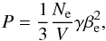
 is the cooling rate due to adiabatic expansion. The cooling rate is obtained from the
pressure P
and internal energy E of the electrons. For a monoenergetic population of
Ne electrons of energy γ in a volume
V,
is the cooling rate due to adiabatic expansion. The cooling rate is obtained from the
pressure P
and internal energy E of the electrons. For a monoenergetic population of
Ne electrons of energy γ in a volume
V,
 (33)where βe is the random
velocity of an electron in units of c, and
(33)where βe is the random
velocity of an electron in units of c, and
 (34)From the first
law of thermodynamics, dE = −PdV, one then obtains the cooling
rate
(34)From the first
law of thermodynamics, dE = −PdV, one then obtains the cooling
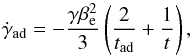
rate 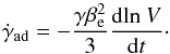 (35)Evaluating the
time derivative of the comoving volume (Eq. (31)), the cooling rate for a constant value of g (see Eqs. (3)−(6)) becomes
(35)Evaluating the
time derivative of the comoving volume (Eq. (31)), the cooling rate for a constant value of g (see Eqs. (3)−(6)) becomes
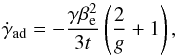 (36)where
t is the
comoving lifetime of the shock. Because the simulation extends from the coasting phase of
the relativistic shell to the deceleration phase, the value changes from g = 1 to g = 5/2
(constant density) or g = 3
/2 (wind) according to Eqs. (3) and (5) during the deceleration. This change is gradual in reality, but our
approximation of the Blandford-McKee solution has the side effect that the time derivative
of the volume and the cooling term of Eq. (36) are discontinuous at r =
RB. In order to avoid the
discontinuity, the cooling rate used in the simulations is
(36)where
t is the
comoving lifetime of the shock. Because the simulation extends from the coasting phase of
the relativistic shell to the deceleration phase, the value changes from g = 1 to g = 5/2
(constant density) or g = 3
/2 (wind) according to Eqs. (3) and (5) during the deceleration. This change is gradual in reality, but our
approximation of the Blandford-McKee solution has the side effect that the time derivative
of the volume and the cooling term of Eq. (36) are discontinuous at r =
RB. In order to avoid the
discontinuity, the cooling rate used in the simulations is
 (37)where
 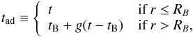 (38)tB being the
comoving time corresponding to the transition radius RB. This approach
guarantees that the adiabatic cooling term is continuous and that the solution is accurate
both at early and late times.
(38)tB being the
comoving time corresponding to the transition radius RB. This approach
guarantees that the adiabatic cooling term is continuous and that the solution is accurate
both at early and late times.
The term giving the dilution of the electron density (the last term on the right-hand
side of Eq. (26)) is obtained by
considering a constant number of particles with density n =
∫N(γ)dγ
in an expanding volume V:
 (39)This relation is
equivalent to
(39)This relation is
equivalent to 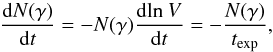 (40)where
 (41)and
tad is given by Eq. (38).
(41)and
tad is given by Eq. (38).
3.4. Test simulations
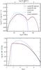 |
Fig. 1 Simulated afterglow spectrum in the observer frame (top panel) and the electron distribution in the fluid frame (bottom panel) at radius r = 3.4 × 1017 cm. The particle distributions have been obtained with four different combinations of radiative and adiabatic processes. Synchrotron emission/absorption, Compton scattering, pair production/annihilation and adiabatic energy losses are indicated in the figure by the abbreviations syn, IC, pp and ad, respectively. In the simulation where only synchrotron processes are included, self-absorption heating of the electrons is not accounted for. The analytic synchrotron solution by Sari et al. (1998) is also shown in the figures. The simulation parameters are E0 = 1053erg, n0 = 1 cm-3, ϵe = 0.1, ϵB = 10-3, Γ0 = 400 and s = 2.3. The high-energy cutoff of the electron distribution has a constant value γmax = 4 × 10⁷, and the GRB is located at a redshift z = 1. In the bottom panel, N(γ) ≡ dn/dγ is the number density of electrons per dimensionless energy interval. The distribution function has been multiplied by σTΔR′ to find the Thomson optical depth and by γs in order to visualize which electrons are cooling: a flat segment in the distribution means that the slope is the same as that of the injection function, demonstrating that the electrons are uncooled. The figure may be compared with Figs. 4 and 5 of PM09. |
In order to test the validity of our code, we have compared our simulation results with those obtained by PM09 who have developed a similar numerical code. The photon spectra and electron distributions at r = 3.4 × 1017 cm (Fig. 1) calculated by our code should be compared with Figs. 4 and 5 of PM09, which present the particle distributions obtained with the same set of parameters. In these simulations, a constant value of the maximum electron energy, γmax = 4 × 10⁷, is assumed. Our Fig. 1 shows the results of several simulations with different combinations of radiation processes. All the photon spectra in this section and the rest of the paper are presented in the observer frame, with energies boosted by a factor of 2Γ/(1 + z) from the flow frame.
The two codes produce electron distributions with very similar shapes: the cooled electrons populate the high-energy end of the distribution going as N(γ) ∝ γ−s−1, with the slope of the distribution gradually approaching the slope of the injection function at lower energies. The electrons below γmin ~ 600 have a nearly flat N(γ) distribution in PM09, whereas we obtain a much steeper decline of the electron density. To study whether this difference could be due to the inclusion of synchrotron self-absorption heating, we turned off this process for a test simulation, but this had no visible impact on the electron distribution. Because the shell is in the deceleration phase and γmin is decreasing, such a steep cutoff may appear if γmin declines faster than the electrons are cooled adiabatically. However, the electrons below γmin do not carry a large fraction of the total electron energy and have no observable impact on the afterglow emission.
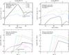 |
Fig. 2 Left panels: time-evolving observer frame photon spectrum without absorption on extragalactic background light (top panel) and electron distribution (bottom panel) from the forward shock together with an additional photon injection term that roughly represents prompt GRB emission. The electron distributions are plotted as a function of the dimensionless electron momentum p (Eq. (1)) instead of γ (note that p → γ for γ ≫ 1). The number of electrons per unit dimensionless momentum is N(p) ≡ dn/dp. The parameters of the forward shock emission are E0 = 1.4 × 1055 erg, n0 = 3 × 10⁻² cm-3, ϵe = 0.2, ϵB = 10-6, Γ0 = 800 and s = 2.4. The injected photons are distributed according to a Band function, with the parameters α = −0.61, β = −3.8 and Epk = 730 keV (as defined in Eq. (24)). The Band function cuts off at E = 1 GeV and the injection lasts for t = 22 s, after which the photon luminosity decreases exponentially with time. The GRB takes place at z = 1.8. The black long-dashed lines show the photon and electron distributions at t = 0.1 s without pair production, and the solid magenta line in the bottom left panel represents the positron distribution at t = 0.1 s. Right panels: the evolution of the observer frame photon spectrum (top panel) and electron distribution (bottom panel) without photon injection. The forward shock parameters are same as in the simulation presented in the left panels. |
The normalization of our electron distribution is lower by about half an order of magnitude than that obtained by PM09, but the origin of this difference is unclear so far. In our radiation spectrum, the spectral slopes and the positions of the peak and break frequencies appear identical to those in PM09, but the normalization of the flux is again slightly different. It is notable that the relative magnitudes of the synchrotron and inverse Compton components are clearly different in the two simulations. A possible cause for this discrepancy is the slight difference in the geometries assumed in the simulations.
The electron distribution resulting from synchrotron cooling without adiabatic cooling or self-absorption heating is also presented in Fig. 1, showing that especially the low-energy electrons are strongly affected by adiabatic cooling. The distribution around the cooling break is highly curved without this process, and there is a clear cutoff below the injection energy γmin since the electrons no longer have a way to cool to lower energies.
The radiation spectrum from this simulation is also presented in Fig. 1. The curved part of the electron distribution produces a corresponding curved segment in the radiation spectrum. The low-energy end of the spectrum, which basically consists of radiation from monoenergetic electrons at γmin, has the same shape in all cases. All in all, adiabatic cooling has a clear observable effect on the emergent spectrum but the contribution of synchrotron self-absorption heating seems negligible.
The analytic synchrotron solution by Sari et al. (1998) is included in Fig. 1 for comparison with the numerical solution. It is clear that a spectrum consisting of pure power-law segments with sharp breaks deviates from the actual curved synchrotron radiation component, and fitting the simple analytic model to observed afterglow spectra may lead to an inaccurate determination of the forward shock parameters.
4. Examples
4.1. High-energy emission due to Compton scattering of MeV photons
As an example of an important application of the code, we present the results of two simulations where the injected electrons interact with an external source of photons distributed according to a Band function (Eq. (24)), which represents a typical prompt GRB spectrum. Some of the GRB photons are scattered to higher energies by the shock-accelerated electrons, producing an additional spectral component extending up to TeV energies in the observer frame. The high-energy end of the spectrum can then be further modified as some of the high-energy photons produce electron-positron pairs with the MeV photons. The ≳TeV component may be observable in the case of a low-redshift GRB; otherwise the very high-energy gamma-rays are absorbed by the extragalactic background light. The simulations presented here demonstrate that our code can be applied to study whether the >100 MeV GRB emission is due to Compton scattering of the prompt photons at the external shocks. However, further modifications of the code are needed to improve especially the treatment of the early high-energy emission.
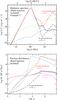 |
Fig. 3 Time-evolving observer frame photon spectrum without absorption on extragalactic background light (top panel) and electron distribution (bottom panel) from the forward shock with the same photon injection term as in Fig. 2. The other simulation parameters are E0 = 1.4 × 1055erg, n0 = 3 cm-3, ϵe = 0.8, ϵB = 10-8, Γ0 = 450 and s = 2.4. The redshift is z = 1.8. The black and red long-dashed lines show the photon and electrons distributions at t = 0.1 s and t = 10 s without pair production, and the positron distribution at t = 0.1 s is presented by a solid magenta line in the bottom panel. |
The current version of the code calculates the emission from the forward shock only, although the reverse shock emission can be significant in the case of a long burst. In addition, electron-positron pair production in the external medium due to the interaction with the prompt gamma-rays is likely to affect the afterglow emission (Beloborodov 2005a). This effect is not accounted for in the code at the moment. However, both the reverse shock emission and the pair loading of the external medium are expected to shape the afterglow at relatively early times, and thus the late-time afterglow emission is likely to be fairly consistent with the results of the forward shock simulation.
Figure 2 shows the simulated time-evolving forward shock spectrum and the corresponding electron distribution both with and without an additional Band injection term, and Fig. 3 presents the results of a simulation with the same Band injection function but different external shock parameters. The positron distribution at t = 0.1 s is also presented in the cases where pair production is important, meaning in the simulations with a photon injection term. At the moment, the positron distribution has a lower numerical accuracy than that of the electrons.
The simulation parameters have been chosen to reproduce the Swift/XRT
afterglow light curve of GRB 090902B, which was a bright burst with a long-lasting
high-energy component (Abdo et al. 2009). The Band
function used in the simulations is kept constant in time for simplicity and corresponds
to the time-integrated spectral fit presented in Table 1 of Abdo et al. (2009). The Band photon density nph in the
observer frame is evaluated from Eq. (25),
where the luminosity is obtained from dividing the isotropic equivalent energy of the
prompt GRB, Eiso =
3.6 × 1054 erg, by the burst duration, t = 22 s. The number of
injected photons per unit time and area is then ~cnph in the observer
frame, and the injection rate per unit volume in the fluid frame is
 (42)where the shell thickness
ΔR′ is defined in Eq. (30). We do not inject the additional power-law
component that is observed in the prompt emission below ~50 keV and above 100 MeV.
(42)where the shell thickness
ΔR′ is defined in Eq. (30). We do not inject the additional power-law
component that is observed in the prompt emission below ~50 keV and above 100 MeV.
The allowed forward shock parameter space based on the late-time afterglow data has been calculated by Kumar & Barniol Duran (2010), who claim that the >100 MeV emission can be explained as pure synchrotron radiation. The simulations presented in this section correspond to two points in the allowed n − ϵB space given in Figure 3 of their paper, with E0 and ϵe being evaluated from their Eqs. (12) and (13). Our Fig. 2 shows the results in the case of a lower density and a higher magnetic energy fraction than in Fig. 3. We assume that the ejecta begin to decelerate at the end of the prompt burst. This assumption is used to evaluate the initial bulk Lorentz factor of the emitting shell, Γ0. The extragalactic background light absorption of the ≳TeV photons is not accounted for in the example presented here, and these photons would in fact be unobservable from the redshift of GRB 090902B, z = 1.8. However, a very high-energy component could be observed in the case of a low-redshift burst with similar parameters.
The left-hand panels in Fig. 2 show that the Band emission at energies E ≲ 1 GeV dominates over the underlying forward shock synchrotron radiation at t = 0.1 s, while a double-peaked inverse Compton component appears at higher energies. The break at ~100 GeV is due to pair production with the peak Band photons, which are located at the threshold energy for pair production with the photons at ~100 GeV according to Eq. (22). For target photons with a Band distribution, the optical depth peaks at ~10xthr, where the lowest point between the two VHE spectral peaks is located. The maximum optical depth can be approximated using Eqs. (23) and (25) to obtain τγγ ~ a few. The importance of pair production can be confirmed by looking at the electron and positron distributions, which are nearly identical below γmin ~ 105. The VHE peak in the radiation spectrum is due to the scattering of Band photons against the peak electrons with γpk = γmin. According to Eq. (20), the peak energy is E ~ 30 TeV, which agrees with the figure.
The right-hand panels, showing the results of the simulation without the Band injection term, confirm that the synchrotron spectral component at t = 0.1 s is clearly below the Band emission, and the contribution from the Compton scattered synchrotron photons is also negligible. In the simulation with the additional photon injection term, a low-energy tail forms in the electron distribution. This is mainly caused by pair production with a contribution from scatterings in the K-N regime, which can take a large fraction of the energy of an electron in one scattering.
At t = 10 s, close to the deceleration time, the IC component has only one peak left in both simulations. The optical depth for pair production is expected to decrease until the deceleration time according to τγγ ∝ t-1 and thus should drop by a factor of 100 between t = 0.1 s (where τγγ ~ 2) and t = 10 s, which is in agreement with the simulation results. In the left panels, the prompt emission dominates as the source of seed photons for inverse Compton, as the resulting high-energy emission is ~2 orders of magnitude more luminous than with synchrotron self-Compton (SSC) emission alone. The high-energy part of the synchrotron bump has become visible at t = 10 s and dominates the emission at E ~ 100 MeV−10 GeV. The inverse Compton peak is still located at E ~ 30 TeV, and it seems that the prediction for the location of the peak is very robust during the prompt emission due to the hard spectrum of the soft target photons. In the slow cooling regime and in the absence of significant pair opacity, the spectral slope below the ~30 TeV peak mimics the low-energy slope of the prompt spectrum. Because the peak energy is proportional to Γγmin and γmin ∝ ϵeΓ, a measurement of the peak energy would provide us with the combination ϵeΓ2.
After the end of the photon injection, the spectrum quickly becomes identical to the pure forward shock emission, as can be seen by comparing the spectra at t = 103 s and t = 105 s in the left and right panels. The electrons are unable to cool by emitting synchrotron radiation because such a small fraction of the shock energy is given to the magnetic field. The SSC cooling of the electrons on synchrotron radiation is not effective either, which can be seen from the electrons being distributed as N(γ) ∝ γ−s between γmin and γmax. The synchrotron spectral component produced by these electrons now corresponds to a slow cooling spectrum as described by Sari et al. (1998).
The simulation results presented in Fig. 3 correspond to a higher density and smaller magnetic energy density than those in Fig. 2. The VHE spectrum at t = 0.1 s is similar to the one in Fig. 2. In this case, the spectrum at t = 10 s is also shaped by the inclusion of pair production, which leads to an increased energy content in electrons at γ<γmin and correspondingly more energy in the upscattered photons between ~3 GeV and ~1 TeV. After the prompt emission is gone, the SSC component is very prominent compared to the synchrotron bump because of the high value of ϵe/ϵB used in the simulation. Even though a large fraction of the shock-generated energy, ϵe = 0.8, is given to the electrons now, it is still valid to assume an adiabatic evolution of the shock because the radiative cooling is inefficient.
It is notable that a power-law component similar to the one observed during the prompt
phase of GRB 090902B (Abdo et al. 2009) is not seen
in our simulations. According to the simple model presented here, the early power-law
component cannot be of external origin. The low-energy part of the component might be
detectable above the Band emission in the case of a low γmin (Eq. (15)). Because we assume that the deceleration
time is approximately equal to the duration of the prompt GRB, we can use Eqs. (4) and (9) in our paper, together with Eqs. (12) and (13) in Kumar & Barniol Duran (2010) to find that
 ; i.e.,
γmin depends very weakly on
n and
ϵB. From the allowed
n −
ϵB space presented in
Fig. 3 of Kumar & Barniol Duran (2010), one
finds that γmin cannot be much lower than
~105.
; i.e.,
γmin depends very weakly on
n and
ϵB. From the allowed
n −
ϵB space presented in
Fig. 3 of Kumar & Barniol Duran (2010), one
finds that γmin cannot be much lower than
~105.
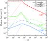 |
Fig. 4 Observer frame light curves in the Swift/XRT band (0.3−10 keV, red curves at the top of the figure), the Fermi/LAT band (0.1−300 GeV, green curves in the middle), and a very high energy (VHE) 0.1−100 TeV band (blue curves at the bottom). The light curves correspond to the simulations presented in Figs. 2 and 3. |
Figure 4 shows the light curves corresponding to the simulations presented in Figs. 2 and 3 (Band injection is included in Examples 1 and 3, but not in Example 2) in three different energy bands: the XRT and LAT bands and a very high-energy (VHE) band ranging from 0.1 TeV to 100 TeV, where the only contribution is from the inverse Compton emission due to the upscattering of either synchrotron or external photons. Because the Band function is kept constant in time, the flux in both the XRT and LAT bands is also constant in the beginning of the simulations with the photon injection term. The inverse Compton flux in the VHE band rises at early times as the energy of the shocked electrons increases and the suppression of the flux due to pair production becomes less important.
The LAT light curves are dominated by synchrotron emission between t ~ 10 s and 103 s. At 103 s the synchrotron component falls below the LAT band and there is a break in the light curves, followed by a more slowly decaying SSC emission. The X-ray emission from the forward shock is buried under the prompt emission and emerges only after the latter has ended. In the TeV band the emission is dominated by the upscattered prompt photons as long as they are available, resulting in substantially higher luminosity at early times than would be obtained by SSC alone.
The simulated XRT band light curves are consistent with the observed XRT data of GRB 090902B (Pandey et al. 2010) as intended, but the observed LAT light curve (Abdo et al. 2009) is not reproduced in the current simulations. This is simply because we assume a lower value of γmax (Eq. (29)) than Kumar & Barniol Duran (2010), who claim that the high-energy emission consists of synchrotron photons. The maximum photon energy produced by the synchrotron process is ~2Γ × 50 MeV/(1 + z) in the observer frame (Guilbert et al. 1983), determined from the balance between the cooling and acceleration times for electrons radiating in the background magnetic field B′ (for synchrotron losses taking place in a magnetic field generated by the Weibel instability, see Sironi et al. 2013). The most energetic photon observed from GRB 090902B, with E = 33 GeV in the observer frame, requires a bulk Lorentz factor Γ ~ 900 at t = 82 s to be consistent with the synchrotron model. The Lorentz factor at this time can be estimated from Eq. (11). For E0 ~ 1055erg and n0 = 10-3 cm-3, the lowest possible external density according to Kumar & Barniol Duran (2010), we find that Γ ~ 400 at t = 82 s, not supporting a synchrotron origin for this photon.
The examples in this section show that a luminous ≳TeV component can arise due to inverse Compton scattering in the forward shock, although this radiation is observable only in low-redshift cases. The Cherenkov telescope MAGIC is the most likely candidate to catch the upscattered prompt radiation in the VHE range due to its fast slewing capability, but MAGIC has so far been unable to detect any emission from GRBs (Albert et al. 2007; Aleksić et al. 2010, 2014). However, the lack of detections does not rule out the existence of a ~10 TeV spectral component because of the high redshifts of the observed bursts.
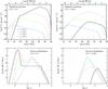 |
Fig. 5 Left panels: time-evolving observer frame photon spectrum (top panel) and electron distribution (bottom panel) resulting from synchrotron emission and absorption together with adiabatic cooling at the forward shock in a wind-type medium. The simulation parameters are E0 = 1054erg, Aw,35 ≡ Aw/(1035 cm-1) = 3, ϵe = 0.1, ϵB = 0.1, Γ0 = 500 and s = 2.5. The redshift is z = 1. Right panels: observed photon spectra (top panel) and electron distributions (bottom panel) in the case of a constant-density medium with a typical density n0 = 1 cm-3. The other simulation parameters are the same as in the simulation presented in the left panels. |
If the external density were higher than in our examples, such as in the case of a wind-type medium, the inverse Compton flux would also increase and possibly be able to reproduce the magnitude of the GeV photon flux in the LAT band. This idea is supported by the recent simulations of Beloborodov et al. (2013), who show that the GeV emission of GRB 080916C is consistent with inverse Compton scattering of the prompt emission. The work of Beloborodov et al. (2013) is mainly concerned with the early stage of the outflow and does not include SSC emission, which is important once the prompt radiation is gone.
Our current model cannot explain the extended duration of the observed LAT emission from GRB 090902B, which is however reproduced by Beloborodov et al. (2013). The delay of the arrival times of the high-energy photons compared to the MeV emission may result from the different propagation angle of the Compton scattered prompt photons compared to that of the unscattered photons, which is not accounted for in the code at the moment. It must be noted that a full treatment of the afterglow requires a more complete model of the prompt emission, the inclusion of the reverse shock emission and the effect of the pair loading of the external medium.
4.2. Constant-density ISM vs. wind medium
The density structure of the ambient medium has an impact on the evolution of the bulk Lorentz factor Γ, the injection rate of the electrons and the strength of the shock-compressed magnetic field. In a wind-type medium with n(r) = Awr-2 all the synchrotron-emitting electrons are likely to be fast-cooling at early times because of the high magnetic field, provided that the magnetization parameter ϵB is not too low. Synchrotron cooling is counteracted by self-absorption at the low-energy end of the distribution. As long as the synchrotron cooling time of the electrons is shorter than the lifetime of the flow for all electron energies, the low-energy electrons are able to thermalize due to self-absorption.
The difference between the pure synchrotron emission from the forward shock in a wind-type and a constant-density medium is illustrated in Fig. 5, which shows the simulated photon and electron distributions for a typical set of parameters. Compton scattering and pair production are left out of this simulation in order to study the effect of synchrotron self-absorption heating on the particle distributions. Again, we assume that the distribution of the shock-accelerated electrons is a pure power law.
The deceleration radius (Eqs. (4) and (6)) is reached earlier in a wind medium than a constant-density ISM. In the simulations presented in Fig. 5, Rdec = 7.1 × 1014 cm in the wind case and Rdec = 8.6 × 1016 cm in the ISM case. Because most of the blast energy is dissipated at this radius, the peak luminosity is higher in the wind case because the same amount of energy is emitted in a shorter time compared to the ISM environment.
At the observed time t =
0.1 s, the ambient particle density in the wind case is n = 1.1 ×
106 cm-3, explaining the large difference between
the number of shocked electrons in the two simulations. At this moment, all the electrons
are fast-cooling in both simulations due to the large fraction of energy given to the
magnetic field. However, the magnetic field in the wind case is much higher because of the
high density, even though the shock has already entered the deceleration phase before
t = 0.1 s.
The electrons have now been able to cool below γmin and form a clear Maxwellian
component centered at γ ~
3. The Maxwellian electrons have had plenty of time to thermalize
because their synchrotron cooling time in the fluid comoving frame,
 (Eqs. (12) and (19)) is clearly shorter than the comoving lifetime of the flow,
t′ =
40 s. The electrons at higher energies are distributed according to
N(γ) ∝
γ-2 below γmin and
N(γ) ∝
γ−s−1 between
γmin and γmax, as
expected. It is notable that the electrons would be able to cool to much lower energies in
a simulation without the self-absorption heating term. Thus, the inclusion of this term is
necessary for the modeling of a wind-type medium with a high magnetic compactness. The
thermalized electrons, however, only produce a very small bump in the corresponding
synchrotron spectrum.
(Eqs. (12) and (19)) is clearly shorter than the comoving lifetime of the flow,
t′ =
40 s. The electrons at higher energies are distributed according to
N(γ) ∝
γ-2 below γmin and
N(γ) ∝
γ−s−1 between
γmin and γmax, as
expected. It is notable that the electrons would be able to cool to much lower energies in
a simulation without the self-absorption heating term. Thus, the inclusion of this term is
necessary for the modeling of a wind-type medium with a high magnetic compactness. The
thermalized electrons, however, only produce a very small bump in the corresponding
synchrotron spectrum.
At t = 10 s, the Maxwellian component in the electron distribution in a wind medium is already smaller because of the decreasing magnetic field. The bump gradually disappears, and the slope of the electron distribution at t = 105 s between γc ~ 600 and γmin ~ 3 × 10³ is becoming slightly shallower because these electrons are no longer able to cool. At this moment, the electron and photon distributions in the ISM case look very similar to those in the wind case.
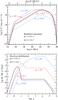 |
Fig. 6 Comparison of the radiation spectrum (top panel) and electron distribution (bottom panel) at t = 0.1 s from Fig. 5 (black solid line) to four cases where the value of one parameter is changed at a time. In two simulations, the wind density is decreased by a factor of 10 (red dashed line) and 100 (blue dashed line) from the fiducial value. In the other two cases, the magnetic energy fraction is decreased by a factor of 102 (red dash-dot line) and 104 (blue dash-dot line). |
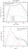 |
Fig. 7 Time evolution of the observer frame photon spectrum (top panel) and electron distribution (bottom panel) in a wind medium when all the relevant radiative processes (synchrotron, Compton and pair production) are accounted for in the simulation. The positron distribution at t = 0.1 s is also shown as a solid magenta line in the bottom panel. The simulation parameters are the same as in Fig. 5. |
The simulations presented here show that the synchrotron self-absorption heating of electrons can produce a prominent Maxwellian component in the electron distribution for certain parameter sets. Figure 6 shows how the size of the Maxwellian bump at t = 0.1 s decreases if the parameters ϵB and Aw are changed from the fiducial values used to obtain Fig. 5 and how this affects the corresponding synchrotron spectrum. When the magnetic energy fraction ϵB is decreased, the synchrotron cooling time is longer and the electrons are unable to cool to very low energies or thermalize efficiently.
The magnetic field and the size of the thermalized bump also decrease if the density of the wind goes down: when the coefficient Aw,35 ≡ Aw/(1035 cm-1) is decreased from Aw,35 = 3 by a factor of 100, the low-energy bump in both the electron and photon distributions has nearly disappeared. It should be noted that the bulk Lorentz factor Γ is lower in the simulation with Aw,35 = 3 compared to the two cases with different Aw,35, because the shock is already in its deceleration phase at t = 0.1 s with Γ ~ 300 in the case with the highest density. As a result, the shock radius is slightly smaller in the case of a decreasing Γ, but only by a factor of ~ a few.
In general, the magnetic field (see Eq. (12)) decreases at radii r<Rdec
(Eq. (6)) due to the radial dependence of
the wind density: 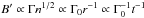 ,
so a larger Γ0
indicates a lower magnetic field B′ at a given observer time
t as long
as the blast is its coasting phase. The synchrotron cooling time of the electrons thus
becomes longer, working against the formation of a Maxwellian component.
,
so a larger Γ0
indicates a lower magnetic field B′ at a given observer time
t as long
as the blast is its coasting phase. The synchrotron cooling time of the electrons thus
becomes longer, working against the formation of a Maxwellian component.
The deceleration radius Rdec depends on the parameters
E0,Aw
and Γ0 but the
hydrodynamic evolution at r > Rdec
is only affected by E0 and Aw according to
Eqs. (10) and (11). The magnetic field then depends on these
parameters and time as 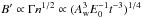 (naturally, B′ also depends on ϵB). Together with the
width of the emission region, ΔR′ ∝ Γt (Eq. (30)), the magnetic field determines the
magnetic compactness lB ≡
ΔR′UBσT/(mec2), where
UB =
(B′)2/(8π) is the magnetic energy density. An electron with
a random Lorentz factor γ is able to cool due to synchrotron emission if the
ratio t/tcool ~
γlB (see Eq. (19)) is large. Because
(naturally, B′ also depends on ϵB). Together with the
width of the emission region, ΔR′ ∝ Γt (Eq. (30)), the magnetic field determines the
magnetic compactness lB ≡
ΔR′UBσT/(mec2), where
UB =
(B′)2/(8π) is the magnetic energy density. An electron with
a random Lorentz factor γ is able to cool due to synchrotron emission if the
ratio t/tcool ~
γlB (see Eq. (19)) is large. Because
 , one can
obtain lower values of t/tcool
at a given time by increasing E0 or decreasing Aw, which may
prevent the thermalization at low energies.
, one can
obtain lower values of t/tcool
at a given time by increasing E0 or decreasing Aw, which may
prevent the thermalization at low energies.
In reality, pair production has a significant effect on the external shock emission as long as the wind density is high. Figure 7 presents the time-evolving radiation spectrum and electron distribution from a simulation where synchrotron, Compton and pair production processes are all accounted for. At t = 0.1 s, the interplay of these processes results in a complex shape of the electron and positron distributions for γ< 100. Numerous leptons appear at these energies because of pair production, and are able to thermalize at low energies due to the high magnetic compactness. However, the Maxwellian leptons are now non-relativistic and do not result in an observable signature in the corresponding photon spectrum. The spectrum at t = 0.1 s is clearly different from the pure synchrotron case in Fig. 5. In Fig. 7, the electrons at γ< 100 produce a distinct spectral segment between ~100 eV and 100 keV, and pair production shapes the synchrotron and Compton components at high energies. The pair production opacity decreases at later times and the spectrum becomes similar to the pure synchrotron case, with the obvious exception that it extends to higher energies because of Compton scattering.
4.3. Emission from a Maxwellian distribution of injected electrons
Because a Maxwellian component can contain as much as ~90% of the energy of the shocked electrons (Spitkovsky 2008), we have also simulated the forward shock emission
resulting from a Maxwellian electron injection function. The relativistic Maxwellian has
the general form ![Mathematical equation: \begin{equation} N(\gamma) \propto \gamma\sqrt{\gamma^2-1}\exp{\left[-\frac{\gamma}{kT'/\left(\mel c^2\right)}\right]}, \end{equation}](/articles/aa/full_html/2014/04/aa22520-13/aa22520-13-eq292.png) (43)where T′ is the
temperature of the electrons. The temperature can be determined from
(43)where T′ is the
temperature of the electrons. The temperature can be determined from  (44)where
ϵeΓmpc2
is the average energy transferred to a shocked electron.
(44)where
ϵeΓmpc2
is the average energy transferred to a shocked electron.
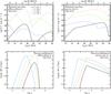 |
Fig. 8 Left panels: time evolution of the observer frame photon spectrum (top panel) and electron distribution (bottom panel) resulting from relativistic Maxwellian electron injection in a constant-density ISM. The radiation processes are synchrotron emission/absorption, Compton scattering and pair production/annihilation. The simulation parameters are E0 = 1052erg, n0 = 1 cm-3, ϵe = 10-2, ϵB = 10-4 and Γ0 = 200, and the redshift is z = 1. The Maxwellian injection function has the temperature T′ ~ ϵeΓmpc2/k. Right panels: evolving particle distributions in the case of a power-law electron injection with s = 2.5. The other parameters are the same as in the simulation with Maxwellian injection. |
A comparison between the simulated photon and electron distributions resulting from Maxwellian and power-law electron injection in a constant-density ISM is presented in Fig. 8. Synchrotron, Compton and pair production processes are all included in these examples. The main difference between the two cases is the width of the synchrotron component, which extends to higher energies when a large fraction of the electron energy is in the power-law electrons above the peak Lorentz factor.
In both simulations, the low-energy part of the synchrotron spectrum at t = 0.1 s and t = 10 s consists of the tail emission from the peak electrons, having the spectral shape νFν ∝ ν4/3. The synchrotron spectral component is naturally broader in the case of power-law electron injection, since the radiating electrons in the case of Maxwellian injection are nearly monoenergetic. The ~10 TeV inverse Compton peak is due to the scattering events by the electrons near the K-N limit. At t = 105 s, a second Compton scattering order appears as the first scattering order moves to ~100 eV. At all times, a Maxwellian electron injection results in a spectrum consisting of distinctly separate components, which is very different from the case of power-law electron injection.
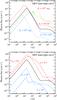 |
Fig. 9 Observer frame light curves in the Swift/XRT band (0.3−10 keV) resulting from different parameter sets. The black solid line in both panels shows the fiducial light curve resulting from Maxwellian electron injection obtained with the same parameters as the spectra in Fig. 8. The green dash-dot-dot-dot line in the top panel represents the emission due to a power-law electron injection function. The other curves represent simulations with a Maxwellian injection term where one parameter at a time is varied from the fiducial value. In the top panel, the dotted (dashed) lines show the light curves when the blast energy E0 (external density n0) is increased/decreased by a factor of 100 (10). In the bottom panel, the long-dashed (dash-dot) lines correspond to the emission when the electron energy fraction ϵe (magnetic energy fraction ϵB) is increased/decreased by a factor of 10 (100). |
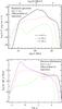 |
Fig. 10 Evolving photon (top panel) and electron (bottom panel) distributions from a simulation with Maxwellian electron injection in a wind-type medium. The magenta line in the bottom panel shows the positron distribution at t = 0.1 s. The simulation parameters are the same as in Fig. 8, except for ϵe = 0.1 and Aw,35 = 3. |
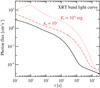 |
Fig. 11 Observer frame Swift/XRT band light curves in the case of Maxwellian electron injection in a wind medium. The solid line is the fiducial light curve corresponding to Fig. 10. The dotted (dash-dot) curve is obtained by increasing E0 (ϵB) by a factor of 100 from the fiducial value. |
Figure 9 shows the light curves in the Swift/XRT band resulting from both the simulations in Fig. 8 compared to several cases where one parameter at a time is changed. It is notable that a flattening or a slight rebrightening appears in all the cases with a Maxwellian electron injection. The flat segment is produced when the synchrotron component moves out of the observed energy range and is gradually replaced by the inverse Compton emission, similarly as described by Petropoulou et al. (2011), who simulated the external shock emission from power-law electrons with a narrow energy distribution. A similar effect is also seen in the simulations of Stern & Poutanen (2004). They considered prompt GRB emission due to a narrow electron distribution that has developed due to the balance between heating and synchrotron/SSC cooling. In this case, a flat section in the BATSE band light curve develops when the first Compton scattering order moves out of the observed band and is replaced by the second scattering order. A spectrum due to power-law electrons does not contain such dramatic changes of the spectral slope, and consequently there is no shallow decay segment in the light curve.
In all the cases shown in Fig. 9, the flux during
the flattening or rebrightening is very low. The flux is higher when E0,
n0, ϵe or
ϵB is increased, but
higher values of E0,ϵe
and ϵB also lead to a
delayed start of the flat segment. One can estimate that the flattening begins when the
synchrotron frequency of the peak Maxwellian electrons decreases below the observed
waveband. The peak electrons have γ ~
Γϵemp/me
(Eq. (44)) and the characteristic
synchrotron energy of the emitted photons is 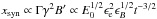 (see
Eqs. (16), (11) and (12)).
Increased values of E0,ϵe
and ϵB thus correspond to a
higher synchrotron energy at a given time t, delaying the moment when the synchrotron bump
crosses the observing window. However, a higher external density n0 does not
significantly delay the appearance of the shallow decay.
(see
Eqs. (16), (11) and (12)).
Increased values of E0,ϵe
and ϵB thus correspond to a
higher synchrotron energy at a given time t, delaying the moment when the synchrotron bump
crosses the observing window. However, a higher external density n0 does not
significantly delay the appearance of the shallow decay.
A more luminous shallow decay phase may occur in a wind-type medium. The particle distributions resulting from a Maxwellian electron injection function in a wind-type medium are presented in Fig. 10. Similarly as in the case of power-law injection in a wind environment (Fig. 7), pair production shapes the electron distribution for γ< 103 at t = 0.1 s, where it is practically identical to the positron distribution. However, we are now interested in the spectral evolution at later times when the shallow decay may appear as the observing window becomes dominated by inverse Compton photons. Figure 11 shows that the flux during the shallow decay can be high enough to be detected in the wind case. In the simulation presented here, the flux decay is steeper during this phase than in the ISM case, but still consistent with many of the observed XRT afterglows. The flux increases with higher values of, say, E0 and ϵB, but simultaneously the start of the shallow decay is delayed, as described above.
The simulations with different parameter sets show that a flattening in the X-ray light curve is likely to take place if the electron injection function is Maxwellian. In the ISM case, the flux during the simulated flattening appears to be much lower than a typical shallow decay flux observed by XRT. A wind environment, on the other hand, can lead to a detectable photon flux during the shallow decay.
5. Summary and conclusions
In this paper, we have studied the modeling of GRB forward shock emission for the first time with a code that treats all the radiation processes self-consistently. The main advantages of our code are the inclusion of synchrotron self-absorption heating and Compton scattering as mechanisms for electron thermalization, and the exact treatment of Compton scattering and pair production. We have shown that our results are in very good agreement with both analytic estimations and numerical simulations that have been presented in the literature. Inclusion of an accurate calculation of radiative transport, a multi-zone treatment of the emitting region, and the emission from the reverse shock will be the topics of future research.
We presented the results of test simulations where external MeV photons, distributed similarly to prompt GRB emission, interact with the shock-accelerated electrons and are Compton scattered to TeV energies. Such VHE emission is likely to dominate the synchrotron self-Compton emission at times up to t ≳ 10 s in GRBs with similar parameter sets and might be an interesting target for observations of low-redshift bursts with future instruments such as the Cherenkov Telescope Array (Inoue et al. 2013). We also showed that the inverse Compton flux is not always quenched by electron-positron pair production, owing to the decrease in the pair production opacity before the deceleration time. A very prominent inverse Compton peak appears during the prompt emission, the location of which is determined by the maximum energy given to the photons by the peak electrons.
Even though the test simulations show that the inverse Compton scattering of photons distributed according to a Band function is likely to produce a high-energy spectral component, the current model does not explain the typical long duration of the observed LAT emission in the case of GRB 090902B. A possible explanation for the LAT data is that the unscattered prompt photons are traveling within a smaller solid angle than the scattered photons, and the arrival time of the upscattered radiation is delayed as a result (Beloborodov 2005b; Beloborodov et al. 2013). This effect is not accounted for in the current version of the code. However, the large-angle effect cannot explain the LAT emission if it lasts much longer than the prompt GRB.
As another example, we compared the synchrotron emission in a wind-type and a constant-density ISM medium for a set of typical parameters and studied the effect of different simulation parameters on the thermalization of low-energy electrons. As long as the synchrotron cooling time is shorter than the lifetime of the flow, the low-energy end of a power-law electron distribution is strongly thermalized due to synchrotron self-absorption heating, which is usually neglected in similar numerical codes. The shape of the emerging radiation spectrum is still nearly identical to the case with pure power-law electrons, although a small bump is seen in the synchrotron spectrum thanks to the Maxwellian shape of the low-energy electrons. However, the simulation shows that it is necessary to include the self-absorption heating term in the electron kinetic equation to prevent the electrons from cooling down to the low-energy edge of the grid as long as thermalization is important.
Additionally, we have demonstrated that a flattening or rebrightening segment in the forward shock light curve is expected in the case of purely Maxwellian electron injection in a waveband where the observed flux gradually becomes dominated by the inverse Compton component, as described by Petropoulou et al. (2011). Such flattenings are observed in a large fraction of X-ray light curves, but their physical origin is still under debate. In the ISM simulations, the flux during the flat segments is much lower than in the case of a typical shallow decay phase observed by Swift/XRT. However, the shallow decay flux in the wind case could be detectable.
Acknowledgments
T.P. received the funding for this work from the Finnish Doctoral Program in Astronomy and Space Physics.
References
- Abdo, A. A., Ackermann, M., Ajello, M., et al. 2009, ApJ, 706, L138 [NASA ADS] [CrossRef] [Google Scholar]
- Achterberg, A., Gallant, Y. A., Kirk, J. G., & Guthmann, A. W. 2001, MNRAS, 328, 393 [NASA ADS] [CrossRef] [Google Scholar]
- Albert, J., Aliu, E., Anderhub, H., et al. 2007, ApJ, 667, 358 [NASA ADS] [CrossRef] [Google Scholar]
- Aleksić, J., Anderhub, H., Antonelli, L. A., et al. 2010, A&A, 517, A5 [NASA ADS] [CrossRef] [EDP Sciences] [Google Scholar]
- Aleksić, J., Ansoldi, S., Antonelli, L. A., et al. 2014, MNRAS, 437, 3103 [NASA ADS] [CrossRef] [Google Scholar]
- Band, D., Matteson, J., Ford, L., et al. 1993, ApJ, 413, 281 [NASA ADS] [CrossRef] [Google Scholar]
- Beloborodov, A. M. 2005a, ApJ, 627, 346 [NASA ADS] [CrossRef] [Google Scholar]
- Beloborodov, A. M. 2005b, ApJ, 618, L13 [NASA ADS] [CrossRef] [Google Scholar]
- Beloborodov, A. M., & Uhm, Z. L. 2006, ApJ, 651, L1 [NASA ADS] [CrossRef] [Google Scholar]
- Beloborodov, A. M., Hascoet, R., & Vurm, I. 2013, ApJ, submitted [arXiv:1307.2663] [Google Scholar]
- Birnbaum, T., Zhang, B., Zhang, B.-B., & Liang, E.-W. 2012, MNRAS, 422, 393 [NASA ADS] [CrossRef] [Google Scholar]
- Blandford, R. D., & McKee, C. F. 1976, Phys. Fluids, 19, 1130 [NASA ADS] [CrossRef] [Google Scholar]
- Blumenthal, G. R., & Gould, R. J. 1970, Rev. Mod. Phys., 42, 237 [NASA ADS] [CrossRef] [Google Scholar]
- Chevalier, R. A., & Li, Z.-Y. 2000, ApJ, 536, 195 [NASA ADS] [CrossRef] [Google Scholar]
- Chiang, J., & Dermer, C. D. 1999, ApJ, 512, 699 [NASA ADS] [CrossRef] [Google Scholar]
- Dermer, C. D. 2007, ApJ, 664, 384 [NASA ADS] [CrossRef] [Google Scholar]
- Downes, T. P., Duffy, P., & Komissarov, S. S. 2002, MNRAS, 332, 144 [NASA ADS] [CrossRef] [Google Scholar]
- Eichler, D., & Granot, J. 2006, ApJ, 641, L5 [NASA ADS] [CrossRef] [Google Scholar]
- Fan, Y., & Piran, T. 2006, MNRAS, 369, 197 [NASA ADS] [CrossRef] [Google Scholar]
- Fan, Y. Z., Zhang, B., & Wei, D. M. 2005, ApJ, 629, 334 [NASA ADS] [CrossRef] [Google Scholar]
- Fan, Y.-Z., Tam, P. H. T., Zhang, F.-W., et al. 2013, ApJ, 776, 95 [NASA ADS] [CrossRef] [Google Scholar]
- Gao, W.-H., Mao, J., Xu, D., & Fan, Y.-Z. 2009, ApJ, 706, L33 [NASA ADS] [CrossRef] [Google Scholar]
- Genet, F., Daigne, F., & Mochkovitch, R. 2007, MNRAS, 381, 732 [NASA ADS] [CrossRef] [Google Scholar]
- Ghisellini, G., Guilbert, P. W., & Svensson, R. 1988, ApJ, 334, L5 [NASA ADS] [CrossRef] [Google Scholar]
- Ghisellini, G., Ghirlanda, G., Nava, L., & Firmani, C. 2007, ApJ, 658, L75 [NASA ADS] [CrossRef] [Google Scholar]
- Ghisellini, G., Ghirlanda, G., Nava, L., & Celotti, A. 2010, MNRAS, 403, 926 [NASA ADS] [CrossRef] [Google Scholar]
- Giannios, D., & Spitkovsky, A. 2009, MNRAS, 400, 330 [NASA ADS] [CrossRef] [Google Scholar]
- Granot, J., & Kumar, P. 2006, MNRAS, 366, L13 [NASA ADS] [Google Scholar]
- Granot, J., & Sari, R. 2002, ApJ, 568, 820 [NASA ADS] [CrossRef] [Google Scholar]
- Granot, J., Königl, A., & Piran, T. 2006, MNRAS, 370, 1946 [NASA ADS] [CrossRef] [Google Scholar]
- Guilbert, P. W., Fabian, A. C., & Rees, M. J. 1983, MNRAS, 205, 593 [NASA ADS] [CrossRef] [Google Scholar]
- He, H.-N., Zhang, B.-B., Wang, X.-Y., Li, Z., & Mészáros, P. 2012, ApJ, 753, 178 [NASA ADS] [CrossRef] [Google Scholar]
- Inoue, S., Granot, J., O’Brien, P. T., et al. 2013, Astropart. Phys., 43, 252 [NASA ADS] [CrossRef] [Google Scholar]
- Kardashev, N. S. 1962, SvA, 6, 317 [Google Scholar]
- Kobayashi, S., Piran, T., & Sari, R. 1999, ApJ, 513, 669 [NASA ADS] [CrossRef] [Google Scholar]
- Kumar, P., & Barniol Duran, R. 2010, MNRAS, 409, 226 [NASA ADS] [CrossRef] [Google Scholar]
- Kumar, P., Narayan, R., & Johnson, J. L. 2008, Science, 321, 376 [NASA ADS] [CrossRef] [Google Scholar]
- Li, L., Liang, E.-W., Tang, Q.-W., et al. 2012, ApJ, 758, 27 [NASA ADS] [CrossRef] [Google Scholar]
- Liu, R.-Y., Wang, X.-Y., & Wu, X.-F. 2013, ApJ, 773, L20 [NASA ADS] [CrossRef] [Google Scholar]
- Martins, S. F., Fonseca, R. A., Silva, L. O., & Mori, W. B. 2009, ApJ, 695, L189 [NASA ADS] [CrossRef] [Google Scholar]
- Maxham, A., Zhang, B.-B., & Zhang, B. 2011, MNRAS, 415, 77 [NASA ADS] [CrossRef] [Google Scholar]
- Meliani, Z., Keppens, R., Casse, F., & Giannios, D. 2007, MNRAS, 376, 1189 [NASA ADS] [CrossRef] [Google Scholar]
- Mészáros, P. 2006, Rep. Prog. Phys., 69, 2259 [NASA ADS] [CrossRef] [Google Scholar]
- Mimica, P., Giannios, D., & Aloy, M. A. 2009, A&A, 494, 879 [NASA ADS] [CrossRef] [EDP Sciences] [Google Scholar]
- Murase, K., Toma, K., Yamazaki, R., & Mészáros, P. 2011, ApJ, 732, 77 [NASA ADS] [CrossRef] [Google Scholar]
- Nousek, J. A., Kouveliotou, C., Grupe, D., et al. 2006, ApJ, 642, 389 [NASA ADS] [CrossRef] [Google Scholar]
- Panaitescu, A., & Kumar, P. 2000, ApJ, 543, 66 [NASA ADS] [CrossRef] [Google Scholar]
- Panaitescu, A., & Meszaros, P. 1998, ApJ, 501, 772 [NASA ADS] [CrossRef] [Google Scholar]
- Panaitescu, A., & Vestrand, W. T. 2011, MNRAS, 414, 3537 [NASA ADS] [CrossRef] [Google Scholar]
- Panaitescu, A., Mészáros, P., Burrows, D., et al. 2006, MNRAS, 369, 2059 [NASA ADS] [CrossRef] [Google Scholar]
- Pandey, S. B., Swenson, C. A., Perley, D. A., et al. 2010, ApJ, 714, 799 [NASA ADS] [CrossRef] [Google Scholar]
- Petropoulou, M., & Mastichiadis, A. 2009, A&A, 507, 599 [NASA ADS] [CrossRef] [EDP Sciences] [Google Scholar]
- Petropoulou, M., Mastichiadis, A., & Piran, T. 2011, A&A, 531, A76 [NASA ADS] [CrossRef] [EDP Sciences] [Google Scholar]
- Piran, T. 2004, Rev. Mod. Phys., 76, 1143 [Google Scholar]
- Qin, Y.-P. 2008, ApJ, 683, 900 [NASA ADS] [CrossRef] [Google Scholar]
- Ramirez-Ruiz, E., & MacFadyen, A. I. 2010, ApJ, 716, 1028 [NASA ADS] [CrossRef] [Google Scholar]
- Rees, M. J., & Meszaros, P. 1992, MNRAS, 258, 41P [NASA ADS] [CrossRef] [Google Scholar]
- Rhoads, J. E. 1999, ApJ, 525, 737 [NASA ADS] [CrossRef] [Google Scholar]
- Sari, R., & Esin, A. A. 2001, ApJ, 548, 787 [NASA ADS] [CrossRef] [Google Scholar]
- Sari, R., Narayan, R., & Piran, T. 1996, ApJ, 473, 204 [NASA ADS] [CrossRef] [Google Scholar]
- Sari, R., Piran, T., & Narayan, R. 1998, ApJ, 497, L17 [NASA ADS] [CrossRef] [Google Scholar]
- Sedov, L. I. 1959, Similarity and Dimensional Methods in Mechanics (New York: Academic Press) [Google Scholar]
- Shao, L., & Dai, Z. G. 2007, ApJ, 660, 1319 [NASA ADS] [CrossRef] [Google Scholar]
- Sironi, L., Spitkovsky, A., & Arons, J. 2013, ApJ, 771, 54 [NASA ADS] [CrossRef] [Google Scholar]
- Spitkovsky, A. 2008, ApJ, 682, L5 [NASA ADS] [CrossRef] [Google Scholar]
- Stern, B. E., & Poutanen, J. 2004, MNRAS, 352, L35 [NASA ADS] [CrossRef] [Google Scholar]
- Tam, P.-H. T., Tang, Q.-W., Hou, S.-J., Liu, R.-Y., & Wang, X.-Y. 2013, ApJ, 771, L13 [NASA ADS] [CrossRef] [Google Scholar]
- Taylor, G. 1950, Roy. Soc. London Proc. Ser. A, 201, 159 [NASA ADS] [Google Scholar]
- Uhm, Z. L., & Beloborodov, A. M. 2007, ApJ, 665, L93 [NASA ADS] [CrossRef] [Google Scholar]
- Uhm, Z. L., & Zhang, B. 2014, ApJ, 780, 82 [NASA ADS] [CrossRef] [Google Scholar]
- Uhm, Z. L., Zhang, B., Hascoët, R., et al. 2012, ApJ, 761, 147 [NASA ADS] [CrossRef] [Google Scholar]
- van Eerten, H., Zhang, W., & MacFadyen, A. 2010a, ApJ, 722, 235 [NASA ADS] [CrossRef] [Google Scholar]
- van Eerten, H. J., Leventis, K., Meliani, Z., Wijers, R. A. M. J., & Keppens, R. 2010b, MNRAS, 403, 300 [NASA ADS] [CrossRef] [Google Scholar]
- van Eerten, H. J., Meliani, Z., Wijers, R. A. M. J., & Keppens, R. 2011, MNRAS, 410, 2016 [NASA ADS] [Google Scholar]
- Veledina, A., Vurm, I., & Poutanen, J. 2011, MNRAS, 414, 3330 [NASA ADS] [CrossRef] [Google Scholar]
- Veledina, A., Poutanen, J., & Vurm, I. 2013, MNRAS, 430, 3196 [NASA ADS] [CrossRef] [Google Scholar]
- Vurm, I., & Poutanen, J. 2009, ApJ, 698, 293 [NASA ADS] [CrossRef] [Google Scholar]
- Vurm, I., Beloborodov, A. M., & Poutanen, J. 2011, ApJ, 738, 77 [NASA ADS] [CrossRef] [Google Scholar]
- Wang, X.-Y., Liu, R.-Y., & Lemoine, M. 2013, ApJ, 771, L33 [NASA ADS] [CrossRef] [Google Scholar]
- Wygoda, N., Waxman, E., & Frail, D. A. 2011, ApJ, 738, L23 [NASA ADS] [CrossRef] [Google Scholar]
- Yamazaki, R. 2009, ApJ, 690, L118 [NASA ADS] [CrossRef] [Google Scholar]
- Zdziarski, A. A. 1988, ApJ, 335, 786 [NASA ADS] [CrossRef] [Google Scholar]
- Zhang, B., Fan, Y. Z., Dyks, J., et al. 2006, ApJ, 642, 354 [NASA ADS] [CrossRef] [Google Scholar]
- Zhang, W., & MacFadyen, A. 2009, ApJ, 698, 1261 [NASA ADS] [CrossRef] [Google Scholar]
All Figures
|
Fig. 1 Simulated afterglow spectrum in the observer frame (top panel) and the electron distribution in the fluid frame (bottom panel) at radius r = 3.4 × 1017 cm. The particle distributions have been obtained with four different combinations of radiative and adiabatic processes. Synchrotron emission/absorption, Compton scattering, pair production/annihilation and adiabatic energy losses are indicated in the figure by the abbreviations syn, IC, pp and ad, respectively. In the simulation where only synchrotron processes are included, self-absorption heating of the electrons is not accounted for. The analytic synchrotron solution by Sari et al. (1998) is also shown in the figures. The simulation parameters are E0 = 1053erg, n0 = 1 cm-3, ϵe = 0.1, ϵB = 10-3, Γ0 = 400 and s = 2.3. The high-energy cutoff of the electron distribution has a constant value γmax = 4 × 10⁷, and the GRB is located at a redshift z = 1. In the bottom panel, N(γ) ≡ dn/dγ is the number density of electrons per dimensionless energy interval. The distribution function has been multiplied by σTΔR′ to find the Thomson optical depth and by γs in order to visualize which electrons are cooling: a flat segment in the distribution means that the slope is the same as that of the injection function, demonstrating that the electrons are uncooled. The figure may be compared with Figs. 4 and 5 of PM09. |
| In the text | |
|
Fig. 2 Left panels: time-evolving observer frame photon spectrum without absorption on extragalactic background light (top panel) and electron distribution (bottom panel) from the forward shock together with an additional photon injection term that roughly represents prompt GRB emission. The electron distributions are plotted as a function of the dimensionless electron momentum p (Eq. (1)) instead of γ (note that p → γ for γ ≫ 1). The number of electrons per unit dimensionless momentum is N(p) ≡ dn/dp. The parameters of the forward shock emission are E0 = 1.4 × 1055 erg, n0 = 3 × 10⁻² cm-3, ϵe = 0.2, ϵB = 10-6, Γ0 = 800 and s = 2.4. The injected photons are distributed according to a Band function, with the parameters α = −0.61, β = −3.8 and Epk = 730 keV (as defined in Eq. (24)). The Band function cuts off at E = 1 GeV and the injection lasts for t = 22 s, after which the photon luminosity decreases exponentially with time. The GRB takes place at z = 1.8. The black long-dashed lines show the photon and electron distributions at t = 0.1 s without pair production, and the solid magenta line in the bottom left panel represents the positron distribution at t = 0.1 s. Right panels: the evolution of the observer frame photon spectrum (top panel) and electron distribution (bottom panel) without photon injection. The forward shock parameters are same as in the simulation presented in the left panels. |
| In the text | |
|
Fig. 3 Time-evolving observer frame photon spectrum without absorption on extragalactic background light (top panel) and electron distribution (bottom panel) from the forward shock with the same photon injection term as in Fig. 2. The other simulation parameters are E0 = 1.4 × 1055erg, n0 = 3 cm-3, ϵe = 0.8, ϵB = 10-8, Γ0 = 450 and s = 2.4. The redshift is z = 1.8. The black and red long-dashed lines show the photon and electrons distributions at t = 0.1 s and t = 10 s without pair production, and the positron distribution at t = 0.1 s is presented by a solid magenta line in the bottom panel. |
| In the text | |
|
Fig. 4 Observer frame light curves in the Swift/XRT band (0.3−10 keV, red curves at the top of the figure), the Fermi/LAT band (0.1−300 GeV, green curves in the middle), and a very high energy (VHE) 0.1−100 TeV band (blue curves at the bottom). The light curves correspond to the simulations presented in Figs. 2 and 3. |
| In the text | |
|
Fig. 5 Left panels: time-evolving observer frame photon spectrum (top panel) and electron distribution (bottom panel) resulting from synchrotron emission and absorption together with adiabatic cooling at the forward shock in a wind-type medium. The simulation parameters are E0 = 1054erg, Aw,35 ≡ Aw/(1035 cm-1) = 3, ϵe = 0.1, ϵB = 0.1, Γ0 = 500 and s = 2.5. The redshift is z = 1. Right panels: observed photon spectra (top panel) and electron distributions (bottom panel) in the case of a constant-density medium with a typical density n0 = 1 cm-3. The other simulation parameters are the same as in the simulation presented in the left panels. |
| In the text | |
|
Fig. 6 Comparison of the radiation spectrum (top panel) and electron distribution (bottom panel) at t = 0.1 s from Fig. 5 (black solid line) to four cases where the value of one parameter is changed at a time. In two simulations, the wind density is decreased by a factor of 10 (red dashed line) and 100 (blue dashed line) from the fiducial value. In the other two cases, the magnetic energy fraction is decreased by a factor of 102 (red dash-dot line) and 104 (blue dash-dot line). |
| In the text | |
|
Fig. 7 Time evolution of the observer frame photon spectrum (top panel) and electron distribution (bottom panel) in a wind medium when all the relevant radiative processes (synchrotron, Compton and pair production) are accounted for in the simulation. The positron distribution at t = 0.1 s is also shown as a solid magenta line in the bottom panel. The simulation parameters are the same as in Fig. 5. |
| In the text | |
|
Fig. 8 Left panels: time evolution of the observer frame photon spectrum (top panel) and electron distribution (bottom panel) resulting from relativistic Maxwellian electron injection in a constant-density ISM. The radiation processes are synchrotron emission/absorption, Compton scattering and pair production/annihilation. The simulation parameters are E0 = 1052erg, n0 = 1 cm-3, ϵe = 10-2, ϵB = 10-4 and Γ0 = 200, and the redshift is z = 1. The Maxwellian injection function has the temperature T′ ~ ϵeΓmpc2/k. Right panels: evolving particle distributions in the case of a power-law electron injection with s = 2.5. The other parameters are the same as in the simulation with Maxwellian injection. |
| In the text | |
|
Fig. 9 Observer frame light curves in the Swift/XRT band (0.3−10 keV) resulting from different parameter sets. The black solid line in both panels shows the fiducial light curve resulting from Maxwellian electron injection obtained with the same parameters as the spectra in Fig. 8. The green dash-dot-dot-dot line in the top panel represents the emission due to a power-law electron injection function. The other curves represent simulations with a Maxwellian injection term where one parameter at a time is varied from the fiducial value. In the top panel, the dotted (dashed) lines show the light curves when the blast energy E0 (external density n0) is increased/decreased by a factor of 100 (10). In the bottom panel, the long-dashed (dash-dot) lines correspond to the emission when the electron energy fraction ϵe (magnetic energy fraction ϵB) is increased/decreased by a factor of 10 (100). |
| In the text | |
|
Fig. 10 Evolving photon (top panel) and electron (bottom panel) distributions from a simulation with Maxwellian electron injection in a wind-type medium. The magenta line in the bottom panel shows the positron distribution at t = 0.1 s. The simulation parameters are the same as in Fig. 8, except for ϵe = 0.1 and Aw,35 = 3. |
| In the text | |
|
Fig. 11 Observer frame Swift/XRT band light curves in the case of Maxwellian electron injection in a wind medium. The solid line is the fiducial light curve corresponding to Fig. 10. The dotted (dash-dot) curve is obtained by increasing E0 (ϵB) by a factor of 100 from the fiducial value. |
| In the text | |
Current usage metrics show cumulative count of Article Views (full-text article views including HTML views, PDF and ePub downloads, according to the available data) and Abstracts Views on Vision4Press platform.
Data correspond to usage on the plateform after 2015. The current usage metrics is available 48-96 hours after online publication and is updated daily on week days.
Initial download of the metrics may take a while.