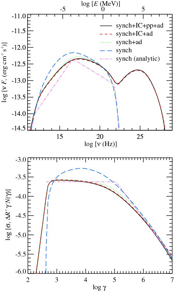
Simulated afterglow spectrum in the observer frame (top panel) and the electron distribution in the fluid frame (bottom panel) at radius r = 3.4 × 10¹⁷ cm. The particle distributions have been obtained with four different combinations of radiative and adiabatic processes. Synchrotron emission/absorption, Compton scattering, pair production/annihilation and adiabatic energy losses are indicated in the figure by the abbreviations syn, IC, pp and ad, respectively. In the simulation where only synchrotron processes are included, self-absorption heating of the electrons is not accounted for. The analytic synchrotron solution by Sari et al. (1998) is also shown in the figures. The simulation parameters are E₀ = 10⁵³erg, n₀ = 1 cm^-3, ϵ_e = 0.1, ϵ_B = 10^-3, Γ₀ = 400 and s = 2.3. The high-energy cutoff of the electron distribution has a constant value γ_max = 4 × 10⁷, and the GRB is located at a redshift z = 1. In the bottom panel, N(γ) ≡ dn/dγ is the number density of electrons per dimensionless energy interval. The distribution function has been multiplied by σ_TΔR′ to find the Thomson optical depth and by γ^s in order to visualize which electrons are cooling: a flat segment in the distribution means that the slope is the same as that of the injection function, demonstrating that the electrons are uncooled. The figure may be compared with Figs. 4 and 5 of PM09.