| Issue |
A&A
Volume 564, April 2014
|
|
|---|---|---|
| Article Number | A108 | |
| Number of page(s) | 14 | |
| Section | Astrophysical processes | |
| DOI | https://doi.org/10.1051/0004-6361/201322393 | |
| Published online | 15 April 2014 | |
Monte Carlo modelling of the propagation and annihilation of nucleosynthesis positrons in the Galaxy
1 Université de Toulouse, UPS-OMP, IRAP, 31400 Toulouse, France
e-mail: This email address is being protected from spambots. You need JavaScript enabled to view it.
2 CNRS, IRAP, 9, avenue du Colonel Roche, BP 44346, 31028 Toulouse Cedex 4, France
Received: 30 July 2013
Accepted: 23 February 2014
Abstract
Aims. We want to estimate whether the positrons produced by the β+-decay of 26Al, 44Ti, and 56Ni synthesised in massive stars and supernovae are sufficient to explain the 511 keV annihilation emission observed in our Galaxy. Such a possibility has often been put forward in the past. In a previous study, we showed that nucleosynthesis positrons cannot explain the full annihilation emission. Here, we extend this work using an improved propagation model.
Methods. We developed a Monte Carlo Galactic propagation code for ~MeV positrons in which the Galactic interstellar medium, the Galactic magnetic field, and the propagation are finely described. This code allows us to simulate the spatial distribution of the 511 keV annihilation emission. We tested several Galactic magnetic fields models and several positron escape fractions from type-Ia supernova for 56Ni positrons to account for the large uncertainties in these two parameters. We considered the collisional/ballistic transport mode and then compared the simulated 511 keV intensity spatial distributions to the INTEGRAL/SPI data.
Results. Regardless of the Galactic magnetic field configuration and the escape fraction chosen for 56Ni positrons, the 511 keV intensity distributions are very similar. The main reason is that ~MeV positrons do not propagate very far away from their birth sites in our model. The direct comparison to the data does not allow us to constrain the Galactic magnetic field configuration and the escape fraction for 56Ni positrons. In any case, nucleosynthesis positrons produced in steady state cannot explain the full annihilation emission. The comparison to the data shows that (a) the annihilation emission from the Galactic disk can be accounted for; (b) the strongly peaked annihilation emission from the inner Galactic bulge can be explained by positrons annihilating in the central molecular zone, but this seems to require more positron sources than the population of massive stars and type Ia supernovae usually assumed for this region; (c) the more extended emission from the Galactic bulge cannot be explained. We show that a delayed 511 keV emission from a transient source, such as a starburst episode or a recent activity of Sgr A*, occurring between 0.3 and 10 Myr ago and producing between 1057 and 1060 sub-MeV positrons could explain this extended component, and potentially contribute to the inner bulge signal.
Key words: astroparticle physics / gamma rays: ISM / nuclear reactions, nucleosynthesis, abundances
© ESO, 2014
1. Introduction
The 511 keV line emission from our Galaxy is unambiguously produced by low energy positrons that annihilate with electrons, but the exact origin of these positrons remains unclear. The spatial distribution of the annihilation emission was measured by several generations of gamma-ray instruments and most recently by INTEGRAL/SPI1 (Knödlseder et al. 2005; Weidenspointner et al. 2008b; Bouchet et al. 2010). It comprises faint emission from the inner part of the Galactic disk (GD) and a strong diffuse emission from the Galactic bulge (GB, which can be modelled with a narrow and a wide spheroidal Gaussian distribution with projected FWHM of ~3° and ~11° respectively, see Weidenspointner et al. 2008b). This emission is very particular, with an inferred bulge-to-disk luminosity ratio ranging from 2 to 6. None of the known Galactic astrophysical-object or interstellar-matter distributions resembles the annihilation emission distribution.
In order to explain this bulge-to-disk luminosity ratio, several authors suggested that positrons produced by supernovae in the disk could propagate far enough to annihilate in the bulge (Prantzos 2006; Higdon et al. 2009). Other authors proposed that mini-starbursts or the supermassive black hole Sgr A* produced a large amount of positrons 106 or 107 years ago, which filled the GB and are annihilating now (Parizot et al. 2005; Totani 2006; Cheng et al. 2006, 2007).
A major issue in such studies is that the propagation of positrons in the interstellar medium (ISM) is not well understood (Jean et al. 2006). In a previous detailed analysis, Higdon et al. (2009) used an inhomogeneous diffusion model, including collisional and collisionless transport of positrons, in a finely-structured ISM and found that nucleosynthesis positrons could account for all the observables of the Galactic annihilation emission. However, this model raised some criticism in the community (e.g. Prantzos et al. 2011; Martin et al. 2012). In the present paper, we would like to propose a different approach based on the theoretical investigation of Jean et al. (2009) on propagation mechanisms for positrons in the ISM. These authors show that at low energy (E ≲ 10 MeV) positrons do not interact with magnetohydrodynamic waves and propagate in the collisional mode by undergoing gyro-motion around magnetic field lines and collisions with gas particles. In such conditions, a correct treatment of positron propagation requires using representative models of Galactic magnetic field (GMF) and Galactic gas distributions. In a previous study, we performed a simulation of the propagation of positrons emitted in the decay of radioactive nuclei produced by massive stars and supernovae (26Al, 44Ti, and 56Ni) using a modified version of the GALPROP cosmic-ray propagation code (Martin et al. 2012). This code treats the transport of positrons as a diffusive process and uses two-dimensional analytical distributions of the large-scale average gas density. In this framework, we showed that it is hard to explain the morphology of the annihilation emission from radioactivity positrons, which led us to the conclusion that either an additional component is needed to explain the bulge emission or a finer modelling is required. We explored the latter option in the present work.
In this paper, we investigate the fate of positrons produced by stellar nucleosynthesis in our Galaxy with a Monte Carlo code that takes the transport of positrons in the collisional mode into account. This code simulates the injection, propagation, energy loss, and annihilation of positrons taking spatial distributions for sources, interstellar gas, and magnetic field into account. The results of the simulations allow us to derive sky maps, light curves, and spectra of the annihilation emission as functions of the sources of positrons. Section 2 describes the Monte Carlo method and the various model components. In Sect. 3, we present and discuss the results of the simulations. The simulated sky maps of the annihilation emission at 511 keV are compared to the INTEGRAL/SPI data. We show that type Ia supernovae (SNe Ia) cannot be the main source of positrons and that additional sources are needed to explain the measured disk and bulge emissions. The latter can be explained by a brief injection of a large amount of positrons in the central region of our Galaxy (e.g. in the central molecular zone) that occurred several Myr ago. In Sect. 4, we summarise our study and conclusions.
2. The Monte Carlo Galactic propagation model
The 511 keV annihilation emission mainly depends on four inputs: the properties of the ISM, the configuration of the GMF, the positron-source spatial and spectral distribution, and the positron propagation physics. In the following, we introduce the models and assumptions used for each of these inputs. We then summarise the development of the Monte Carlo simulations and explain how 511 keV intensity sky maps were generated.
2.1. Modelling the interstellar medium
We consider a static model of the ISM, which does not include any dynamic phenomena such as Galactic winds and chimneys. We divided the Galaxy into three regions: the Galactic disk (GD, R ≥ 1.5 kpc, with R the Galactocentric radius), the Galactic bulge (GB, 0.01 kpc <R< 1.5 kpc), and the Sgr A* region (R ≤ 10 pc). We then used the spatial distribution of the interstellar gas given by Ferrière (1998) and Ferrière et al. (2007) for the GD and the GB, respectively. In these models, the ISM, composed of 90% hydrogen and 10% helium, is described by five gaseous phases: the molecular medium (MM), the cold neutral medium (CNM), the warm neutral medium (WNM), the warm ionised medium (WIM), and the hot ionised medium (HIM). These models give the space-averaged density ⟨ ni ⟩ of each ISM phase i. In the GB model, the neutral (molecular and atomic) gases are confined to two structures: the so-called central molecular zone (CMZ) and a holed tilted disk. The CMZ is a 500 pc × 200 pc ellipse with a FWHM thickness of 30 pc, while the holed tilted disk is a 3.2 kpc × 1 kpc ellipse with 2.3 times the FWHM thickness of the CMZ and with a hole in the middle to leave room for the CMZ. Because the CNM and the WNM in the GB cannot be separated observationally, the GB model only gives the space-averaged density of the total (CNM + WNM) atomic gas. We denote the respective fractions of atomic hydrogen (HI) space-averaged density in the form of CNM and WNM by fCNM and fWNM. Owing to the high thermal pressure and ionisation rate in the GB (e.g. Morris & Serabyn 1996), we expect most of the atomic gas to be in the form of CNM. Indeed, thermal pressure is almost certainly above the critical pressure for warm atomic gas to exist under thermal equilibrium conditions, and while departures from thermal equilibrium may allow for some warm gas, part of it will surely be ionised by the high ionisation rate. Here, we adopted the conservative estimates fCNM = 0.7 and fWNM = 0.3. Finally, we derived the true density, ni, of each phase from its space-averaged density, ⟨ ni ⟩, using the method described in Jean et al. (2006): we multiplied its true density near the Sun ni, ⊙ by a common “compression factor”, fc, adjusted to ensure that ∑ iφi = 1 where φi = ⟨ ni ⟩ /ni is the volume-filling factor of phase i. For the ionisation fraction and the temperature of each phase, we took the mean values given in Table 1 of Jean et al. (2009).
To obtain a complete model of the Galaxy, we also modelled the interstellar gas within ~10 pc of Sgr A∗ following the recent prescription by Ferrière (2012). The ISM components of the Sgr A∗ region are geometrically identified and modelled with their thermodynamic parameters (see Table 2 of Ferrière 2012). In brief, this region can be seen as an ionised radio halo (IRH) enclosing a warm ionised central cavity, the Sgr A East supernova remnant (SNR), and a multitude of molecular structures.
We simulated positron propagation in a finely structured ISM. During propagation, a positron successively goes through clearly identified phases, and a choice had to be made about the transition from one phase to another. The Galaxy contains some regions with a well-defined structure of phases, called photodissociation regions (Tielens & Hollenbach 1985), where atomic/molecular clouds are illuminated by strong ultraviolet radiation fields and have their outer layers largely ionised. These regions are found particularly in the Galactic nucleus and in the CMZ (see e.g. Wolfire et al. 1990). Nevertheless, observations (e.g. Heiles & Troland 2003) and numerical studies (e.g. de Avillez & Breitschwerdt 2004, 2005) also show an ISM with a phase continuum, where the ISM is mixed down to relatively small scales, and not an ISM with a clear-cut separation between phases (see Vazquez-Semadeni 2009, for a review on this topic). Therefore, in this study, we considered two simplified extreme models for the Galactic ISM.
In the first model, which we called the random ISM model, each time a positron leaves an ISM phase, the next phase it enters is selected based on its filling factor. Thus, each phase with a non-zero filling factor has a finite probability of being entered by the positron. More details are given in Sect. 2.4.
In the second model, which we called the structured ISM model, the different ISM phases are related to each other everywhere in the Galaxy. The basic structure that we considered is a spherical structure with increasing temperature and ionisation fraction from the centre to the edge: a MM core, surrounded by a layer of CNM, itself surrounded by a layer of WNM, itself surrounded by a layer of WIM, with an outer envelope of HIM. In this model, a MM region cannot be found directly next to a HIM region. The volumes, hence the radii, of the different phases of this structure are determined by their respective filling factors. Each time a positron escapes such a spherical structure, another structure is generated. The calculation of the exact dimensions of the spherical structure is presented in Sect. 2.4.
These two representations are limiting cases of the layout and ordering of the ISM, and we discuss their respective impact on the results.
2.2. Modelling the Galactic magnetic field
The structure of the GMF is often described with two components: the regular GMF and the turbulent GMF. These two components are probed with measurements of the total and polarised synchrotron emission and Faraday rotation of pulsars and extragalactic sources. Recent studies (Sun et al. 2008; Sun & Reich 2010; Jansson & Farrar 2012) tend to show that the regular GMF could be made up of a disk field and a halo field component.
We modelled the disk regular component using the model of Jaffe et al. (2010), which is a parametric two-dimensional coherent spiral arm magnetic field model that provides predictions for observables, such as synchrotron intensities and Faraday rotation measures. To obtain a complete three-dimensional model of the regular GMF, we assumed that the spiral field strength decreases exponentially above and below the Galactic plane with a scale height of 1 kpc (see e.g. Prouza & Šmída 2003; Sun et al. 2008).
The configuration of the halo regular field is even more uncertain than that of the disk regular field. It has been suggested that this halo component is a poloidal field with a dipole shape (see Han 2004, for a review). Based on this dipole morphology, Prantzos (2006) argues that the positrons produced in the disk could be transported into the bulge, thereby explaining the atypical 511 keV emission distribution. However, the recent analysis by Jansson & Farrar (2012) found support for the presence of an X-shape magnetic field in the Galactic halo, as could be expected from observations of X-shape fields in external spiral galaxies seen edge-on (see e.g. Krause 2009). Due to the uncertainties in our knowledge of the halo GMF, we tested three configurations of the halo regular field: no halo field, the dipole field as described in Prouza & Šmída (2003), and the X-shape field as described in Jansson & Farrar (2012). The three configurations will be respectively denoted by N, D, and X in the tables.
The status of the GMF in the Sgr A* region is rather uncertain and has never been thoroughly reviewed. In this work, we assumed that the magnetic field in all the diffuse and ionised regions near Sgr A* is perpendicular to the Galactic plane and has a strength of 0.1 mG (see Ferrière 2012, for a description of the Sgr A* region). We then assumed that the magnetic field in the dense and neutral regions is oriented along the long dimension of the local clouds and has a strength of 1 mG (Ferrière 2009, and references therein).
In addition to the regular component, we modelled the turbulent GMF using the plane wave approximation method described by Giacalone & Jokipii (1994). We assumed that magnetic field fluctuations follow a Kolmogorov spectrum and have a maximum turbulent scale  in the range 10−100 pc in the hot and warm ISM phases and 1−10 pc in the cold neutral and molecular phases of the ISM. In previous studies of the positron propagation (Prantzos 2006; Jean et al. 2009), the ratio δB/B0 was assumed to be constant throughout the Galaxy. Here, we allowed this ratio to vary in space in the GD with δB/B0 increasing smoothly from one in interarm regions to two along the arm ridges (see Jaffe et al. 2010). We set this ratio to one in the GB.
2.3. Modelling the positron sources
The most promising source of Galactic positrons is the β+-decay of unstable nuclei synthesised in massive stars or supernovae. The reasons for this are that (a) some radio-isotopes emitting positrons, such as 26Al and 44Ti, have been observed within the Galaxy via the gamma-ray or X-ray lines that accompany their decay; (b) the observed or theoretical radio-isotope yields can supply positrons so as to feed the 511 keV luminosity derived from INTEGRAL observations; and (c) the positrons from radioactivity are released in the ISM with energies that are on average lower than 1 MeV, which agrees with the constraints obtained by Beacom & Yüksel (2006) and Sizun et al. (2006). In the following, we make a short summary of Sect. 4 of Martin et al. (2012), who present all of the properties of each source studied here, and we highlight the slight differences with their work. We assumed a steady-state Galactic production rate of all the following radioisotopes.
The radio-isotope 26Al decays with a lifetime of ~1 Myr, emitting a gamma photon at 1809 keV and a positron 82% of the time. Its spatial distribution is strongly correlated with the free-free emission from HII regions surrounding massive stars (Knödlseder et al. 1999), confirming that its nucleosynthesis is linked to massive stars. We therefore used the free-electron spatial distribution (NE2001 model) of Cordes & Lazio (2002) for the distribution of 26Al. More specifically, we adopted the thin disk and spiral arm components of the NE2001 model for the disk massive stars. In the following, we call this component the star-forming disk (SFD) component. We also took the Galactic center (GC) component from the NE2001 model into account, since roughly 10% of the massive stars could be formed in the inner stellar bulge (R< 0.2 kpc), following the argument given by Higdon et al. (2009). This component is quite similar to the CMZ defined in Ferrière et al. (2007), so in the following we call it the CMZ component and assign it 10% of the 26Al positrons. Thanks to the very long decay lifetime of 26Al, positrons are very likely injected into the ISM with their original β+-spectrum with a mean energy of ≃0.45 MeV. The steady-state Galactic production rate of 26Al positrons can be derived from the present-day mass equilibrium of 26Al in the Galaxy. Here, we took the value of ≃(2.8±0.8) M⊙ (Diehl et al. 2006), but we also took note of the estimate of (1.7−2.0±0.2) M⊙ derived by Martin et al. (2009). With a β+-decay branching ratio of 82%, we obtain a positron production rate ≃(3.2 ± 0.9) × 1042 e+ s-1.
The radio-isotope 44Ti decays with a lifetime of ≃85 yr into 44Sc, which in turn decays very quickly into 44Ca, emitting a positron 94% of the time. 44Ti is mainly synthesised during core-collapse supernova explosions (ccSNe) of massive stars. Thus, we used the same spatial distribution (SFD+CMZ) as for 26Al for the spatial distribution of 44Ti. The 44Ti positrons have to travel across stellar ejecta before entering the ISM, but because of the intermediate decay lifetime of the radioisotope, we assumed that 44Ti positrons are also released into the ISM with their original β+-spectrum with a mean energy of ≃0.6 MeV. Based on the production rate of 56Fe and the measured solar (44Ca/56Fe)⊙ ratio (see Prantzos et al. 2011), the positron production rate from 44Ti is ≃3 × 1042 e+ s-1. We assumed an uncertainty range of ±50% on this positron injection rate to reflect the uncertainties on the 44Ti production rate.
The radio-isotope 56Ni decays with a lifetime of ≃9 days into 56Co, which in turn decays with a lifetime of ≃111 days into 56Fe, emitting a positron 19% of the time. The 56Ni is synthesised during ccSNe and thermonuclear supernova explosions (SNe Ia), but SNe Ia are by far the dominant source of positrons thanks to their higher iron yield per event and their much higher positron escape fraction from the ejecta (Martin et al. 2012). 56Ni therefore follows the time-averaged spatial distribution of SNe Ia in the Galaxy. Sullivan et al. (2006) show that the spatial distribution of SNe Ia is a combination of the young stellar populations and the stellar mass distributions. We thus assumed that a distribution of old/delayed SNe Ia follows an exponential disk (ED) with a central hole plus an ellipsoidal bulge (EB), both components tracing the stellar mass (see Sect. 6.1 of Martin et al. 2012). Then, a population of early/prompt SNe Ia is associated with the SFD. We do not consider early/prompt SNe Ia occurring in the CMZ because the uncertainties on the SNe Ia rate in this region are large (see for instance Schanne et al. 2007). We discuss that point in Sect. 3.3.
56Ni and 56Co have very short lifetimes and their positrons are injected directly into the ejecta of the supernova, very likely experiencing strong energy losses before reaching the ISM. Therefore, the β+-spectrum of 56Co positrons is altered in comparison with the original β+-spectrum. Using the method of Martin et al. (2010, Sect. 5), we computed some altered β+-spectra for three escape fractions from the ejecta: 0.5%, 5% and 10%. We chose these three values because they lie in the range of the estimations of several studies (see Chan & Lingenfelter 1993; Milne et al. 1999, for instance). The calculated altered β+-spectra have a mean energy of 105, 175, and 205 keV for the escape fraction of 0.5%, 5%, and 10%, respectively. These values are very different from the mean energy of ~0.6 MeV of the unaltered β+-spectrum. Using the same computation as Martin et al. (2012, Eq. (1)) for the SN Ia occurrence rate, we derived a positron injection rate of 4.45, 4.17, and 6.0 × 1042 e+ s-1 for the ED, the EB, and the SFD components, respectively. These values are given for a typical 56Ni yield of 0.6 M⊙ per event, a β+-decay branching ratio of 19% and a positron escape fraction of 5% from the stellar ejecta2.
2.4. Modelling the propagation physics
After being released in the ISM by their parent radio-isotope, positrons propagate within the Galaxy, slowing down until they annihilate directly with an electron or via positronium (Ps) formation. The Ps is the bound state of a positron with an electron, which is formed 25% of the time in the para-Ps state and 75% of the time in the ortho-Ps state. The ortho-Ps decays in 140 ns into three photons of energies totalling 1022 keV and the para-Ps decays in 0.125 ns into two photons of 511 keV contributing to the 511 keV γ-ray, which is also produced by the direct annihilation of a positron with an electron (Guessoum et al. 1991, 2005).
A positron can propagate in the Galaxy under two different regimes: collisional or collisionless (Jean et al. 2009). In the collisional regime, the positron has a ballistic motion; it propagates spiralling along the Galactic magnetic field lines undergoing pitch angle scattering due to collisions with gas particles. In the collisionless regime, the positron scatters off magneto-hydrodynamic waves associated with interstellar turbulence. Jean et al. (2009) show that positrons could only interact with the Alfvén wave turbulent cascade in the ionised phases of the ISM, but the anisotropy of magnetic perturbations very likely makes this transport mode inefficient (see also Yan & Lazarian 2002). In this study, we only considered the collisional transport mode. We considered continuous energy-loss processes (Coulomb collisions, inverse Compton scattering, synchrotron), binary interactions with atoms and molecules (ionisation and excitation), and pitch angle scattering as described in Sect. 3 of Jean et al. (2009).
A positron travels through the different phases of the ISM. In the random ISM model (as defined in Sect. 2.1), we assumed that the positron leaves a given phase when the distance travelled inside this phase is greater than a certain distance d that is derived randomly from the probability density function of the distances that a particle can cross through a sphere of diameter di in a straight line: 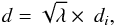 (1)where λ is a random number uniformly distributed between 0 and 1, and di is selected randomly in the typical size ranges of the considered ISM phase (see Table 4 of Jean et al. 2006). The new ISM phase i is chosen randomly according to the probability
 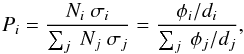 (2)where σi is the cross section of the spherical region of phase i (
 ) and Ni is the number density of spherical regions of phase i (Ni ∝ φi/Vi, with
  the volume of phase i).
In the structured ISM model, the positron is injected at the surface of a new spherical structure. The radius of this structure, rsphere, is selected randomly between 50 and 100 pc, which roughly corresponds to the observed radii of evolved supernova remnants or the maximum sizes of the HIM (see Table 4 of Jean et al. 2006). In the CMZ, the radius rsphere is selected randomly between 15 and 30 pc. With this range of rsphere and a molecular gas filling factor φMM ≃ 10 − 12%, we find that the innermost molecular region has a radius ≃7–15 pc, consistent with the observed sizes of molecular clouds in the CMZ (see e.g. Oka et al. 1998).
At a given Galactic location, each phase filling factor φi is supposed to be known. In accordance with these filling factors, we fill the structure, from the outer surface to the centre, with ISM phases of decreasing temperature and ionisation fraction. The radius of shell s is thus given by 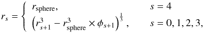 (3)where s = 0,1,2,3,4 refers to the MM, CNM, WNM, WIM, HIM, respectively. The ISM phases are thus fixed. This model locally reproduces the filling factors and specific transitions between the ISM phases. The positron is free to travel inside this onion skin structure until it escapes or annihilates. When the positron escapes, a new spherical structure is generated, tangent to the previous spherical structure, with the new local filling factors of the different ISM phases.
2.5. Summary of a Monte Carlo simulation
In the Monte Carlo code, the positron is first injected randomly in the Galaxy, at a certain location depending on the initial spatial distribution of its radioisotope, with a certain energy selected randomly from the original or altered β+-spectrum of the radioisotope (see Sect. 2.3). We assume that the positron is released in the HIM with the direction of its initial velocity chosen randomly according to an isotropic velocity distribution. Then, the positron propagates in the collisional regime following the turbulent and regular GMF lines (see Sect. 2.2), experiencing continuous energy losses, pitch angle scattering, and potentially binary interactions in the ISM phase in which it is travelling (see Appendix B of Jean et al. 2009, to have a complete overview of the Monte Carlo algorithm). During its lifetime, the positron changes ISM phase as described in Sect. 2.4. We emphasise that the collisional transport of the positron is truly inhomogeneous given that each ISM phase has its own regular magnetic field as a function of the current Galactic location and its own magnetic turbulence properties (see Sect. 2.2).
The tracking of a positron stops when it annihilates in-flight or when its energy drops below a threshold energy that we set to 100 eV, below which the distance travelled by a positron is short compared to the size of any phase, except in the HIM where we nevertheless keep on modelling the transport of the thermalised positrons. Owing to the very low density of the HIM, thermal positrons are very likely to escape the HIM and then to annihilate in a surrounding denser medium. Once the positron has annihilated, we store its final position, propagation time, energy, and ISM phase. The simulation can also stop when the positron escapes the Galaxy, i.e., when the positron goes higher than 5 kpc on either side of the Galactic plane or beyond 20 kpc in Galactocentric radius.
Bulge, disk, and total 511 keV annihilation fluxes (in ph cm-2 s-1) for 26Al, 44Ti, and 56Ni positrons.
By simulating a great number of positrons (N0 = 105), we can estimate the steady state intensity spatial distribution at 511 keV. For a given source m (defined by a radio-isotope, together with one of its spatial components), a given halo magnetic field configuration and a given escape fraction for SN Ia positrons, storing the final parameters allows us to calculate the steady state 511 keV total annihilation flux: 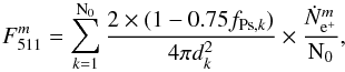 (4)where dk and fPs,k represent the distance of the annihilated positron k to the Sun, and the total Ps fraction of the ISM phase in which positron k annihilates (calculated from Guessoum et al. 2005).
  is the positron production rate for source m, reduced by the positron escape fraction. To obtain the total annihilation emission flux due to all the nucleosynthesis positrons, we just need to sum over all sources m:
 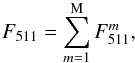 (5)with M = 7 as the number of possible sources (m = 26Al + CMZ, 26Al + SFD, 44Ti + CMZ, 44Ti + SFD, 56Ni + EB, 56Ni + ED, 56Ni + SFD).
3. Results of the simulations and discussion
The numerical model described above allowed us to compute the annihilation emission associated with each radioisotope and for each spatial component of its source distribution. The predicted annihilation emission could strongly depend on two poorly known parameters: the halo magnetic field configuration and the SN Ia escape fraction fesc for 56Ni positrons (see Sects. 2.2 and 2.3, respectively).
In Sect. 2.1, we introduced two representations for the distribution of phases in the ISM. All the simulations discussed below were performed for both representations and turned out to yield very similar results in terms of positron transport and the morphology of the annihilation emission. Therefore, for these aspects, only the results corresponding to the random ISM model will be presented below. The only difference in the results obtained with the two prescriptions for the ISM lies in the annihilation phase fractions, and this is discussed in Sect. 3.5, where both sets of results will be shown.
We thus carried out a total of 39 simulations (=3GMF × (226Al + 244Ti + 356Ni × 3fesc)) of 105 positrons corresponding to all possible combinations of halo GMF configuration, source, and fesc. These simulations give nine (=3GMF × 3fesc) different total annihilation emission sky maps due to all nucleosynthesis positrons. In Table 1, we present, for each positron source and each halo GMF configuration, the 511 keV annihilation flux in the GB, the GD, and the entire Galaxy. The bulge-to-disk flux ratios and the fractions of positrons that escape from the Galaxy are also indicated.
In the following, we first present the main results for the transport of positrons in each simulation, in particular their ranges and life times. Then, we present the predicted annihilation emission for each individual positron source and for all nucleosynthesis positrons together, depending on the GMF configuration. These models are then compared to recent measurements of the 511 keV emission by the SPI spectrometer onboard the INTEGRAL mission, which shows that the observed emission cannot be completely accounted for. We therefore discuss in a subsequent part the possible contribution of a transient source at the GC to the 511 keV emission. Finally, we present the distribution of the positron annihilation over the different ISM phases and compare it to the spectrometric constraints.
3.1. Positron ranges and life times
The numerical model allowed us to track the distance travelled by positrons in our Galaxy models. Two important results consistently emerged from our simulations. First, for each positron source and for each halo GMF configuration, only a small fraction of positrons escape the Galaxy (≲7%; see Table 1). In the case of an X-shape GMF, up to 30% of the positrons produced by massive stars in the CMZ can escape the Galaxy, but these positrons represent only 10% of the Galactic production by massive stars (see Sect. 2.3). Second, whatever the positron source or the halo GMF configuration, positrons that do not escape the Galaxy only travel on average a distance ~1 kpc from their injection site.
The travelled distance varies slightly with the halo GMF configuration and positron production sites. For instance, positrons produced in the very dense CMZ annihilate quickly and only travel about 150–300 pc, except in the simulation with the X-shape halo GMF where they travel on average 600 pc. This is because the vertical magnetic field lines of the X-shape halo GMF near the GC allow positrons to quickly escape the Galactic plane. The travelled distance also slightly varies with the initial energy of positrons. For instance, 56Ni positrons from SNe Ia occurring in the SFD travel on average ~600–700 pc, while the more energetic massive-star positrons (26Al and 44Ti positrons) produced in the SFD travel on average ~0.9–1.1 kpc. But generally, nucleosynthesis positrons do not travel too far away from their birth places. This strongly explains that the morphologies of the 511 keV emission sky maps are very similar, as presented and discussed in Sect. 3.3, and that our simulated 511 keV spatial distributions closely reflect the spatial distributions of the positron sources.
The reasons for nucleosynthesis positrons not travelling far away from their birth places are (a) the initial positron energies are only a few 100 keV and not ~1 MeV as usually assigned in previous studies (e.g. Prantzos 2006) and (b) here, positrons are injected in a realistic ISM where the true density of each ISM phase is taken into account, which also reduces the propagation distances. This is a stringent constraint. For instance, a positron entering the CNM near the Sun will travel in a medium with a true density ≃40 cm-3 contrary to the local CNM space-average density ≃0.3 cm-3 given by the model of Ferrière (1998).
Accordingly, the average lifetime of nucleosynthesis positrons also depends slightly on the initial energy of positrons, the halo GMF configuration, or the positron production sites. Regardless of the halo field configuration and the escape fraction, the SN Ia positrons slow down in ~(5–8) × 105 years when they are produced in the EB or the ED component, which mainly consists of tenuous Galactic regions (GB). In contrast, when they are produced in the denser regions of the SFD, they slow down in only ~(2–4) × 105 years. The more energetic massive-star positrons slow down on average in ~(6–7)×105 years when they are produced in the SFD. However, their mean lifetime depends on the halo GMF configuration when they are produced in the CMZ. With a dipole halo field, they slow down in only ~1 × 10⁵ years, whereas they slow down on average in ~7 × 10⁵ years with a X-shape halo field.
The simulations cannot explain the large bulge-to-disk (B/D) flux ratio of ~1–3 derived from INTEGRAL/SPI observations (Knödlseder et al. 2005). We only obtain B/D flux ratios of ~0.05 for comparison. The reason is that the nucleosynthesis positrons produced in the GD cannot reach the GB. Our simulations thus do not support the scenario proposed by Prantzos (2006), who suggests that SN Ia positrons produced in the GD could be transported via a dipole GMF into the GB. However, the dipole halo field could play an important role confining positrons produced in the CMZ, as we see in Sect. 3.3.
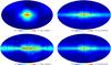 |
Fig. 1 Simulated all-sky maps of the 511 keV intensity distribution (in ph cm-2 s-1 sr-1) for 56Ni positrons with the dipole halo field configuration and an SN Ia escape fraction of 5%. The maps correspond to the 511 keV emission of positrons produced in the ellipsoidal bulge component (top left), the holed exponential component (top right), the SFD component (bottom left), and the entire Galaxy (by summing the three previous all-sky maps; bottom right). |
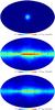 |
Fig. 2 Simulated all-sky maps of the 511 keV intensity distribution (in ph cm-2 s-1 sr-1) for 26Al and 44Ti positrons with the dipole halo field configuration. From top to bottom, the maps correspond to the 511 keV emission of positrons produced in the CMZ component, in the SFD component, and in the entire Galaxy (by summing the two above all-sky maps). |
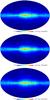 |
Fig. 3 Simulated all-sky maps of the 511 keV intensity distribution (in ph cm-2 s-1 sr-1) for all nucleosynthesis positrons, with an SN Ia escape fraction of 5% for 56Ni positrons, and for the three halo GMF configurations. From top to bottom, the maps correspond to no halo field, the dipole field, and the X-shape field. The sky maps have been put on the same intensity logarithmic scale. |
3.2. 511 keV annihilation emission
Unless stated otherwise, all the results presented below were obtained for a dipole halo GMF and an SN Ia escape fraction fesc = 5%. Figures 1 and 2 show the all-sky intensity maps of the annihilation emission for 56Ni positrons and 26Al+44Ti positrons, respectively. (We present the cumulated emission from positrons from 26Al and 44Ti because their respective contributions have the same morphology, see Fig. 5, because they have the same progenitors and similar injection energies.) In these figures, the 511 keV intensity distribution of each spatial component of the source distribution is given before showing the total 511 keV intensity distribution. Figure 3 shows the 511 keV intensity distribution for the annihilation of all nucleosynthesis positrons for each halo GMF configuration and with fesc = 5%. The longitude profiles of these sky maps are presented in Fig. 4, while Fig. 5 shows the longitude profile for each positron source and each fesc, in the case of a dipole halo GMF configuration.
The halo GMF configuration has very little effect on the 511 keV emission morphology, as illustrated by Fig. 3. The longitude profiles (Fig. 4) confirm this trend and underline that the 511 keV emission spatial distribution reflects the positron source spatial distribution. We present in this figure the longitude profile of the 511 keV emission corresponding to the case where positrons annihilate at their sources without propagation. This profile is very similar to the three other profiles, which is explained by the fact that nucleosynthesis positrons do not propagate very far away from their birth places.
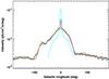 |
Fig. 4 Longitude profiles of the 511 keV emission of all nucleosynthesis positrons, with an SN Ia escape fraction of 5% for 56Ni positrons and for the three halo GMF configurations (corresponding to the maps in Fig. 3, with an integration range | b | ≤ 10°): no halo field (blue curve), dipole field (black curve), and X-shape field (green curve). The red curve corresponds to the longitude profile of all nucleosynthesis positrons in the absence of propagation, assuming they annihilate in a medium with a positronium fraction of 0.95. The cyan curve corresponds to an analytical model obtained by model fitting to INTEGRAL/SPI observations and given only over the longitude range where data are constraining (see text). The difference in normalisation shows that the positron injection rates used in the model are overestimated by a factor ~2. |
For SN Ia positrons, the escape fraction has very little impact on the distribution of the resulting 511 keV intensity sky maps because of slight differences in the energy spectra (see Sect. 2.3). The main difference resides in the normalisation of the 511 keV intensity map, which depends on the positrons injection rate in the Galaxy (see Fig. 5). This can also be seen in Table 1, in which the total 511 keV Galactic flux of each simulation is quasi-proportional to its fesc, for a given GMF configuration.
In Fig. 3, the bulk of the 511 keV emission due to all nucleosynthesis positrons is concentrated in the longitude range | l | ≤ 50°, in agreement with the extent measured by INTEGRAL/SPI (Weidenspointner et al. 2008a; Bouchet et al. 2010). The sky maps have a highly-peaked 511 keV emission from the inner bulge, mostly due to the annihilation of 26Al and 44Ti positrons produced in the CMZ. The main difference between the three GMF models comes from this emission component. The 511 keV intensity in the inner bulge is ~1.25 and ~2.5 times higher in the Galaxy model with a dipole halo GMF than in a Galaxy without a halo GMF and with an X-shape halo GMF, respectively.
Another noteworthy feature concerning the morphology is the asymmetric emission from the GD. This is due to the annihilation emission of positrons produced in the SFD (see the same feature in Figs. 1 and 2). The longitude extent of their GD emission is larger towards negative longitudes than toward positive longitudes. Most of the emission comes from between 0 to l ≃ − 75° at negative longitudes, whereas it comes from between 0 to l ≃ 45° at positive longitudes (see also Figs. 4 and 5). This occurs because the line of sight towards l ≃ − 75° follows the positron-producing Sagittarius-Carina arm from the NE2001 model over a long distance (see Fig. 6 of Cordes & Lazio 2002).
3.3. Comparison to the INTEGRAL/SPI data
We compared the simulated sky maps to INTEGRAL/SPI observations by a model fitting method, in which a sky model convolved by the instrument response function is fitted to the data, along with a model of the instrumental background. The main results of a model fitting are the maximum likelihood ratio (MLR), which basically allows different models to be compared, and the fit parameters, which in the present case correspond to the rescaling of the model required for a better match to the data (see Knödlseder et al. 2005, for further information on the model-fitting procedure). In this study, we used public data of the spectrometer SPI taken between December 9, 2002 and August 20, 2010. We performed the model fitting analysis in a 5 keV wide energy bin centred at 511 keV, including the Crab and Cygnus X-1 as point sources for the sake of completeness. We then compared our results to a phenomenological analytical model.
For the latter, we used the analytical model from Weidenspointner et al. (2008b). It is composed of a small spheroidal Gaussian superimposed on a large spheroidal Gaussian to account for the bulge emission (the inner and outer bulges, respectively), and a holed exponential disk like the one described by Robin et al. (2003) for the young stellar population to represent the GD emission. We updated the spatial components (widths and positions of the Gaussians, scale length, and height of the disk) of their model from a fit to our data set. In contrast to the original model, we used a large Gaussian that was slightly shifted toward negative longitudes (~ − 1°) because this improves the fit to the data (see also Skinner et al. 2010). In the following, this best-fit updated analytical model will be referred to as UW and its inner and outer spheroidal Gaussian components as IB and OB, respectively. The longitude profile of this model is presented in Fig. 4. It is plotted for the inner Galactic region alone (| l | ≥ 50°) because it is currently unconstrained outside of this range (Bouchet et al. 2010).
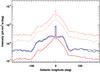 |
Fig. 5 Longitude profiles of the 511 keV emission (integration range | b | ≤ 10°) from 26Al (blue curve), 44Ti (black curve), and 56Ni (red curves) positrons, with an SN Ia escape fraction of 0.5% (solid curve), 5% (dotted curve), and 10% (dashed curve) for 56Ni positrons, in the case of a halo dipole field configuration. |
Looking at Fig. 4, it first appears that the normalisation of our models is too high. Reducing the positron injection rates used as a base case by a factor ~2 would bring the predictions in line with the observations (a more quantitative discussion is given below). Nevertheless, it is obvious that none of our intensity sky maps, regardless of the halo GMF configuration, can fully account for the 511 keV emission. Renormalising the intensity would make it possible to account for the GD emission in the | l | = (10 − 50)° range, but in any case would not account for the full bulge emission. An additional source is thus necessary to explain the bulge emission, especially the outer bulge. However, in contrast to our previous study in Martin et al. (2012), we observe a strong and sharp intensity peak at the position of the GC region, which seems to match the inner bulge component. The reason is that we carefully modelled the CMZ and took the massive-star positrons produced there into account. Depending on the halo GMF configuration, the very dense CMZ is a major trap for (a) positrons that are directly injected in the CMZ and (b) positrons that are channelled into it (see the central intensity peak for each source in Fig. 5).
We confirmed by model fitting that our simulated 511 keV Galactic distributions can account for the observed GD emission as satisfactorily as the disk component of the best-fit analytical model. Fitting to the data the IB and OB components of the best-fit analytical model, together with our simulated 511 keV intensity distributions, yields the results presented in Table 2, for fesc = 5% and the three halo GMF configurations. (The fits for the other values of fesc give similar MLR but with different scaling factors.) Statistically, our simulated emission models describe the measured disk emission as well as the young stellar population disk of the analytical best-fit model. The maximum difference in MLR is about six, which is not significant. Therefore, the fit to the data does not allow us to constrain the halo GMF configuration. Moreover, regardless of the halo field, the fitted fluxes of our simulated disk models are similar. The scaling factors for all our models are about 0.5. This means that the positron production rate of one or several radioisotopes has perhaps been overestimated (see Sect. 2.3 for the uncertainties).
Results of the fits of our simulated 511 keV emission spatial distributions due to all nucleosynthesis positrons, with an SN Ia escape fraction of 5% for 56Ni positrons, and for the three halo GMF configurations, to about 8 years of INTEGRAL/SPI observations.
Results of the fits of our simulated 511 keV emission spatial distributions to about 8 years of INTEGRAL/SPI observations.
The major difference between these different model fits lies in the fitted flux for the IB component, because our simulated 511 keV intensity distributions already include a strong peak at the Galactic centre position, although at different levels depending the GMF. The IB component emission for a dipole halo field is ≃33% and ≃40% lower than for a no halo field and an X-shape halo field, respectively. The reason is that the dipole halo field confines positrons produced in the CMZ and makes them annihilate quickly, compared to the other two configurations (see Sect. 3.1). Moreover, the dipole halo field is more likely to channel positrons produced by SNe Ia in the GB towards the CMZ. Thus, with the dipole halo GMF, the inner bulge emission in our model is more intense, and the analytical IB component superimposed on it needs to have a lower flux to bring the total emission up to the observed level.
In summary, our fits showed that the data cannot constrain the halo GMF configuration or the SN Ia escape fraction because of the strong similarities between our different sky maps.
We then sought to independently estimate the contribution of each positron source to the Galactic 511 keV emission, and even beyond the contribution of some of their source components. To do this, we carried out a series of fits to the data with different emission models and/or combinations of models derived from the simulations with a dipole halo GMF. The results of the fits are shown in Table 3. For massive-star positrons, we did not make any distinction between 26Al and 44Ti because of their very similar intensity distributions. We thus used 26Al models alone and considered the more uncertain 44Ti as a possibility for increasing the intensity by a factor of up to 2 (see Sect. 2.3).
In a first step, we fitted to the data only one emission model related to positrons from one radioisotope, all source components included. The fits are not good at all, as illustrated by the longitude profiles of Fig. 5. In a second step, we added the analytical OB component to the nucleosynthesis positron all-sky models. Adding the OB component significantly improves the fits. The 511 keV all-sky emission from 26Al positrons combined with the analytical OB component is able to explain the morphology of the observed all-sky 511 keV emission as satisfactorily as the best-fit analytical model (MLR = 2758 and 2766, respectively). In contrast, the 56Ni-only emission model with the OB does not give such a good fit to the data (MLR = 2743). This can be easily understood from Fig. 5: the intensity ratio between the emission peak and the underlying disk is only ~2 for 56Ni positrons while it is ~4 for massive-star positrons. The latter ratio is closer to the ratio of the best-fit analytical model, which is ~5. The 26Al positron emission model and the OB can explain the morphology of the 511 keV emission, but the 26Al positron emission is rescaled in the fit by a factor of 3.6 ± 0.3. Adding the contribution from 44Ti positrons to this model could not account for this scaling factor, even with the upper limits of the positron production rate by 26Al and 44Ti. Therefore,56Ni positrons seem to be needed to quantitatively explain the observed 511 keV emission in the disk and the inner bulge.
To demonstrate this, in a last step, we fitted a model made of three components: (a) the emission of 26Al positrons produced in the CMZ, (b) the emission of 26Al positrons produced in the SFD added to the emission of all 56Ni positrons, and (c) the OB component. This global model describes the data as satisfactorily as the UW model (MLR = 2759.8). We obtained scaling factors of 3.4±0.6 and 0.62±0.06 for the CMZ 26Al positron model and the (SFD 26Al+56Ni) positron model, respectively. The latter scaling factor suggests that one or several positron sources in the disk were overestimated. For instance, assuming that our estimate for the 26Al positrons injection rate is correct, fesc ≃ 2.5% would be sufficient to quantitatively explain the observed GD 511 from 26Al and 56Ni alone. Considering a contribution from 44Ti would push the escape fraction even lower. Thus, it seems that the 511 keV emission from the GD could be explained both morphologically and quantitatively from all radio-isotopes positrons. However, the 511 keV emission from the CMZ requires a larger correction factor of 3.4±0.6 to account for the inner bulge emission. One possibility would be that massive stars in the CMZ are either more numerous than assumed here (10% of all massive stars; see Sect. 2.3) or more efficient at producing positrons, for instance, because of a more favourable IMF. However, we should keep in mind that the amount of 26Al is constrained by the detection of the 1.8 MeV γ-ray line (see e.g. Martin et al. 2009). Another possibility would be to consider a contribution of SNe Ia in the CMZ. Assuming that 10% of the prompt SNe Ia occur in the CMZ as for massive stars (which roughly corresponds to the prompt SN Ia rate derived in the CMZ by Schanne et al. 2007 and Higdon et al. 2009), we obtain a positron production rate of ≃6 × 1041 e+ s-1. Added to the positron production rate of 26Al positrons in the CMZ (≃3.2 × 1041 e+ s-1), this contribution could explain the factor of ~3 needed to account for the CMZ emission. Taking a contribution from 44Ti positrons in the CMZ into account would imply a lower escape fraction of SN Ia positrons of fesc ≤ 2.5%, or a fraction of prompt SNe Ia occurring in the CMZ reduced by ~2.
Finally, one should note that the above discussion holds for the dipole field model. The fit of the three-component model for the simulations with the two other halo GMF configurations gives similar MLRs (MLR = 2760 and 2762.9 with no halo field and the X-shape halo field, respectively). However, in both cases, the emission model of 26Al positrons produced in the CMZ needs a higher scaling factor than found with the dipole halo GMF (5.8 and 10 with no halo field and the X-shape halo field, respectively). The problem of the renormalisation of the 26Al CMZ component thus becomes more acute, which opens the possibility of an additional contribution to the inner bulge emission on top of stellar nucleosynthesis.
In all cases, the positrons produced by steady state nucleosynthesis cannot explain the emission of the outer bulge detected by INTEGRAL/SPI. One possibility recently investigated is that of dark matter scattering (Vincent et al. 2012; note that this work did not include propagation that could modify the morphology of their 511 keV emission), which seems to confirm earlier predictions (see e.g. Boehm et al. 2004). In the following section, we present a possible alternative explanation based on a transient phenomenon.
As a last note on these considerations, and connected to what follows, we would like to emphasise that the separation of the observed bulge emission into an outer and an inner component is somewhat artificial and comes primarily from the choice of the functions used to model the observations (Weidenspointner et al. 2008b). In the above paragraphs, we showed that the outer bulge emission cannot be reproduced and that the predicted inner bulge emission may also be short of what is measured. Actually, it may well be that a single component could account for both these two shortcomings at the same time (such as the transient component discussed below).
3.4. Transient source
None of the positron radioactive sources, when studied in a steady state way, can explain the ≃10° extended emission arising from the GB. In the following, we show that a 511 keV emission produced by a transient source injecting a large number of positrons and seen at a particular moment after this event, hereafter called outburst, could explain the extended 511 keV emission from the GB. Only preliminary results are presented here to illustrate the idea. A more detailed study with direct comparisons to the data via model fitting will be performed elsewhere.
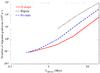 |
Fig. 6 Number of positrons injected at the outburst in the CMZ, which makes it possible to reproduce a 511 keV flux of 5 × 10⁻⁴ ph cm-2 s-1 outside the CMZ (R> 200 pc) today, as a function of time since outburst. The curves are shown only over the time intervals when the flux inside the CMZ (R< 200 pc) is below the observed 1.5 × 10⁻⁴ ph cm-2 s-1 (hence the truncations of the left parts). The solid red, dotted black, and dashed blue curves correspond to the simulations carried out with a X-shaped, dipole, and no halo GMF configurations. |
We carried out simulations of the propagation of a given amount of 26Al positrons produced in the CMZ during the outburst for the three halo GMF configurations. We calculated 511 keV light curves from the inner bulge (R< 200 pc) and the outer bulge (R> 200 pc), and compared them with the flux of the best-fit analytical model for two regions (≃1.5 × 10⁻⁴ and ≃5 × 10⁻⁴ ph cm-2 s-1 in the inner and the outer bulge, respectively; see Table 2). The 511 keV flux is computed by considering the annihilation from Ps formed in flight and from thermalised positrons. Positrons that become thermalised can survive for several Myr in a tenuous plasma, and this is the case for the ionised ISM phases in the GB. The fractions of Ps formed in flight and the annihilation rates were taken from Guessoum et al. (2005).
Figure 6 shows the number of positrons injected at the outburst that is necessary to obtain a flux ≃5 × 10⁻⁴ ph cm-2 s-1 outside the CMZ, as a function of time after the outburst. The curves are shown only over the time interval when the flux in the inner bulge is not greater than ≃1.5 × 10⁻⁴ ph cm-2 s-1.
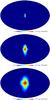 |
Fig. 7 Simulated all-sky maps of the 511 keV intensity distribution for an outburst of 26Al positrons in the CMZ for the X-shape halo field configuration (in ph cm-2 s-1 sr-1). From top to bottom, the maps correspond to the average 511 keV emission between 0 and 1 × 10⁵ yr, 5 × 10⁵ and 6 × 10⁵ yr, 1.9 × 10⁶ and 2 × 10⁶ yr after the outburst, respectively. The number of positrons injected into the outburst is 1058. |
We show that a very recent outburst that occurred less than 3 × 10⁵ yr ago is ruled out because the 511 keV emission remains too intense in the inner bulge compared to observations. However, regardless of the halo GMF configuration, an outburst occurring between ~2 and ~10 Myr ago could explain the 511 keV flux outside the inner bulge. The number of positrons injected by this outburst ranges between 1058 and 1060 positrons. The X-shape halo GMF requires the lowest number of injected positrons to account for the outer bulge emission, regardless of the time elapsed since the outburst. This is because the vertical magnetic field lines of the X-shape field allow positrons to escape the CMZ quickly, so that, the flux from the outer bulge increases more rapidly than that of the CMZ. Figure 7 shows the temporal evolution of the morphology of the 511 keV emission for an instantaneous injection of 105826Al positrons in the CMZ, for the X-shaped halo GMF configuration. The 511 keV emission is mainly concentrated in the CMZ region in the first 105 yr and then extends little by little into the outer GB.
The solution of an outburst that occurred >0.3 Myr ago to explain the annihilation emission in the bulge matches the starburst in the last ~10 Myr in the CMZ that is suggested to be the origin of the large scale bipolar structures observed at several wavelengths (“Fermi bubbles” or/and WMAP Haze, see Bland-Hawthorn & Cohen 2003; Su et al. 2010; Law 2010; Carretti et al. 2013). It has also been suggested that these structures could have been generated by an outburst of the central supermassive black hole Sgr A*. However, based on observations of the radio lobes’ morphology, Carretti et al. (2013) conclude that they originated in a starburst event in the 200 pc diameter region around the GC rather than from the supermassive black hole. This does not rule out outbursts from Sgr A* as the source of the annihilation emission from the bulge, but this case involves other processes (e.g. Totani 2006; Cheng et al. 2006, 2007) and positron energies for a release in a particular ISM. The fate of positrons ejected by Sgr A*, including their propagation, will be presented in another paper (Jean et al., in prep.).
Bland-Hawthorn & Cohen (2003) estimated that the energetics for the bipolar wind (~1055 erg) require a number of supernovae larger than 104. Assuming that a core-collapse supernova produces at least ~1052 positrons through the decay of 26Al and 44Ti, the number of supernovae needed ~10 Myr ago to produce the measured 511 keV annihilation flux in the outer bulge is ~107 for the X-shape halo GMF configuration (see Fig. 6). This number of supernovae is too large compared to that required by the energetics of the Fermi bubble. This suggests that an additional source of positrons is required. If hypernovae produce ~1055 positrons of ~1 MeV per event, as suggested by Parizot et al. (2005), then a few thousand hypernovae that exploded 10 Myr ago can explain the measured flux in the outer bulge.
Annihilation phase fractions for 26Al, 44Ti, and 56Ni positrons, using the random ISM model.
3.5. Annihilation ISM phase fractions
Tables 4 and 5 present the distribution of positron annihilation over the various ISM phases. The results are shown for 56Ni positrons with fesc = 5%, for all GMF models, and for the two ISM prescriptions. The ISM phases in which positrons annihilate are not very dependent on the halo GMF configuration and the SN Ia escape fraction. The ISM prescription, however, makes a difference. We start by presenting the results for the random ISM model before pointing out how the structured ISM model changes the picture.
Nucleosynthesis positrons annihilate mainly in the GD in the CNM, WNM, and WIM, with fractions of ≃22%, ≃33%, and ≃27%, respectively. As emphasised earlier, the majority of positrons produced in the GD do not propagate far away from their injection sites. The predominance of the warm phases can thus be explained from their relatively large filling factors, while the contribution of the CNM arise from the high densities of this ISM phase. Positrons do not annihilate in the HIM owing to the very low density of this phase, confirming the estimates of Jean et al. (2006, 2009) and Churazov et al. (2011).
Only ~10% of all nucleosynthesis positrons annihilate in the GB. Within these ~10%, ~66% annihilate in the WIM, ~16% annihilate in the neutral atomic phases (CNM+WNM), and ~18% in the MM.
From spectrometric analyses, Churazov et al. (2005) and Jean et al. (2006) show that the spectrum observed in the GB could be explained by annihilation predominantly in warm phases. (One should note that these authors used different spatial morphologies for modelling the 511 keV emission, so their estimates are not directly comparable.) Churazov et al. (2005) find that only WIM or a combination of CNM, WNM, and WIM in similar proportions could explain all the emission. Jean et al. (2006) find that WIM and WNM both contribute to the emission with a fraction of ~50% each, without excluding a possible contribution of ~20% from the CNM at the expense of the WNM. These estimates are roughly consistent with our predictions in terms of the order of importance of the phases: WIM, WNM, and CNM. The model sightly overpredicts the contribution of the MM phase. (The situation is improved with the structured ISM model, see below.) Nevertheless, there are limitations to such a comparison: (1) as emphasised earlier, our simulations cannot reproduce the extended emission from the outer bulge, while the spectrometric analyses mentioned above are based on the total inner and outer bulge signals; (2) the fractions derived by observations take some emission from the GD into account along the line of sight to the GB; (3) there are still serious uncertainties on the ISM filling factors in the GB (see e.g. Ferrière et al. 2007).
When using the structured ISM model, positron annihilation in the GD occurs mostly in the CNM, WNM, and WIM, with fractions ≃13%, ≃32%, and ≃37%, respectively. The fraction of positrons that annihilate in the WNM is similar to the same fraction derived from the simulations with the random ISM model, the fraction of positrons that annihilate in the CNM is reduced by ~10%, and the fraction in the WIM is increased by ~10%. This transfer can be understood from the prescription for the ISM layout: (1) in the structured ISM model, a positron injected into a spherical structure necessarily needs to go through a WIM before reaching a CNM, which lies deeper inside the spherical structure (see Sect. 2.4); (2) in addition, the low mean filling factor of the CNM means that the spherical shell of CNM is often quite thin, so that the positron does not stay there for a long time.
This global trend can also be observed for positrons annihilating in the GB. In this region, ~77% of the positrons annihilate in the WIM, ~14% annihilate in the neutral atomic phases (CNM+WNM), and ~9% in the MM. The fraction of positrons that annihilate in the neutral atomic phases is roughly similar to the same fraction derived from the simulations with the random ISM model, the fraction of positrons that annihilate in the MM is reduced by ~10%, and the fraction in the WIM is increased by ~10%. With the structured ISM model in the CMZ, a positron escaping an HIM phase (the one with the largest filling factor) has no chance of entering a MM phase, which lies deep at the centre of the adopted spherical structure. In contrast, with the random ISM model, there was a non-negligible chance of moving from the HIM to the MM because of the ~10% filling factor of the latter.
A more detailed study of the annihilation phase fractions will be done in the future by deriving 511 keV spectral distributions from our simulations and comparing them to updated INTEGRAL/SPI observations.
4. Summary and conclusions
The aim of this work was to determine if nucleosynthesis positrons could explain the morphology of the 511 keV emission observed in our Galaxy. Using a Monte Carlo code, we simulated their inhomogeneous collisional propagation and energy losses in a finely structured ISM considering the Galactic magnetic field structure, the different ISM gaseous phases, particular features of the Galaxy, such as the central molecular zone or the holed tilted disk, and testing two extreme ISM models.
We studied the contributions to the annihilation emission of positrons produced in massive stars (26Al and 44Ti) and in SNe Ia (56Ni). These sources have often been cited in the past as the most likely major contributors to Galactic positrons. Owing to large uncertainties in the positron escape fraction from the SNe Ia ejecta and the structure of the magnetic field in the Galactic halo, we tested several escape fractions and halo magnetic field configurations to see the impact of these parameters on the annihilation emission morphology.
The different combinations of these parameters tested in the simulations result in quite similar 511 keV emission morphologies. The main reason is that nucleosynthesis positrons do not propagate far away from their birth sites. In any case, a very low fraction of positrons ≲7% manage to escape the Galaxy. The rest of the positrons only travel on average ~1 kpc and the 511 keV intensity spatial distributions are thus strongly correlated with the source spatial distributions. Therefore, the steady state annihilation of nucleosynthesis positrons cannot account for the total annihilation emission observed in our Galaxy.
Comparison of our simulated sky maps to eight years of INTEGRAL/SPI data confirms that nucleosynthesis positrons can explain the annihilation emission from the Galactic disk, but cannot fully account for it from the Galactic bulge. The morphology of the strongly peaked inner bulge emission could be explained by massive stars’ positrons produced in the central molecular zone around the Galactic centre, with a possible contribution from positrons channelled there by a dipole halo field. However, depending on the magnetic field model, matching the observed intensity requires at least a contribution from prompt SNe Ia in the central molecular zone or more massive stars than currently, and at most the contribution from another unknown source. In any case, the emission from the outer bulge cannot be reproduced by steady state annihilation emission from nucleosynthesis positrons. We showed that a single and brief injection in the central molecular zone of a large number of positrons, such as a starburst that occurred several Myr ago, could also explain the annihilation emission from the outer bulge. We found from our simulations that such an event occurring between 0.3 and 10 Myr ago and producing between 1057 and 1060 sub-MeV positrons could quantitatively explain the current emission from the outer bulge (and could also contribute to the inner bulge emission at some level). Nevertheless, detailed studies of these scenarios have to be undertaken before considering them as serious candidates to explain the complete 511 keV annihilation emission from the Galactic bulge.
For more information on SPI, see Vedrenne et al. (2003).
The Ni positron production rate for a SN Ia escape fraction of 0.5 and 10 can be derived by multiplying the values cited in the text by a factor 0.1 and 2, respectively.
Acknowledgments
This paper is based on observations with INTEGRAL, an ESA project with instruments and science data centre funded by ESA member states (especially the PI countries: Denmark, France, Germany, Italy, Switzerland, Spain), Czech Republic, and Poland, and with the participation of Russia and the USA. The SPI project has been completed under the responsibility and leadership of the CNES, France. Some of the results in this paper have been derived using the HEALPix (Górski et al. 2005) package.
References
- Beacom, J. F., & Yüksel, H. 2006, Phys. Rev. Lett., 97, 071102 [NASA ADS] [CrossRef] [PubMed] [Google Scholar]
- Bland-Hawthorn, J., & Cohen, M. 2003, ApJ, 582, 246 [NASA ADS] [CrossRef] [Google Scholar]
- Boehm, C., Hooper, D., Silk, J., Casse, M., & Paul, J. 2004, Phys. Rev. Lett., 92, 101301 [NASA ADS] [CrossRef] [PubMed] [Google Scholar]
- Bouchet, L., Roques, J. P., & Jourdain, E. 2010, ApJ, 720, 1772 [NASA ADS] [CrossRef] [Google Scholar]
- Carretti, E., Crocker, R. M., Staveley-Smith, L., et al. 2013, Nature, 493, 66 [NASA ADS] [CrossRef] [PubMed] [Google Scholar]
- Chan, K.-W., & Lingenfelter, R. E. 1993, ApJ, 405, 614 [NASA ADS] [CrossRef] [Google Scholar]
- Cheng, K. S., Chernyshov, D. O., & Dogiel, V. A. 2006, ApJ, 645, 1138 [NASA ADS] [CrossRef] [Google Scholar]
- Cheng, K. S., Chernyshov, D. O., & Dogiel, V. A. 2007, A&A, 473, 351 [NASA ADS] [CrossRef] [EDP Sciences] [Google Scholar]
- Churazov, E., Sunyaev, R., Sazonov, S., Revnivtsev, M., & Varshalovich, D. 2005, MNRAS, 357, 1377 [NASA ADS] [CrossRef] [Google Scholar]
- Churazov, E., Sazonov, S., Tsygankov, S., Sunyaev, R., & Varshalovich, D. 2011, MNRAS, 411, 1727 [NASA ADS] [CrossRef] [Google Scholar]
- Cordes, J. M., & Lazio, T. J. W. 2002 [arXiv:astro-ph/0207156] [Google Scholar]
- de Avillez, M. A., & Breitschwerdt, D. 2004, A&A, 425, 899 [NASA ADS] [CrossRef] [EDP Sciences] [Google Scholar]
- de Avillez, M. A., & Breitschwerdt, D. 2005, A&A, 436, 585 [NASA ADS] [CrossRef] [EDP Sciences] [Google Scholar]
- Diehl, R., Halloin, H., Kretschmer, K., et al. 2006, Nature, 439, 45 [NASA ADS] [CrossRef] [PubMed] [Google Scholar]
- Ferrière, K. 1998, ApJ, 497, 759 [NASA ADS] [CrossRef] [Google Scholar]
- Ferrière, K. 2009, A&A, 505, 1183 [NASA ADS] [CrossRef] [EDP Sciences] [Google Scholar]
- Ferrière, K. 2012, A&A, 540, A50 [NASA ADS] [CrossRef] [EDP Sciences] [Google Scholar]
- Ferrière, K., Gillard, W., & Jean, P. 2007, A&A, 467, 611 [NASA ADS] [CrossRef] [EDP Sciences] [Google Scholar]
- Giacalone, J., & Jokipii, J. R. 1994, ApJ, 430, L137 [NASA ADS] [CrossRef] [Google Scholar]
- Górski, K. M., Hivon, E., Banday, A. J., et al. 2005, ApJ, 622, 759 [NASA ADS] [CrossRef] [Google Scholar]
- Guessoum, N., Ramaty, R., & Lingenfelter, R. E. 1991, ApJ, 378, 170 [NASA ADS] [CrossRef] [Google Scholar]
- Guessoum, N., Jean, P., & Gillard, W. 2005, A&A, 436, 171 [NASA ADS] [CrossRef] [EDP Sciences] [Google Scholar]
- Han, J. L. 2004, in The Magnetized Interstellar Medium, eds. B. Uyaniker, W. Reich, & R. Wielebinski, Proc. Conf., Antalya Turkey, 3 [Google Scholar]
- Heiles, C., & Troland, T. H. 2003, ApJ, 586, 1067 [NASA ADS] [CrossRef] [Google Scholar]
- Higdon, J. C., Lingenfelter, R. E., & Rothschild, R. E. 2009, ApJ, 698, 350 [NASA ADS] [CrossRef] [Google Scholar]
- Jaffe, T. R., Leahy, J. P., Banday, A. J., et al. 2010, MNRAS, 401, 1013 [NASA ADS] [CrossRef] [Google Scholar]
- Jansson, R., & Farrar, G. R. 2012, ApJ, 757, 14 [NASA ADS] [CrossRef] [Google Scholar]
- Jean, P., Knödlseder, J., Gillard, W., et al. 2006, A&A, 445, 579 [NASA ADS] [CrossRef] [EDP Sciences] [Google Scholar]
- Jean, P., Gillard, W., Marcowith, A., & Ferrière, K. 2009, A&A, 508, 1099 [NASA ADS] [CrossRef] [EDP Sciences] [Google Scholar]
- Knödlseder, J., Bennett, K., Bloemen, H., et al. 1999, A&A, 344, 68 [NASA ADS] [Google Scholar]
- Knödlseder, J., Jean, P., Lonjou, V., et al. 2005, A&A, 441, 513 [NASA ADS] [CrossRef] [EDP Sciences] [Google Scholar]
- Krause, M. 2009, in Rev. Mex. Astron. Astrofis. Conf. Ser., 36, 25 [Google Scholar]
- Law, C. J. 2010, ApJ, 708, 474 [NASA ADS] [CrossRef] [Google Scholar]
- Martin, P., Knödlseder, J., Diehl, R., & Meynet, G. 2009, A&A, 506, 703 [NASA ADS] [CrossRef] [EDP Sciences] [Google Scholar]
- Martin, P., Vink, J., Jiraskova, S., Jean, P., & Diehl, R. 2010, A&A, 519, A100 [NASA ADS] [CrossRef] [EDP Sciences] [Google Scholar]
- Martin, P., Strong, A. W., Jean, P., Alexis, A., & Diehl, R. 2012, A&A, 543, A3 [Google Scholar]
- Milne, P. A., The, L.-S., & Leising, M. D. 1999, ApJS, 124, 503 [NASA ADS] [CrossRef] [Google Scholar]
- Morris, M., & Serabyn, E. 1996, ARA&A, 34, 645 [NASA ADS] [CrossRef] [Google Scholar]
- Oka, T., Hasegawa, T., Hayashi, M., Handa, T., & Sakamoto, S. 1998, ApJ, 493, 730 [NASA ADS] [CrossRef] [Google Scholar]
- Parizot, E., Cassé, M., Lehoucq, R., & Paul, J. 2005, A&A, 432, 889 [NASA ADS] [CrossRef] [EDP Sciences] [Google Scholar]
- Prantzos, N. 2006, A&A, 449, 869 [NASA ADS] [CrossRef] [EDP Sciences] [Google Scholar]
- Prantzos, N., Boehm, C., Bykov, A. M., et al. 2011, Rev. Mod. Phys., 83, 1001 [NASA ADS] [CrossRef] [Google Scholar]
- Prouza, M., & Šmída, R. 2003, A&A, 410, 1 [NASA ADS] [CrossRef] [EDP Sciences] [Google Scholar]
- Robin, A. C., Reylé, C., Derrière, S., & Picaud, S. 2003, A&A, 409, 523 [NASA ADS] [CrossRef] [EDP Sciences] [Google Scholar]
- Schanne, S., Cassé, M., Sizun, P., Cordier, B., & Paul, J. 2007, in ESA SP, 622, 117 [Google Scholar]
- Sizun, P., Cassé, M., & Schanne, S. 2006, Phys. Rev. D, 74, 063514 [NASA ADS] [CrossRef] [Google Scholar]
- Skinner, G., Jean, P., Knödlseder, J., et al. 2010, in Eighth Integral Workshop. The Restless Gamma-ray Universe (INTEGRAL 2010) [Google Scholar]
- Su, M., Slatyer, T. R., & Finkbeiner, D. P. 2010, ApJ, 724, 1044 [NASA ADS] [CrossRef] [Google Scholar]
- Sullivan, M., Le Borgne, D., Pritchet, C. J., et al. 2006, ApJ, 648, 868 [NASA ADS] [CrossRef] [Google Scholar]
- Sun, X.-H., & Reich, W. 2010, Res. Astron. Astrophys., 10, 1287 [NASA ADS] [CrossRef] [Google Scholar]
- Sun, X. H., Reich, W., Waelkens, A., & Enßlin, T. A. 2008, A&A, 477, 573 [NASA ADS] [CrossRef] [EDP Sciences] [Google Scholar]
- Tielens, A. G. G. M., & Hollenbach, D. 1985, ApJ, 291, 722 [NASA ADS] [CrossRef] [Google Scholar]
- Totani, T. 2006, PASJ, 58, 965 [NASA ADS] [Google Scholar]
- Vazquez-Semadeni, E. 2009, in The Role of Disk-Halo Interaction in Galaxy Evolution: Outflow vs Infall?, ed. M. de Avillez, EAS Publ. Ser. [arXiv:0902.0820] [Google Scholar]
- Vedrenne, G., Roques, J.-P., Schönfelder, V., et al. 2003, A&A, 411, L63 [NASA ADS] [CrossRef] [EDP Sciences] [Google Scholar]
- Vincent, A. C., Martin, P., & Cline, J. M. 2012, J. Cosmol. Astropart. Phys., 4, 22 [Google Scholar]
- Weidenspointner, G., Skinner, G., Jean, P., et al. 2008a, Nature, 451, 159 [Google Scholar]
- Weidenspointner, G., Skinner, G. K., Jean, P., et al. 2008b, New A Rev., 52, 454 [NASA ADS] [CrossRef] [Google Scholar]
- Wolfire, M. G., Tielens, A. G. G. M., & Hollenbach, D. 1990, ApJ, 358, 116 [NASA ADS] [CrossRef] [Google Scholar]
- Yan, H., & Lazarian, A. 2002, Phys. Rev. Lett., 89, 1102 [CrossRef] [Google Scholar]
All Tables
Bulge, disk, and total 511 keV annihilation fluxes (in ph cm-2 s-1) for 26Al, 44Ti, and 56Ni positrons.
Results of the fits of our simulated 511 keV emission spatial distributions due to all nucleosynthesis positrons, with an SN Ia escape fraction of 5% for 56Ni positrons, and for the three halo GMF configurations, to about 8 years of INTEGRAL/SPI observations.
Results of the fits of our simulated 511 keV emission spatial distributions to about 8 years of INTEGRAL/SPI observations.
Annihilation phase fractions for 26Al, 44Ti, and 56Ni positrons, using the random ISM model.
All Figures
|
Fig. 1 Simulated all-sky maps of the 511 keV intensity distribution (in ph cm-2 s-1 sr-1) for 56Ni positrons with the dipole halo field configuration and an SN Ia escape fraction of 5%. The maps correspond to the 511 keV emission of positrons produced in the ellipsoidal bulge component (top left), the holed exponential component (top right), the SFD component (bottom left), and the entire Galaxy (by summing the three previous all-sky maps; bottom right). |
| In the text | |
|
Fig. 2 Simulated all-sky maps of the 511 keV intensity distribution (in ph cm-2 s-1 sr-1) for 26Al and 44Ti positrons with the dipole halo field configuration. From top to bottom, the maps correspond to the 511 keV emission of positrons produced in the CMZ component, in the SFD component, and in the entire Galaxy (by summing the two above all-sky maps). |
| In the text | |
|
Fig. 3 Simulated all-sky maps of the 511 keV intensity distribution (in ph cm-2 s-1 sr-1) for all nucleosynthesis positrons, with an SN Ia escape fraction of 5% for 56Ni positrons, and for the three halo GMF configurations. From top to bottom, the maps correspond to no halo field, the dipole field, and the X-shape field. The sky maps have been put on the same intensity logarithmic scale. |
| In the text | |
|
Fig. 4 Longitude profiles of the 511 keV emission of all nucleosynthesis positrons, with an SN Ia escape fraction of 5% for 56Ni positrons and for the three halo GMF configurations (corresponding to the maps in Fig. 3, with an integration range | b | ≤ 10°): no halo field (blue curve), dipole field (black curve), and X-shape field (green curve). The red curve corresponds to the longitude profile of all nucleosynthesis positrons in the absence of propagation, assuming they annihilate in a medium with a positronium fraction of 0.95. The cyan curve corresponds to an analytical model obtained by model fitting to INTEGRAL/SPI observations and given only over the longitude range where data are constraining (see text). The difference in normalisation shows that the positron injection rates used in the model are overestimated by a factor ~2. |
| In the text | |
|
Fig. 5 Longitude profiles of the 511 keV emission (integration range | b | ≤ 10°) from 26Al (blue curve), 44Ti (black curve), and 56Ni (red curves) positrons, with an SN Ia escape fraction of 0.5% (solid curve), 5% (dotted curve), and 10% (dashed curve) for 56Ni positrons, in the case of a halo dipole field configuration. |
| In the text | |
|
Fig. 6 Number of positrons injected at the outburst in the CMZ, which makes it possible to reproduce a 511 keV flux of 5 × 10⁻⁴ ph cm-2 s-1 outside the CMZ (R> 200 pc) today, as a function of time since outburst. The curves are shown only over the time intervals when the flux inside the CMZ (R< 200 pc) is below the observed 1.5 × 10⁻⁴ ph cm-2 s-1 (hence the truncations of the left parts). The solid red, dotted black, and dashed blue curves correspond to the simulations carried out with a X-shaped, dipole, and no halo GMF configurations. |
| In the text | |
|
Fig. 7 Simulated all-sky maps of the 511 keV intensity distribution for an outburst of 26Al positrons in the CMZ for the X-shape halo field configuration (in ph cm-2 s-1 sr-1). From top to bottom, the maps correspond to the average 511 keV emission between 0 and 1 × 10⁵ yr, 5 × 10⁵ and 6 × 10⁵ yr, 1.9 × 10⁶ and 2 × 10⁶ yr after the outburst, respectively. The number of positrons injected into the outburst is 1058. |
| In the text | |
Current usage metrics show cumulative count of Article Views (full-text article views including HTML views, PDF and ePub downloads, according to the available data) and Abstracts Views on Vision4Press platform.
Data correspond to usage on the plateform after 2015. The current usage metrics is available 48-96 hours after online publication and is updated daily on week days.
Initial download of the metrics may take a while.