| Issue |
A&A
Volume 563, March 2014
|
|
|---|---|---|
| Article Number | A59 | |
| Number of page(s) | 17 | |
| Section | Stellar structure and evolution | |
| DOI | https://doi.org/10.1051/0004-6361/201322871 | |
| Published online | 07 March 2014 | |
KIC 3858884: a hybrid δ Scuti pulsator in a highly eccentric eclipsing binary⋆,⋆⋆,⋆⋆⋆
1 INAF – Osservatorio astronomico di Roma, via Frascati 33, 00040 Monteporzio C., Italy
e-mail: This email address is being protected from spambots. You need JavaScript enabled to view it.
2 Thüringer Landessternwarte Tautenburg, Sternwarte 5, 07778 Tautenburg, Germany
3 Institut d’Astrophysique et Géophysique Université de Liège, Allée du 6 Aôut, 4000 Liège, Belgium
4 Korea Astronomy and Space Science Institute, 305-348 Daejeon, Korea
5 Erciyes University, Science Faculty, Astronomy and Space Sci. Dept., 38039 Kayseri, Turkey
6 Department of Astronomy and Astrophysics, The Pennsylvania State University, University Park, PA 16802, USA
7 Center for Exoplanets and Habitable Worlds, The Pennsylvania State University, University Park, PA 16802, USA
8 Department of Astronomy & Space Sciences, University of Ege, 35100 İzmir, Turkey
9 Instituut for Sterrenkunde, K.U. Leuven, Celestijnenlaan 200 D, 3001 Leuven, Belgium
10 Center for High Angular Resolution Astronomy and Department of Physics and Astronomy, Georgia State University, PO Box 5060, Atlanta GA 30302-5060, USA
11 Astrophysics Group, Keele University, Staffordshire ST5 5BG, UK
Received: 18 October 2013
Accepted: 12 January 2014
Abstract
Analysis of eclipsing binaries containing non-radial pulsators allows i) combining two different and independent sources of information on the internal structure and evolutionary status of the components and ii) studying the effects of tidal forces on pulsations. KIC 3858884 is a bright Kepler target whose light curve shows deep eclipses, complex pulsation patterns with pulsation frequencies typical of δ Sct, and a highly eccentric orbit. We present the result of the analysis of Kepler photometry and of high resolution phase-resolved spectroscopy. Spectroscopy yielded both the radial velocity curves and, after spectral disentangling, the primary-component effective temperature and metallicity, and line-of-sight projected rotational velocities. The Kepler light curve was analyzed with an iterative procedure that was devised to disentangle eclipses from pulsations and takes the visibility of the pulsating star into account during eclipses. The search for the best set of binary parameters was performed by combining the synthetic light curve models with a genetic minimization algorithm, which yielded a robust and accurate determination of the system parameters. The binary components have very similar masses (1.88 and 1.86 M⊙) and effective temperatures (6800 and 6600 K), but different radii (3.45 and 3.05 R⊙). The comparison with the theoretical models showed a somewhat different evolutionary status of the components and the need to introduce overshooting in the models. The pulsation analysis indicates the hybrid nature of the pulsating (secondary) component, where the corresponding high order g-modes might be excited by an intrinsic mechanism or by tidal forces.
Key words: binaries: eclipsing / binaries: spectroscopic / stars: fundamental parameters / stars: interiors / stars: oscillations / stars: individual: KIC 3858884
Based on photometry collected by the Kepler space mission.
Full Table B.1 is only available at the CDS via anonymous ftp to cdsarc.u-strasbg.fr (130.79.128.5) or via http://cdsarc.u-strasbg.fr/viz-bin/qcat?J/A+A/563/A59
Appendices are available in electronic form at http://www.aanda.org
© ESO, 2014
1. Introduction
The primary science objective of the Kepler mission was to detect earth-like planets by the transit technique, but the long-term almost continuous monitoring of about 160 000 stars provided precious data for different fields of astrophysics, first of all for asteroseismology, which requires, as transiting planet search does, accurate and continuous time series. An important byproduct of the mission is the discovery of a large number of variable stars, including ~2100 eclipsing binaries (EBs; Slawson et al. 2011; Prša et al. 2011; Matijevič et al. 2012). In some cases the binary contains a pulsating component, including non-radial pulsators such as δ Sct, γ Dor and slowly pulsating B (SPB) stars. This providential occurrence allows combining independent information from two different phenomena, and their synergy in terms of the scientific results goes well beyond those from the single sources.
Asteroseismology can lead to deep insight into stellar structures, and pulsating EBs have a fundamental asset: studying non-radial oscillations in EB components has the advantage that the masses and radii can be independently derived with a pure geometrical method by combining the information from the light and the radial velocity curves and with uncertainties, in the best cases, below 1% (e.g., Southworth et al. 2005). Moreover, additional useful constraints derive from the requirement of having the same chemical composition and age. Since the precise measurement of the mass and radius poses powerful constraints on the pulsational properties, EBs with a pulsating component can directly test the modeling of complex dynamical processes occurring in stellar interiors (such as mixing length, convective overshooting, diffusion). The potential of pulsating EBs has been exploited in several studies, e.g., those on HD 184884, KIC 8410637, CoRoT 102918586, KIC 11285625 (Maceroni et al. 2009; Hekker et al. 2010; Maceroni et al. 2013; Debosscher et al. 2013, respectively), and on a sample of Kepler binaries with red-giant components by Gaulme et al. (2013).
The trade off with these advantages is the more complex structure and analysis of the data, since it is necessary to disentangle the two phenomena at the origin of the observed variability. The problems met in this procedure can be more or less severe, depending on the relevance of the two phenomena in modeling the light curve. Their interplay was a minor problem in the above-mentioned cases since HD 184884 (Maceroni et al. 2009) and CoRoT 102918586 (Maceroni et al. 2013) show grazing eclipses, and for KIC 8410637 (a long-period binary containing a pulsating giant) the analysis of the typical solar-like pulsations could be done in the long phase interval outside eclipses unaffected by binarity. When the effect of pulsations or eclipses cannot be treated as a perturbation or analyzed separately a more complex treatment is needed. In particular, when the eclipse hides a large part of the pulsator from view, its decreasing contribution to the total light has to be taken into account.
Variables of δ Sct type (DSCT) are radial and non-radial pulsators that are found in the classical instability strip. They are of spectral type A2 to F5, and most of them are located on the main sequence (MS) of the Hertzsprung-Russell diagram or above it. Pre-main sequence DSCT have also been discovered in young clusters or in the field (Zwintz 2008, and references therein). DSCT can pulsate in radial and non-radial pressure (p) modes and in mixed pressure/low-order-gravity (p/g) modes, with a rich frequency spectrum typically in the frequency range 4−50 d-1. The main mechanism driving the pulsations is the same as in the other variables in the classical instability strip, the well known κ mechanisms (Baker & Kippenhahn 1962). The mixed modes are caused by the change in the Brunt-Väisälä frequency in the stellar core as stars evolve, so that the same wave can propagate as a g-mode in the interior and as a p-mode in the envelope (Aizenman et al. 1977). The interest of these modes is, therefore, that they allow probing the stellar structure to a deeper extent.
The DSCT instability strip partially overlaps that of γ Dor variables. These are a group of MS stars that are a few hundred degrees cooler (Grigahcène et al. 2010), and that pulsate in high order g-modes driven by convective blocking (Guzik et al. 2000) and with typical frequencies of ~1 d-1. In recent years, pulsators showing both p-modes and high order g-modes have been discovered (hybrid δ Sct/γ Dor stars). The first is in the eccentric binary HD 209295 (Handler et al. 2002) (even if a tidal origin of the γ Dor pulsation was suggested afterwards), and many other discoveries followed, especially thanks to space missions such as CoRoT and Kepler (Grigahcène et al. 2010, and references therein). The further advantage of hybrid pulsators is that for high order g-modes the asymptotic approximation can be used (Smeyers & Moya 2007).
Precise stellar and atmospheric parameters are needed for asteroseismic modeling of pulsating stars. Double-lined eclipsing binaries (SB2) are best suited to such an analysis by combining the photometric with the spectroscopic data. Examples of combined analyses of stars showing δ Sct-like oscillations can be found, say, in Southworth et al. (2011), in combination with Lehmann et al. (2013), or in Hambleton et al. (2013). Southworth et al. (2011) find at least 68 frequencies for the short-period eclipsing binary KIC 10661783, of which 55 or more can be attributed to pulsation modes. Based on the analysis of the Kepler light curve, a mass ratio was derived that makes the system semi-detached and a suspected oEA star (active Algol-type system showing mass-transfer and δ Sct-like oscillations of the gainer, Mkrtichian et al. 2002, 2003). Combining the photometric findings with the spectroscopic analysis of the SB2 star revealed, however, that the star must have a detached configuration that makes it a post-Algol type system of-still extremely low mass ratio (Lehmann et al. 2013).
Hambleton et al. (2013) combined Kepler photometry and the ground-based spectroscopy of KIC 4544587, a short-period eccentric eclipsing binary system showing rapid apsidal motion. Their combined analysis delivers the absolute masses and radii of the components and shows that the primary and secondary components of KIC 4544587 reside within the δ Sct and γ Dor instability regions, respectively. The important result is that the 31 oscillation frequencies found in total can also be attributed, besides to self-excited p- and g-modes, to tidally excited g-modes and tidally influenced p-modes.
In this paper we present the analysis of the bright Kepler target KIC 3858884 (Kp = 9.227, V = 9.28), an eclipsing binary whose light curve is characterized by deep eclipses and an additional periodic pattern suggesting the presence of a δ Sct pulsator. The system has an orbital period of about 26 days, but binarity also affects the out-of-eclipse light curve because of the high eccentricity (e ≃ 0.5). What makes this system different from the other cases is that eclipses and pulsations have similar strengths and are strictly interlaced, since during eclipse only a small fraction of the pulsating star is visible. This required developing a new disentangling procedure to take, at least at first order, the effect of eclipses on the observed pulsation pattern into account.
The target was the object of a follow-up campaign to gather high resolution spectra covering the full orbit. A preliminary analysis, based on the first Kepler data releases and 18 spectra from the Bohyunsan Observatory Echelle Spectrograph (BOES), was presented by Lee et al. (2012, hereafter L12). The system turned out to be a double-lined spectroscopic binary, but the limited orbital coverage of the spectra and the relatively short-length Kepler photometry available at the time did not allow an accurate determination of system parameters.
This paper is organized as follows. Sections 2 and 3 describe the available data and their reduction; Sect. 4 is devoted to the analysis of the disentangled component spectra, providing the atmospheric parameters; Sect. 5 deals with the light and radial velocity curve analysis; Sect. 6 analyzes the pulsational properties of the components; and finally, Sect. 7 presents a comparison between the physical elements derived from the analysis and stellar evolutionary/pulsation models.
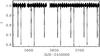 |
Fig. 1 KIC 3858884 detrended light-curve of Q8 and Q9 quarters after rebinning and normalization to the quarter median. Normalized flux is denoted with l. |
2. Kepler photometry
KIC 3858884 has been in the Kepler target list since the beginning of the mission. It has been observed both in the “short cadence” (SC) and “long cadence” (LC) mode; in these modes, the original integration times of about 6s are summed onboard and yield a final integration time of, respectively, 59s and 29.4m (Gilliland et al. 2010). Short cadence is available for a small number of targets (0.3% of the total), therefore for each run targets are inserted in or dropped from the SC observation list according to priority criteria. Also the LC mode has its priority list, and as a consequence, observations of a given target can be available for some runs only. Kepler data are delivered in “Quarters” (Q0, Q1, ..., Qn), typically three months long. (A quarter ended when the spacecraft rolled to re-align its solar panels.) KIC 3858884 was observed in the SC mode during quarters Q2, Q8 and Q9 (a total of 358307 observed points) and in the LC one during quarters Q0, Q1, Q2, Q3, Q4, Q8, Q11, Q12, Q13, and Q15 (39 949 points). Because the eclipses of KIC 3858884 last between 16 and 18 h and the dominant pulsation frequencies correspond to periods of a few hours, we used mainly the short cadence data for our analysis, which assured a dense sampling at crucial orbital phases (and a higher Nyquist frequency).
The simple aperture photometry (SAP) data from the MAST Archive1 were cleaned of obvious outliers and normalized to the median value of each quarter, by using the Pyke tools (Still & Barclay 2012). The Q2 data cover 89 days and Q8 and Q9 data 170 days for a total of about 10 orbital cycles. A section of this light curve corresponding to Q8 and Q9 quarters is shown in Fig. 1, where the data were re-binned to 600s for better visibility. The blow-up of Fig. 2 shows the pulsations and eclipses in greater detail.
Thanks to the results of L12 we already had preliminary values for the binary period and eccentricity ( and e = 0.46). Their binary model, however, is from fitting a binary-only light curve that was obtained by prewhitening the original one with all the frequencies detected in its out-of-eclipse sections. This is certainly an overcorrection, because the light curve of a system with high eccentricity, fractional radii, and orbit orientation, such as those obtained in L12, will show binary signatures out of eclipse as well. Stronger surface distortion and enhanced proximity effects at periastron are at the origin of the typical bump appearing in the light curve of eccentric systems in the shorter phase interval between eclipses. As a consequence, though restricted to the out-of eclipse sections, the harmonic analysis will still contain the orbital frequency and its overtones. These frequencies belong to the binary signal and should not be prewhitened, since they are not related to pulsation.
To estimate the relevance of this effect we used PHOEBE (Prša & Zwitter 2005) to compute a binary model with the parameters of L12. The resulting synthetic light curve (after adding Gaussian noise with standard deviation from their prewhitened binary light curve) was analyzed in the out-of-eclipse sections with PERIOD04 (Lenz & Breger 2005). The evidence was that the eccentricity bump, in that case, yields significant orbital overtones up to 15forb. Therefore, in the following, after performing the harmonic analysis with both PERIOD04 and SIGSPEC (Reegen 2004), we excluded from prewhitening the orbital frequency overtones up to the value found in the simulation.
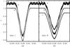 |
Fig. 3 Sections of the phased light curve around minima. Left panel: primary minimum; right panel: secondary minimum. Δφ is the phase difference with respect to conjunction phase. The curves labeled with “a” are derived by phasing LC0; curves “b” after prewhitening with pulsations, with no correction for visibility during eclipse. Curve “c” of the right panel is prewhitened taking visibility into account (see text). |
The disentangling of the EB signal from pulsations is typically performed with an iterative procedure (see, e.g., Maceroni et al. 2013, hereafter MMG13). The process consists in 1) prewhitening the original light curve (LC0) with the frequencies from the harmonic fit computed outside eclipses (if necessary after replacing the eclipse points with a local fit); 2) subtracting from LC0 the binary model obtained by fitting the residuals of the previous step; 3) prewhitening again LC0 with the harmonic fit, determined this time on the full curve; the last two steps are iterated until convergence.
This procedure was, for instance, successfully applied in the analysis of CoRoT 102918586 (MMG13), a grazing eclipsing binary with a γ Dor component whose pulsation amplitude is comparable to the (single) eclipse depth. In the case of KIC 3858884, however, a large portion of the eclipsed star is out of view during eclipse, because the orbital inclination is close to 90 degrees (88.8° in L12). As a consequence, the pulsations computed out of eclipse cannot be subtracted “as are” at all phases. This is evident from Fig. 3 showing a blow-up of both minima of the phased light curve before (curves labeled with “a”) and after (curves “b”) subtracting the pulsations, whose computation is described later in this section. The ephemeris used for phase computation of the curve is given in Eq. (1).
From inspection of the top curve of each panel of Fig. 3, we conclude that the pulsating star is the secondary component or, more precisely, that the greatest periodic luminosity variations belong to the secondary star, since the dispersion due to pulsations of the folded curve decreases significantly only during secondary minimum (Min II). The curves “b” show the effect we mentioned before: if the visibility of the pulsating star is not taken into account, the mere subtraction of the harmonic fit from out-of-eclipse sections increases the scatter around secondary minimum with respect to that of the original curve. The opposite is true for the primary minimum, since in that case the pulsating star is in full view.
In light of this evidence we modified the disentangling procedure as follows. The first harmonic analysis was performed on LC0 after replacing the eclipses with a local fit of the neighboring points and Gaussian noise. This yielded about 300 frequencies, with a significance criterion of the ratio of amplitude to local noise S/N > 4, according to the criterion proposed by Breger et al. (1993). We then subtracted the harmonic fit from LC0, excluding the orbital overtones up to 18 forb, and computed a preliminary binary model with PHOEBE, just to estimate, for each point, the fraction of light from the pulsating star at that time with respect to the median value. We assumed that the amplitude of pulsations during eclipse is also reduced by this factor, and weighted the harmonic fit to be subtracted from LC0 accordingly. This is only a rough estimate, because the actual value of this fraction certainly depends on the pulsation mode and the spherical wave-numbers, ℓ and m, (sectorial modes will act differently from tesseral or axisymmetric modes), but even this first-order treatment is sufficient for a meaningful decrease in the dispersion (see the lower curve in the right panel of Fig. 3, labeled with “c”).
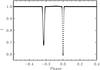 |
Fig. 4 Phased light curve of the eclipsing binary as residuals of the corrected harmonic fit, orbital overtones excluded. Phases are derived using the ephemeris of Eq. (1). |
The phased final curve due only to the orbit is shown in Fig. 4. For the sake of brevity, we show only the final outcome of the disentangling procedure (after two stages of the prewhitening of LC0). To reduce the computing time in binary modeling, the input light curve was phased and further binned with a variable step (that is, we computed normal points in phase bins of 0.0004 and 0.001 in and out of eclipse). The total number of points of the curve is then reduced to 1106. On the other hand, the harmonic analysis and prewhitening was performed at first on the full time series. When it became evident that there was no power in the Fourier decomposition at frequencies higher than 50 d-1, we binned also this time series to a time interval of 600s.
An accurate orbital period was derived by analyzing the prewhitened time series with the analysis of variance (AoV) algorithm of Schwarzenberg-Czerny (1989), as implemented in the VarTools program (Hartman et al. 2008) following Devor (2005). For this computation we also used the LC curves, which cover a longer timespan (1153d or 44 orbital cycles).
The resulting ephemeris is  (1)
(1)
3. The spectroscopic follow-up of KIC 3858884
A follow-up campaign with different instruments was necessary to get high-resolution spectra covering the long orbital cycle with a good sampling. The observations were performed with the Coudé echelle spectrograph at the 2 m telescope of the Thüringer Landessternwarte (TLS) Tautenburg (Germany), with the Bohyunsan Optical Echelle Spectrograph (BOES) at the 1.8 m telescope at Youngcheon (South Korea), with the HERMES spectrograph at the 1.2 m Mercator telescope at the Roque de los Muchachos Observatory (La Palma, Spain), and with the HRS spectrograph at the 9.2 m Hobby-Eberly telescope (HET) at the McDonald Observatory (US). The journal of observations is given in Table A.1, which also lists the measured radial velocities (RVs).
The spectral ranges and resolving power are 472−736 nm, R = 32 000 for the TLS; 380−900 nm, R = 85 000 for the HERMES; 350−1050 nm, R = 30 000 for the BOES; and 440−585 plus 610−780 nm, R = 30 000 for the HET spectra. All spectra were reduced using the following steps: cosmic ray hits removal, electronic bias subtraction, flat-fielding, electronic bias and straylight subtraction, spectrum extraction, 2D wavelength calibration, and normalization to the local continuum. Standard ESO-MIDAS packages and a special routine to calibrate the instrumental zero point in radial velocity by using a large number of telluric O2 absorption lines were used for the TLS spectra. The HERMES and HET spectra were reduced using the corresponding spectrum reduction pipelines (Raskin et al. 2011; Mack et al. 2013) and the BOES spectra using the IRAF tools.
The average signal-to-noise ratio (S/N) of the spectra from the different instrument is S/N = 160 (TLS), S/N = 120 (HET), S/N = 170 (BOES), and S/N = 44 (HERMES).
4. Spectroscopic analysis
4.1. Spectrum decomposition
For the analysis of the spectra of the components, we decomposed the observed, composite spectra using the Fourier-transform-based KOREL program (Hadrava 2004, 2005). This program optimizes the orbital elements together with the shifts applied to the single spectra of the components to build the mean decomposed spectra.
Whereas we used all the spectra for measuring the RVs, only the TLS spectra were included to derive the decomposed spectra. The reasons are that the HERMES spectra have much lower S/N (due to small exposure times), the HET spectra show badly normalized Balmer line profiles, and the BOES spectra suffer from a slight ripple in the continua that causes problems in the continua of the decomposed spectra as described below.
There are two drawbacks of the program. One comes from using the Fourier transformation. The zero frequency mode in the Fourier domain is unstable and cannot be determined from the Doppler shifts alone (Hensberge et al. 2008). This effect gives rise to low-frequency undulations in the continua of the decomposed spectra and in many cases prevents an accurate determination of the local continua. The undulations are enhanced when broad lines like Balmer lines occur in the spectral region of interest or when the input spectra already show slight undulations in their continua. The problem can be overcome when the line strengths of the stars vary with time and the degeneracy of the low frequencies in the Fourier domain is lifted.
The second problem is common to all methods of spectral disentangling, namely that the produced decomposed spectra are normalized to the common continuum of the composite input spectra. For the spectrum analysis, however, we need the spectra normalized to the continuum of the single components. Such a renormalization can only be performed when the flux ratio between the components is known. In a first attempt, we computed the expected luminosity ratio in the Strömgren b and y bands for the stellar parameters derived in the light curve solution with PHOEBE. These two passbands cover or enclose the wavelength range of our spectra. However, the decomposed spectrum of the secondary component had, after normalization, line depths greater than unity (or normalized fluxes below zero) so that we must assume that the flux ratio derived from the light curve was too small. We, therefore, included the determination of the wavelength dependent flux ratio in the spectrum analysis by using it as an additional free parameter (see Lehmann et al. 2013, for a description of the method).
For the spectral disentangling with KOREL, we used the wavelength range 472 to 576 nm, from the blue edge of the TLS spectra to the wavelength where stronger telluric lines become visible. In the solution, we fixed the orbital period to the value obtained from the LC analysis, which is much more precise than we can derive from the spectra alone. In the program setup, we allowed for variable line strengths. In a first step, we computed two solutions, the first one by including the spectra taken during primary minimum and a second one without these spectra. The comparison showed that in the first solution the decomposed spectrum of the primary was slightly broadened by the strong Rossiter-McLaughin effect (RME). The second solution, on the other hand, showed a strong undulation of the continuum of both decomposed spectra. The reason can be found in the above-mentioned lifting of the degeneracy of the low Fourier frequencies by the variable line strengths, which does not work anymore when excluding the primary eclipse from the computations. Finally, we found a compromise by excluding all but two spectra taken at Min I. The resulting decomposed spectra no longer showed any undulations, and no difference in the line profiles compared to the exclusion of all spectra around Min I could be found.
4.2. Spectrum analysis
The decomposed spectra of the components were analyzed using the spectrum synthesis method. This method compares the observed with synthetic spectra computed on a grid in atmospheric parameters and uses the χ2 of the O−C residuals as the measure of the goodness of fit (see Lehmann et al. 2011, for details). We used the SynthV program (Tsymbal 1996) to compute the synthetic spectra based on a library of atmosphere models calculated with the LLmodels code (Shulyak et al. 2004). Both programs are non-LTE based but provide the opportunity to vary the abundances of single chemical elements.
As mentioned before, we added the flux ratio as a free parameter to the analysis of the spectra. It means that the analysis had to be performed on both decomposed spectra simultaneously, searching for the best fit in the atmospheric parameters of both stars and the flux ratio between them. Free parameters of our fit are effective temperatures Teff , metal abundances [M/H], microturbulent velocities vturb, and projected equatorial velocities v sin i . Because of its ambiguity with Teff and [M/H], we fixed the log g of both components to the values obtained from the LC analysis. We started with scaled solar abundances for the [M/H] of both stars. After finding the best solution in all parameters, we normalized the decomposed spectra again according to the derived flux ratio. Then we fixed all the parameters to the derived ones and repeated the analysis for both spectra separately by varying the abundances of all chemical elements where contributions could be found in the spectra, starting with the abundance tables corresponding to the derived [M/H]. In a next step, after optimizing all individual abundances, we repeated the analysis of both spectra as described above based on the modified abundance tables. Changes in the atmospheric parameter values have been marginal so that we stopped at this point.
Table 1 lists the results of abundance analysis, and Table 2 gives the final atmospheric parameter values. The second column of Table 1 gives the atomic number, and the third the assumed solar abundance as log (Nel/Ntotal), corresponding to Asplund et al. (2005). The fourth and fifth columns list the difference with respect to the solar value (+ means enhanced). The parameter errors represent 1σ errors. The atmospheric parameters were derived from the full grid of parameters but for both components separately. The ambiguity among the parameters is included in the error analysis in this way per star. We did not have enough computer power to include the combined effects from both stars in the error calculation. These effects arise during the combined analysis necessary to determine the flux ratio, e.g., because of the influence of Teff,1 on the parameter values of the secondary component. For the abundances, we included the Teff of the corresponding star in the error analysis of the single elements.
Abundances of the binary components.
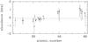 |
Fig. 5 Abundances of the primary (asterisks) and secondary (open circles) components in dex relative to the solar values. The dashed and dotted lines mark the [Fe/H] of the primary and secondary components, respectively. |
Figure 5 shows the abundances sorted by their atomic number. The derived abundances of both components agree within their 1σ errors for all but three elements. The outliers are Fe and Ni, the elements with the smallest abundance errors, and Sc. In the case of Fe and Ni, this could be a hint that the errors were underestimated. In the case of Sc, on the other hand, the difference of 1.23 dex can be confirmed from a visual inspection of the decomposed, as well as of the observed, composite spectra.
Because of the ambiguity between Teff and abundances, it is important to note that the abundances given in Table 1 are based on the spectroscopically derived Teff. They are part of a consistent spectroscopic solution, but may vary if a different Teff (such as the value derived from the combined light and radial velocity curve solution, see Sect. 5) is assumed.
The distribution of the abundances with atomic numbers of the primary component resembles that of BD +18 4914 which is said in Hareter et al. (2011) to be an Am star. These are chemically peculiar, early F to A stars. They are characterized by slow rotation (cut-off of about 100 km s-1 ), underabundance of C, N, O, Ca, and Sc, and overabundance of the iron peak and rare earth elements (see, e.g., Iliev & Budaj 2008, for an overview). Our two stars show rotation that is not too fast and an overabundance of the heavy elements but not of those of the iron peak. Only one of the stars, the non-pulsating primary component, shows a significant underabundance of Sc.
Atmospheric parameters of the binary components.
5. Light and radial velocity curve analysis
The light and radial velocity curve solutions were performed with the current (“stable”) version of PHOEBE. We preferred a non-simultaneous solution of light and radial velocity curves, since the RV data are acquired at different epochs with respect to photometry, and the two data sets are very different in terms of observed point number and accuracy. On the other hand the two solutions were connected by keeping fixed in each of them the parameters that are better determined by the other type of data.
Orbital parameters derived with KOREL (K) and from the cleaned KOREL (K + P) and TODCOR (T + P) RVs using PHOEBE.
5.1. Radial velocities and preliminary orbital solution
We used two different programs, KOREL and TODCOR (Mazeh & Zucker 1994; Zucker & Mazeh 1994), to measure the radial velocities (RVs) and PHOEBE to derive the orbital parameters. This allowed to cross check the results but also to profit from the advantages of each method: KOREL provides disentangled spectra and performs better in the analysis of spectra at conjunction phases, while TODCOR is simpler and yields a more straightforward and consistent determination of uncertainties. In both cases the included spectral range was 472−567 nm, which does not contain broad Balmer lines and is almost free of telluric lines. KOREL delivers the velocity shifts with respect to the composite spectrum and, directly, the searched orbital parameters. As first step we obtained a preliminary orbital solution, based on all the out-of-eclipse spectra, which is given in column K of Table 3. In the following, we used all spectra, including those at eclipse phases. Since KOREL does not provide straightforward error estimates on the derived parameters (nor on the RV shifts) and does not consider the RME and proximity effects, a fit of the KOREL RV curves was performed with PHOEBE, in order to independently obtain the orbital parameters together with their errors.
PHOEBE calculates the orbit by simultaneously fitting the RV curves of both components and includes the RME, though only in the hypothesis of alignement of rotation and orbit axes, and the proximity effects (on the basis of a model of the surface brightness distribution from the light curve fit). The adjusted parameters were the system semi-axis a, the eccentricity e, the longitude of periastron ω, the mass ratio q, the barycentric velocity γ, and the origin of time in PHOEBE, from which we derived the epoch of periastron passage, T. Figure 6 shows the KOREL shifts and the PHOEBE best fit.
We subtracted the resulting fit from the observed RVs and performed a period search in the residuals with PERIOD04. For the secondary component, we found the same two frequencies that dominate the oscillations in the Kepler light curve (see Tables 4 and B.1). No periodic short-term variations were instead found for the primary. Finally, we obtained the final fit with PHOEBE, after prewhitening the secondary RV curve with the detected frequencies. The results are listed in Table 3 in column K + P. The listed uncertainties are the formal errors of the fit and are certainly underestimated, because of having the same origin (see Sect. 5.4) and of the lack of errors of the KOREL RVs.
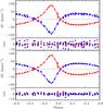 |
Fig. 6 Upper two panels: phased RV shifts of KIC 3858884 components from KOREL. Filled circles: primary star. Filled squares: secondary star. Curves: PHOEBE fit. Second panel: fit residuals, with the same symbols. Lower two panels: the same after prewhitening with the two significant frequencies found in the residuals. |
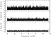 |
Fig. 7 Amplitude spectra, based on our complete dataset of 83 spectra. From top to bottom: original data, largest peak f1; f1 subtracted, largest peak f2; f1 and f2 subtracted. |
Frequencies found in the residuals of the RV fit of the secondary component, based on the RVs derived with KOREL and with TODCOR.
Because the described procedure is a mixture of two different methods – the RVs are determined in a procedure that does not account for the RME and proximity effects, whereas the calculation of the orbit with PHOEBE includes them – and because of the problems in getting a sound estimate of the errors, we redetermined the RVs from the observed spectra by using the implementation of the TODCOR algorithm by one of the authors (HL).
TODCOR is applied to the observed composite spectra and performs a 2D cross-correlation for the contributions from each star, using two different templates. We used two synthetic spectra as templates based on the parameters obtained for the two stars from spectrum analysis (see Sect. 4). The resulting RVs of both components are listed in Table A.1 of the Appendix. Also in this case, we computed the spectroscopic orbit with PHOEBE and performed the analysis of the residuals with PERIOD04 to find the same two frequencies as from the KOREL RVs (Table 4), and derived the final fit after prewhitening them. Figure 7 shows the finding periodograms. The final orbital parameters are listed in column T + P of Table 3.
The comparison of the results obtained from the KOREL and the TODCOR RVs shows that they have about the same accuracy. All orbital parameters agree within 1σ. Moreover, all the derived frequencies of the short-term variations are in perfect agreement and agree with the photometric ones. Taking both parameter sets together, we can say that the most important parameter, the mass ratio, is q = 0.993 ± 0.012. This is a conservative estimation that assumes that the two methods are of comparable accuracy.
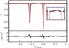 |
Fig. 8 Upper panel: phased light curve of the eclipsing binary and the final fit with PHOEBE (full line, in red in the online version), inset: a blow-up around periastron phase showing the fit around periastron phases. Lower panel: fit residuals. |
In Fig. 6 we preferred to show the RV shifts from KOREL, because that method provides a few more points around primary minimum, allowing the Rossiter-McLaughin effect to be better traced. For the combined photometric/spectroscopic solution, however, we will favour the TODCOR-based result as input. The reason is that its derivation seems to be more consistent, keeping in mind that the KOREL solution is based on RVs derived without considering the Rossiter-McLaughin and proximity effects, which were computed with PHOEBE to get the errors of the parameters.
The inspection of the radial velocity curves confirms that the dominant pulsations belong to the secondary component, since the RME, visible in both curves, indicates that the component showing pulsation-related scatter in velocity is the one eclipsed at phase ~0.77 (or − 0.23). On the other hand neither from the light curve nor from spectra can we deduce that all the components of the periodical pattern detected in the light curve belong to the same star.
The in-eclipse RV points are too few for modeling RME and deducing information on the rotation axis alignment. The apparent symmetry around the unperturbed curve of the four points at primary minimum are consistent with a parallel rotation axis of the primary component.
5.2. Light curve solution
In the light curve solution we adjusted the inclination i, the secondary effective temperature Teff,2, and the surface potentials Ω1,2. The primary passband luminosity L1 was separately computed rather than adjusted, since this allows for a smoother convergence to the minimum. The mass ratio q was instead fixed to the values derived from the fit of the radial velocity curves (from TODCOR parameter set); the eccentricity e, and the longitude of periastron ω, were initially fixed to the spectroscopic values and only finely tuned in the light curve fit.
For limb darkening we adopted a square root law that employs two coefficients, xLD and yLD, per star and per passband. The standard Kepler transmission function in PHOEBE is the mean over the 84 different channels of the Kepler FoV. PHOEBE determines the coefficients by interpolating, for the given atmospheric parameters, its internal look-up tables. The gravity darkening and albedo coefficients were kept fixed at their theoretical values, g = 1.0 and A = 1.0 for radiative envelopes (von Zeipel 1924).
The primary effective temperature was kept fixed, since it is well known that the solution of a single light curve is only sensitive to relative values of the effective temperatures. We used the value Teff,1 = 6800 K, which was provided by the analysis of the spectra. The uncertainties on the effective temperatures are essentially those from spectra analysis, since the additional term on Teff,2 from the fit is very small (a few degrees). A shift in Teff,1 is reflected in a shift of Teff,2 in the same direction, leaving the ratio almost constant.
Figure 8 shows the fit and its residuals. The larger scatter of residuals around minima depends on the smaller phase bins used for the eclipses. The remaining features around minima are instead related to the stellar surface representation in PHOEBE (and WD), in which the aligned border of the first tile of each meridian produces a seam along the central line facing the companion (y = 0, in the corotating frame centered on the star). This issue will be solved in the next PHOEBE version, still under development2.
5.3. Combined solution
The system parameters from the light and radial velocity curve solution are collected in Table 5. The system model corresponding to the best fit is formed by two similar stars: masses differ by 0.02 M⊙, radii by 0.42 R⊙, and effective temperatures by less than 200 K.
Orbital and physical parameters of KIC 3858884.
There is an evident discrepancy between our combined solution and the results from the analysis of the disentangled spectra. According to Table 2, the hottest star (by ~70 K) is the secondary component. On the other hand we do know, as mentioned in the previous section, that the secondary, pulsating star is eclipsed at the widest and least deep minimum. The shape of the light curve cannot be reproduced by a hotter secondary. Even considering the effect on the eclipse depth of the different distance between the stars at minima because of eccentricity, stars with the same temperature yield a secondary eclipse that is not as deep (only a few percent), and the difference in depth will still decrease (and then change sign) for a hotter secondary, while the observed value amounts to about 10%. A cooler secondary is, therefore, needed to reproduce the light curve shape. Considering that the line profiles of the secondary star are certainly affected by pulsations, we decided to trust, and adopt in the following, the Teff,2 value from the light curve modeling. The uniqueness of the solution and the derivation of parameter uncertainties are discussed in the next section.
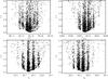 |
Fig. 9 Blow up of the PIKAIA results: cost function value vs. inclination (top left), secondary temperature (top right), and potentials (bottom panels). The minimum value is indicated by a gray (red in the electronic version) larger dot. |
5.4. Uniqueness of the solution and parameter uncertainties
The light curve fit is obtained by minimizing a cost function that measures the deviation between model and observations in the space of adjusted parameters. In PHOEBE the minimization is done by differential correction, in the Levenberg-Marquart’s variant or by the Nelder and Mead’s downhill simplex. As a consequence, it suffers from the well known problems of these methods: the minimization algorithm can be trapped in a local minimum or degeneracy among parameters, and data noise can transform the minimum into a large and flat bottomed region, or an elongated flat valley, rather than a single point. Besides this, the correlation among the parameters implies uncertainties on the derived values that are significantly larger than the formal errors derived, for instance, by the least square minimization. The disagreement between the analysis of photometry and spectroscopy was an additional reason to test the uniqueness of our photometric solution.
The search for the global minimum can be performed with a variety of techniques, which have in common, however, a large demand in terms of computing time. Prša & Zwitter (2005), for instance, propose heuristic scanning and parameter kicking (a simplified version of simulated annealing). The former method was applied to solve the CoRoT light curve of the eccentric binary HD 174884 (Maceroni et al. 2009).
Another popular choice is that of genetic algorithms, a class of optimization techniques inspired from biological evolution through natural selection of the fittest offsprings. A widely used implementation of genetic algorithms in astrophysical problems is PIKAIA3 (Charbonneau 1995). Its input is a randomly chosen population, whose individuals are characterized by the values of the parameters to optimize (the values are coded in their “chromosomes”). Pairs of individuals are mixed through a breeding process that yields “offsprings”, the members of the new “generation” are chosen on the base of their fitness, measured by a user-defined cost function. Random mutation of some of the offsprings is also included. Thanks to the weighting of offsprings with fitness and to the mechanism of breeding (which allows information to be incorporated from the previous generation), the search process of PIKAIA is much faster than in random-search algorithms (e.g., Monte Carlo).
We built an interface program FITBINARY, which connects PIKAIA (v1.2) to the PHOEBE’s underlying fortran code (a PHOEBE specific version of the Wilson & Devinney (1971) code). We preferred to stick to the PHOEBE back-end WD-version because of its many extensions and of its internal computations of outgoing fluxes and limb darkening in the Kepler bandpass. In this way, the FITBINARY results are fully compatible with PHOEBE modeling.
The PIKAIA search was performed on the same parameters adjusted in PHOEBE: inclination, surface potentials, and the effective temperature of the secondary component, while the primary passband luminosity was recomputed at each step. We made use of the creep mutation mode to jump over the so-called Hamming walls (see the online PIKAIA documentation). The search was first conducted in a large region around a provisional set of parameters, to later on be restricted to smaller intervals. A typical scan (100 generation of 50 individuals) requires about 40 h of computation on a 1.8 GHz Intel Core i7 processor with 4Gb RAM. For a non-eccentric system the computation is much faster, since it is not necessary to recompute the surface geometry at each orbital phase.
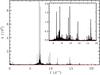 |
Fig. 10 Final amplitude spectrum of KIC 3858884 and, in the inset a blow-up of the same spectrum after prewhitening the two highest frequencies. The gray line (red in the online version) is the significance threshold, which is four times the local noise (computed on the residual spectrum with a box of 3 d-1). |
Figure 9 displays the results of the genetic algorithm, the four panels display the cost function (in arbitrary units) versus the four parameters. The clustering of points along vertical strips indicates the efficiency of the method in converging to the minimum. The figure is actually a blow-up around the minimum, since the search was performed in wider parameter ranges than those displayed (i = 88.1−88.3, Ω1 = 18−19, Ω2 = 20−21, Teff,2 = 6550−6650). When looking for instance at the Ω2 plot, it is evident, that a “blind” minimum search could be trapped in any of the parabolic regions. The parameters of Table 5 are derived from the parameters of PIKAIA’s minimum.
The uncertainties on the final parameters and the corresponding one-sigma errors of Table 5, were computed with bootstrap resampling (BR) both for the radial velocity and the light curve fit, according to the scheme described in detail in Maceroni & Rucinski (1997) and Maceroni et al. (2009) and applied in MMG13. The main difference with the standard BR treatment is that the procedure is performed within the minimum already established by a single iterated solution (that is, using only one set of residuals and parameter derivatives computed in the global minimum). This is because the full computation of an iterated minimization for each bootstrap sample (we used 20 000 samples) is extremely heavy in terms of computing time, especially in the case of an eccentric orbit, which requires recomputation of the binary surfaces at each phase. The Markov chain Monte Carlo (MCMC) used in other cases (da Silva et al. 2013) is too demanding in terms of computing time in the case of an eccentric system.
6. Pulsational properties
6.1. Frequency extraction
The frequency spectrum of the residual light curve, after subtraction of the final binary model, is shown in Fig. 10. The plot is restricted to the frequency interval containing meaningful features. Since the residuals of Fig. 8 are dominated by deviations around minima, we computed the frequency spectra both for the full residuals and for the out-of-eclipse sections. The spectra are very similar. The main difference is the presence, in the first case, around the two dominant frequencies of a large number of low-amplitude peaks that are spaced by multiples of the orbital frequency. The spurious nature of these features is proven by comparison with the out-of-eclipse Fourier spectrum, in which they disappear. For this reason we adopt and discuss the results obtained from the light curve cleaned of the EB signal in the following but exclude the eclipse sections.
As in our preliminary analysis, we used both SIGSPEC and PERIOD04 for frequency extraction. SIGSPEC has the advantage of automatically computing the frequency components and their spectral significance ξ, which is related to the false alarm probability of detecting a feature actually due to (white) noise as a peak: ξ = −log (ΦFA) (Reegen 2004). PERIOD04 was used to check the results, to compute the local noise spectrum, and to derive the S/N.
A commonly adopted frequency significance threshold is the one suggested by Breger et al. (1993), i.e. a S/N value of the amplitude ≥4. This value, however, was actually derived for ground-based multisite campaigns and is also based on the assumption of random noise. This may not be the case for Kepler data or pulsating stars, which can show significant red noise (Kallinger & Matthews 2010). According to Reegen (2007), the approximate correspondence between spectral significance and S/N yields ξ(S/N = 4) = 5.47. We checked, however, that in our dataset we should not go below ξ ≃ 12 to have a S/N > 4 everywhere (and, in particular, at low frequencies). We therefore adopted this more conservative criterion for significance.
Table B.1 lists the first sixty out of about four hundred frequencies in order of detection and their spectral significance, and the full table is available at the CDS. The uncertainties in the table were computed according to Kallinger et al. (2008) and are noticeably larger than the formal errors of the LS fit. The obvious combinations of frequencies and the overtones of the orbital frequency (forb = 0.0385327) are also listed in the comments.
The inspection of Fig. 10 and Table B.1 reveals that pulsations occur with frequencies in two separate regions of the spectrum: a high-frequency region above 6 d-1, containing most of the signal, and a low-frequency one (around or below 1 d-1), whose strongest frequency, f13 of the table, has an amplitude ~4% of f1. The first region is where one expects p-mode pulsations for classical δ Sct stars, the second is the typical region of g-modes in γ Dor stars.
As our pulsator is a highly eccentric binary one can also expect that the orbital motion and the varying tidal forces along the orbit affect the pulsations. According to Shibahashi & Kurtz (2012), the Doppler effect from orbital motion in a pulsating binary component causes a phase modulation of pulsation. That yields, in the Fourier decomposition of the time series, a multiplet with the original frequencies split in components separated by the orbital frequency. The amplitude of the multiplet components depends on the binary parameters and on the ratio of the orbital and pulsation periods. Using the relations of the above-mentioned paper, we derived the ratio of the amplitude of the first multiplet components (± iforb;i = 1,2) to the central frequency for the case of an eccentric binary. (Symmetric ±peaks have the same amplitude.) We find that the amplitude of this first component should be ~1.5% of the central frequency, while that of the second 0.3%; the latter is too a low value for our detection threshold, even for the strongest frequencies. In our frequency list we find at least the first component (i = 1) of the multiplets around f1,2, with an amplitude somewhat higher than expected, but at least of the right order (f4,f19,f45, of Table B.1, while f81 = f2 − forb can be found in the complete version at the CDS).
We could not find, instead, in the Fourier spectrum the signature of stellar rotation (which corresponds to a rotation frequency frot,2 = 0.167 d-1, according to the measured v sin i and the derived values of inclination and stellar radius). The ratio between the rotation and break-up velocities is low enough (vrot,2/vb,2 ~ 0.008) to expect equidistant multiplets (Reese et al. 2006). These should be easy to spot, but the high number of frequencies and the uncertainty on the rotation velocity prevent detection.
6.2. High-frequency variability
An estimate of the pulsation frequency regime for a δ Sct can be derived by the relation between the frequency of a radial mode and the mean density through the pulsation constant Q (Stellingwerf 1979): 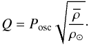 (2)Typical Q values in the δ Sct domain are Q = 0.033 for the fundamental radial mode and decrease to 0.017 for the third overtone. For single stars, the mean density is inferred from Teff, the absolute magnitude, and surface gravity, but in our case we have an accurate determination of mass and radius from the binary model. The pulsation frequencies corresponding to the fundamental and the first three overtones for the secondary star, with the mentioned Q values, are in the range 7.8−15 d-1. For the primary star the interval is from 6.5 to 12.5 d-1. That corresponds to the frequency interval where we find most of the signal. A more precise computation of the excited frequency ranges, based on theoretical models, is presented in Sect. 7.
As Breger et al. (2009) point out, the numerous observed frequencies of δ Sct often appear in groups that cluster around the frequencies of radial modes and show some regularity in spacing. This is put in relation to mode trapping in the envelope, which increases the probability of detection (Dziembowski & Królikowska 1990). These modes are the non-radial counterparts of the acoustic radial modes and, for low ℓ degree, have frequencies close to those of radial modes. In the case of δ Sct pulsators, theory predicts a much higher efficiency of mode trapping for ℓ = 1 modes, as in Breger et al. (2009).
These authors introduce a theoretical diagram that displays the average separation of the radial frequencies versus the frequency of the lowest frequency unstable radial mode (their Fig. 8, s − f diagram). The values are arranged on a grid with the different radial modes and surface gravity as parameters. The location of a pulsator in that diagram allows, therefore, the estimation of its surface gravity (if the radial mode is assumed or known). The histogram of the frequency difference is shown in Fig. 11 both for the whole set of frequencies and for those with an amplitude A > 10-4 (~100 frequencies). There is an evident pattern, indicating a separation of the radial modes of s ≃ 2.3 d-1. One sees, in fact, a first peak at 2.3 d-1and others at approximately two and three times the value. (The separation of radial modes is not exactly constant with increasing order.) Since we already have a precise estimate of the gravities, we used the value of s to derive the frequency of the fundamental radial mode of the secondary, which is ~7.4 d-1, i.e. very close to the values of f2. We know that both f1 and f2 belong to the secondary component, if – as is plausible – we assume that f2 is its fundamental radial mode, f1 should be a non-radial one. The lower frequencies in the same domain could be either non-radial modes of the secondary or radial/non-radial modes of the primary component.
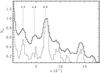 |
Fig. 11 Distribution of differences among the detected frequencies (every frequency was subtracted from all the others and the plot is restricted to the positive values). For easier comparison, each histogram is normalized to the local maximum around 7 d-1. The black line refers to the whole set of 403 frequencies, the gray line to those with amplitude larger than 10-4. The histograms show that there is a preferred spacing around 2.3 d-1, which is clearly visible in both distributions. According to Breger et al. (2009), the spacing corresponds to spacing between radial modes. The multiples of the spacing are also indicated by dotted lines. |
6.3. Low-frequency variability
The low frequencies detected in the range of high-order g-modes, typical of the γ Dor variables, could indicate the hybrid nature of the δ Sct pulsator. According to the asymptotic approximation (Tassoul 1980), the angular frequency, σnℓ, of high-order g-modes of radial order n and angular degree ℓ propagating between two convective regions is given by 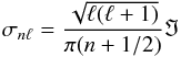 (3)where
  dr is the integral of the Brunt-Väisälä frequency (N), weighted by the radius, along the propagation cavity.
For the stellar structure and frequencies of interest here, r1 and r2, hence ℑ, weakly depend on the mode. As a consequence, the first-order asymptotic approximation also predicts that high-order g-modes should be regularly spaced in period, with a mean period spacing: 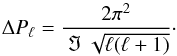 (4)Moya et al. (2005, hereafter M05) derive from Eq. (3) a straightforward relation between radial orders, frequencies, and corresponding ℑ values, for modes with the same ℓ value:
  (5)The second approximation is justified by the weak dependence of ℑ on the order, for the modes of interest here. We verified whether such a relation holds among the frequencies in the interval 0.3−3.0 d-1. We computed the expected n ratios for radial orders 1 < n < 120, in the hypothesis of the same degree ℓ, and compared the results with the observed ratios of the four locally highest amplitude frequencies (f13, f41, f47, f55, see Fig. 12), excluding from the search the obvious combinations, such as f61 = 0.4930 d-1= f4 − f1. We assumed a tolerance for each ratio of 0.004 d-1, which takes both the deviations of the asymptotic relation with respect to the theoretical models, see M05, and the uncertainties on the derived frequencies into account. We found, indeed, a few combinations of radial orders reproducing, within the uncertainties, all the observed ratios (Table 6).
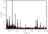 |
Fig. 12 Frequency spectrum in the γ Dor domain after prewhitening with the first twelve frequencies of Table B.1. The highest amplitude peak corresponds to f13 ≃ 18forb. The gray (red) line is the estimate of local noise by PERIOD04 (with a box of 0.2 d-1). The black dots denote the values used to derive the period spacing. The open circle denotes the frequency f193 = 1.2350 d-1, which according to that period spacing value has nf193 = 39. This last frequency is also very close to 32forb. |
Each combination allows the mean value of ℑ to be estimated from Eq. (3), if a value of ℓ is assumed. This yields a quantity which can be readily compared with theoretical models. Cancellation due to surface integration of the observed flux suggests low ℓ values, and, in our case, a clue to infer the ℓ value is offered by the highest amplitude frequency among the four selected being very close to an overtone of the orbital frequency, f13 ≃ 18forb. Since tidal action is more efficient in exciting ℓ = 2 modes (e.g., Kosovichev & Severnyj 1983), ℓ = 2 is the straightforward assumption. Table 6 lists the values of the integral of the Brunt-Väisälä frequency, ℑ, and of its inverse in seconds derived under this hypothesis. The comparison with the theoretical models is presented in the next section. The lines in boldface highlight the combinations in better agreement with the results of that section. The mean period spacing (and its standard deviation) corresponding to the two n series highlighted in Table 6 (and ℓ = 2) is the same: ΔP = 1736s ± 19s.
The maximum number of frequencies whose ratios follow the relation in Eq. (5) is Nm = 4. We tested that by adding to the quadruplet, the other clearly detected frequency in the interval f = 0.5 − 2.5 d-1, and within the tolerance given above, we found no consistent solution. On the other hand, by adopting the derived period spacing, we found a few frequencies that are close to the expected values for some n, for example f193 = 1.2350 d-1 (nf193 = 39), which is also close to an overtone of the orbital period (32forb). However, given the increasing uncertainties on lower amplitude frequencies and the intrinsic uncertainties in the procedure using asymptotic relations, we prefer to restrict our analysis to the firmly established quadruplet.
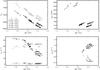 |
Fig. 13 Properties of the stellar models selected as explained in the text. In all panels different quantities are plotted as function of the model age, the symbol shape depends on the chemical composition, the grey symbols correspond to the primary star, the black ones to the secondary. Top left panel: Teff for both stars; top-right panel: the integral of the Brunt-Väisälä frequency for the secondary component; bottom left panel: the minimum and maximum excited frequency in the δ Sct domain for both stars (empty and full symbols denote, respectively, the minimum and maximum values); bottom right panel: the minimum and maximum excited frequency in the γ Dor domain for the secondary. |
7. Physical properties of KIC 3858884
Further information on the physical properties of the system can be derived by comparison with theoretical models. As in previous studies (Maceroni et al. 2013), we use the evolution of the stellar radii with time, combined with the constraint of coevality, to infer the system age. The stellar radius evolution instead of, for instance, the position in the H-R diagram, is preferred because the radii are directly and precisely determined from the radial velocity and light curve solutions, while the computation of temperature and luminosity implies the use of color transformations and bolometric corrections.
The evolutionary tracks were obtained from stellar evolution modeling with the code CLES (Code Liégeois d’Évolution Stellaire, Scuflaire et al. 2008) with the following micro-physics: equation of state from OPAL (OPAL05, Rogers & Nayfonov 2002); opacity tables for two different solar mixtures (Grevesse & Noels 1993; Asplund et al. 2005, GN93, and AGS05), from OPAL as well (Iglesias & Rogers 1996). These were extended to low temperatures with the Ferguson et al. (2005) opacity values. The nuclear reaction rates are from the NACRE compilation (Angulo 1999), except for  , updated by Formicola et al. (2004).
Convection is treated by the mixing length theory (Böhm-Vitense 1958), with the value of αMLT fixed to 1.8. At any rate, in the temperature range of interest here, its value does not affect the stellar radius. Models with and without overshooting were computed with the extra-mixing length expressed in terms of the local pressure scale height (Hp), as αOV, and αOV values equal to 0.15 and 0.20.
We computed evolutionary models for masses between 1.82 and 1.91 M⊙, with a step of 0.005 M⊙. For the chemical composition we assumed different values of the metal mass fraction (Z), from 0.007 to 0.018, and two values of the helium mass fraction Y = 0.27, and 0.28. Because of the abundance anomalies, the value of Z is not well constrained. As mentioned in Sect. 4.2, the primary shows some features of Am-Fm stars, except for the Fe overabundance. The Am-Fm phenomenon disappears or decreases with surface gravity (Kunzli & North 1998). Therefore, the slightly evolved status of the primary (log g = 3.6) could explain the particular chemical pattern. It is widely accepted that the Am-Fm phenomenon is the consequence of microscopic diffusion and radiative acceleration, together with macroscopic processes, such as rotational induced mixing or stellar wind. Radiative accelerations are not implemented in CLES, so we cannot fit the chemical pattern at the surface. On the other hand, if photospheric abundances are the results of selective diffusion processes, we have no information on the chemical composition of the whole star. Because of the above-mentioned anomalies, the Fe abundance cannot be used as a proxy for [M/H] to be used in stellar modeling.
To derive the age of the system, we selected the models such that the primary and secondary have the corresponding masses and radii at the same age and have a difference of effective temperature of ~200 K, as suggested from the light curve solution. Given the similar mass of the two components, it is possible to fit the difference in radii only if the two stars are in a different evolutionary stage, and we could get this result only if overshooting is included in the computations. We then considered solutions in which both stars have the same extra-mixing in the central regions (αOV = 0.15,0.20) and also the possibility of a different efficiency of the central mixing process in either component, by using αOV = 0.20 for the primary and αOV = 0.15 for the secondary, and vice versa.
In the following we present and discuss the models relative to the AGS05 solar mixture, which provide similar results to those with GN93 and was used as reference in Table 1. The constraint on the effective temperature of the components rules out models with the lower metallicity values. The best match is obtained for Z = 0.016 and 0.018 which means [M/H] + 0.1 or +0.15 depending on whether we assume AGS09 (Asplund et al. 2009) or AGS05, respectively. If, in addition, we fix the primary temperature to 6810 ± 140 (i.e. ± 2σ), as obtained from spectroscopy, we can discard all models with αOV = 0.15 in both stars and almost all those with different αOV in the two components (with the exception of three models with αOV,1 = 0.15 and αOV,2 = 0.20). The rejected models, in fact, reproduce the temperature difference but provide too high a value for Teff,1.
The constraints listed above select a sample of 59 stellar models with equal αOV and different chemical abundances. We dropped the three more models with different αOV after checking that the results do not change. The system age of the whole sample varies from 1.17 to 1.49 Gy (see the top left panel of Fig. 13). This interval is reduced to 1.38–1.49 Gy for the primary temperature range in Table 5. The other panels of the figure show the value of ℑ and the maximum and minimum excited frequencies in the δ Sct and γ Dor domains, as computed with the non-adiabatic pulsation code MAD by Dupret et al. (2003). From inspection of these panels we can conclude that the derived age range corresponds to
-
a value of the Brunt-Väisälä for the secondary component between 730 and 760 μHz (top right panel), while the same quantity for the primary is ~1100 μHz,
a minimum and a maximum value of the excited frequencies, in the δ Sct domain, of 5–17 d-1 for the secondary and of 5−22 d-1 for the primary (bottom left panel),
a minimum and a maximum value of the excited frequencies, in the γ Dor domain, of 0.4–1.1 d-1 (bottom right panel), the plot is for the secondary only because the excitation mechanism is not at work in the primary.
All these values are quite consistent with what was obtained in the previous section. Both stars can pulsate in the δ Sct domain (but our computations do not provide the amplitude of the frequency components so we cannot tell which one is actually detectable), while the driving mechanisms for γ Dor pulsations can only work in the secondary, which could therefore be a genuine δ Sct/γ Dor hybrid pulsator. On the other hand, our computations do not take the presence of an “external” excitation mechanisms, such as is the varying tidal force in an elliptic orbit, into account. The presence of an orbital frequency overtone among the frequencies detected in the γ Dor domain could be a clue to such an origin. To distinguish between the two hypotheses, we computed from Eq. (3) the frequencies corresponding to ℓ = 1 modes and to the selected ℑ values. The underlying idea was that, at variance with tidal forces, an intrinsic excitation mechanism would also work for ℓ = 1 modes. We found that for ℑ = 729.8 μHz, three of the detected frequencies (f68 = 0.3573, f100 = 0.3284, and f279 = 0.4686 d-1) correspond, within their errors, to expected ℓ = 1 values. Since, however, the theoretically expected g-mode frequencies are closer and closer for decreasing frequency values, an occurrence due to pure coincidence is also possible.
In Fig. 14 we show a representative pair of evolutionary tracks from the selected sample (the one in best agreement with all the constraints). It should be noticed that the fundamental radial mode of the secondary model is, in this case, f ≃ 7.5 d-1, i.e. in excellent agreement with the finding from frequency differences of the previous section.
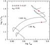 |
Fig. 14 Example of evolutionary tracks for a pair of stellar models fulfilling the constraints explained in the text, and with Y = 0.27, Z = 0.016 and αOV = 0.2. For this particular pair Teff,1 = 6860 K and Teff,2 = 6680 K, the requested difference in radius with similar masses is fulfilled thanks to a more evolved stage of the primary component. |
8. Discussion and conclusions
Thanks to the unprecedented quality of the Kepler data and to a long spectroscopic follow-up involving several different instruments, we have been able to achieve a comprehensive description of this challenging binary. As frequently happens, the availability of higher quality data is at the same time a source of achievements but also of new challenges.
The Kepler light curve has been intractable with the method currently used to analyze pulsating star in binaries (e.g., MMG13 Debosscher et al. 2013), given the high eccentricity and the deep eclipses, hence the modified oscillatory pattern during the deep eclipse of the pulsator. To face this problem we developed a new procedure for extracting the orbital (i.e., binary only) contribution to the light curve, which takes the effect of eccentricity and (at least at first order) of the eclipse of the pulsating star into account. The straightforward development would be a detailed analysis of the eclipse of the pulsator with the eclipse-mapping technique (Bíró & Nuspl 2011), which would also allow the information on the observed modes to be extracted.
The partial disagreement between the parameters derived from photometry and spectra analysis was a motivation for an extended scan of the parameter space of the light/RV curve fits, to rule out the possibility of a wrong solution corresponding to a secondary minimum. To this purpose a genetic minimization algorithm was implemented in combination with PHOEBE.
The final model of KIC 3858884 depicts a binary with components of similar mass and temperature but different radii, indicating a slightly evolved status of the more massive star. This can be the reason for the difference in the surface abundance of some elements (different efficiency of diffusion and radiative forces) and in pulsational properties. The agreement with theoretical models required including overshooting in the calculations, and the adopted value of αOV = 0.2 agrees with the results of Claret (2007) for the mass domain considered here. It has to be noticed that the masses of our components are at the lower limit of the Claret sample (whose stars all have masses above 2 M⊙, with the only exception the secondary of YZ Cas).
Both the light curve analysis, from the dispersion of the phased light curve, and the analysis of the radial velocity curves, again from dispersion and from the RME, indicate that the two dominant frequencies belong to the secondary star. These second and first highest amplitude frequencies are identified as the fundamental radial mode and a non-radial mode. The most consistent scenario from the comparison of pulsational analysis with the theoretical modeling indicates as well that the secondary component is at the origin of the high-order g-modes in the γ Dor frequency domain, as the driving mechanism is at work only in this component. On the other hand, this conclusion only applies in the hypothesis of an intrinsic excitation mechanism and the alternative explanation of tidal origin cannot be excluded.
Further insight into this interesting system could be gained by definite identification of the pulsation modes, which would increase our knowledge of the internal structure of the pulsator. That could be achieved by acquiring multicolor photometry and/or high-S/N high-resolution spectra. We think that additional spectroscopy is the best choice. The target is bright enough and the pulsation frequencies not too high to obtain, even with medium class telescopes (2−4 m), high-S/N spectra of high-resolution both in time and wavelength. Spectroscopic mode identification allows reaching higher ℓ values with respect to multiwavelength photometry, which is limited by cancellation effects. Moreover, spectra of higher S/N than obtained with the standard follow-up of Kepler targets, will more reliably determine the atmospheric parameters and hopefully solve the discrepancy of the secondary star temperature and abundances.
Online material
Appendix A: Measured radial velocities
Radial velocities (in km s-1) of KIC 3858884. The columns are BJD 2 455 000+ of mid-exposure time, instrument, RV of the primary, RV of the secondary, and RV of the secondary component cleaned for the short-term variations.
Appendix B: Frequencies in the amplitude spectrum of KIC 3858884 from the residuals without eclipses
First 60 frequencies detected in the amplitude spectrum of KIC 3858884 (from the residuals without eclipses).
The code and related documentation are freely available from http://www.hao.ucar.edu/modeling/pikaia/pikaia.php
Acknowledgments
We thank Conny Aerts for enlightening discussions and critically reading the manuscript, and Daniel Reese, Avi Shporer, Orlagh Creevey, Kevin Stassun for useful suggestions. We also express our gratitude to Andrej Prša for making PHOEBE publicly available, and for his constant support; to Paul Charbonneau, author of PIKAIA; and to Marc Antoine Dupret for making his computer code MAD available to us. We also thank the unknown referee for constructive criticisms. This work is partly based on data from the Kepler mission, which is funded by the NASA Science Mission directorate. The photometric data were obtained from the Mikulski Archive for Space Telescopes (MAST). STScI is operated by the Association of Universities for Research in Astronomy, Inc., under NASA contract NAS5-26555. Support for MAST for non-HST data is provided by the NASA Office of Space Science via grant NNX13AC07G and by other grants and contracts. This research is also partly based on observations obtained with the HERMES spectrograph, which is supported by the Fund for Scientific Research of Flanders (FWO), Belgium, the Research Council of K.U. Leuven, Belgium, the Fonds National Recherches Scientific (FNRS), Belgium, the Royal Observatory of Belgium, the Observatoire de Genève, Switzerland, and the Thüringer Landessternwarte Tautenburg, Germany; HERMES is attached to the Mercator Telescope, which is operated on the island of La Palma by the Flemish Community and is located at the Spanish Observatorio del Roque de los Muchachos of the Instituto de Astrofisica de Canarias. Additional data were obtained at the Hobby-Eberly Telescope (HET), a joint project of the University of Texas at Austin, Pennsylvania State University, Stanford University, Ludwig-Maximilians- Universitat Munchen, and Georg-August-Universitat Gottingen. We also made use of the VO-KOREL web service, developed at the Astronomical Institute of the Academy of Sciences of the Czech Republic in the framework of the Czech Virtual Observatory (CZVO) by P. Skoda and J. Fuchs using the Fourier disentangling code KOREL by P. Hadrava. The authors, finally, acknowledge generous financial support: from the Istituto Nazionale di Astrofisica (INAF) under PRIN-2010 Asteroseismology: looking inside the stars with space- and ground-based observations and from the Agenzia Spaziale Italiana (ASI) in the frame of the ESS program (C.M. and R.d.S); from BELSPO under contract PRODEX – CoRoT (J.M.), from NSF under grant AST 1006676 and AST 1126413 (R.D.), from the Turkish Scientific and Research Council (TÜBİTAK 111T270) (KY), and from the Center for Exoplanets and Habitable Worlds (R.D.), which is supported by the Pennsylvania State University, the Eberly College of Science, and the Pennsylvania Space Grant Consortium.
References
- Aizenman, M., Smeyers, P., & Weigert, A. 1977, A&A, 58, 41 [NASA ADS] [Google Scholar]
- Angulo, C. 1999, in AIP Conf. Ser., 495, 365 [Google Scholar]
- Asplund, M., Grevesse, N., & Sauval, A. J. 2005, in Cosmic Abundances as Records of Stellar Evolution and Nucleosynthesis, eds. T. G. Barnes, III, & F. N. Bash, ASP Conf. Ser., 336, 25 [Google Scholar]
- Asplund, M., Grevesse, N., Sauval, J., & Scott, P. 2009, ARA&A, 47, 481 [NASA ADS] [CrossRef] [Google Scholar]
- Baker, N., & Kippenhahn, R. 1962, Z. Astrophys., 54, 114 [NASA ADS] [Google Scholar]
- Bíró, I. B., & Nuspl, J. 2011, MNRAS, 416, 1601 [NASA ADS] [CrossRef] [MathSciNet] [Google Scholar]
- Böhm-Vitense, E. 1958, Z. Astrophys., 46, 108 [Google Scholar]
- Breger, M., Stich, J., Garrido, R., et al. 1993, A&A, 271, 482 [NASA ADS] [Google Scholar]
- Breger, M., Lenz, P., & Pamyatnykh, A. A. 2009, MNRAS, 396, 291 [NASA ADS] [CrossRef] [Google Scholar]
- Charbonneau, P. 1995, ApJS, 101, 309 [NASA ADS] [CrossRef] [Google Scholar]
- Claret, A. 2007, A&A, 475, 1019 [NASA ADS] [CrossRef] [EDP Sciences] [Google Scholar]
- da Silva, R., Maceroni, C., Gandolfi, D., et al. 2013, A&A, submitted [Google Scholar]
- Debosscher, J., Aerts, C., Tkachenko, A., et al. 2013, A&A, 556, A56 [NASA ADS] [CrossRef] [EDP Sciences] [Google Scholar]
- Devor, J. 2005, ApJ, 628, 411 [NASA ADS] [CrossRef] [Google Scholar]
- Dupret, M.-A., De Ridder, J., De Cat, P., et al. 2003, A&A, 398, 677 [NASA ADS] [CrossRef] [EDP Sciences] [Google Scholar]
- Dziembowski, W., & Królikowska, M. 1990, Acta Astron., 40, 348 [NASA ADS] [Google Scholar]
- Ferguson, J. W., Alexander, D. R., Allard, F., et al. 2005, ApJ, 623, 585 [NASA ADS] [CrossRef] [Google Scholar]
- Formicola, A., Imbriani, G., Costantini, H., et al. 2004, Phys. Lett. B, 591, 61 [NASA ADS] [CrossRef] [Google Scholar]
- Gaulme, P., McKeever, J., Rawls, M. L., et al. 2013, ApJ, 767, 82 [NASA ADS] [CrossRef] [Google Scholar]
- Gilliland, R. L., Jenkins, J. M., Borucki, W. J., et al. 2010, ApJ, 713, L160 [NASA ADS] [CrossRef] [Google Scholar]
- Grevesse, N., & Noels, A. 1993, in La Formation des Éléments Chimiques, eds. B. Hauck, S. Paltani, & D. Raboud (Lausanne: AVCP), 205 [Google Scholar]
- Grigahcène, A., Antoci, V., Balona, L., et al. 2010, ApJ, 713, L192 [NASA ADS] [CrossRef] [Google Scholar]
- Guzik, J. A., Kaye, A. B., Bradley, P. A., Cox, A. N., & Neuforge, C. 2000, ApJ, 542, L57 [NASA ADS] [CrossRef] [Google Scholar]
- Hadrava, P. 2004, Publ. Astron. Inst. Acad. Sci. Czech Rep., 92, 15 [Google Scholar]
- Hadrava, P. 2005, Ap&SS, 296, 239 [NASA ADS] [CrossRef] [Google Scholar]
- Hambleton, K. M., Kurtz, D. W., Prša, A., et al. 2013, MNRAS, 434, 925 [NASA ADS] [CrossRef] [MathSciNet] [Google Scholar]
- Handler, G., Balona, L. A., Shobbrook, R. R., et al. 2002, MNRAS, 333, 262 [NASA ADS] [CrossRef] [Google Scholar]
- Hareter, M., Fossati, L., Weiss, W., et al. 2011, ApJ, 743, 153 [NASA ADS] [CrossRef] [Google Scholar]
- Hartman, J. D., Gaudi, B. S., Holman, M. J., et al. 2008, ApJ, 675, 1254 [NASA ADS] [CrossRef] [Google Scholar]
- Hekker, S., Debosscher, J., Huber, D., et al. 2010, ApJ, 713, L187 [NASA ADS] [CrossRef] [Google Scholar]
- Hensberge, H., Ilijić, S., & Torres, K. B. V. 2008, A&A, 482, 1031 [NASA ADS] [CrossRef] [EDP Sciences] [Google Scholar]
- Iglesias, C. A., & Rogers, F. J. 1996, ApJ, 464, 943 [NASA ADS] [CrossRef] [Google Scholar]
- Iliev, I. K., & Budaj, J. 2008, Contrib. Astron. Obs. Skalnate Pleso, 38, 129 [NASA ADS] [Google Scholar]
- Kallinger, T., & Matthews, J. M. 2010, ApJ, 711, L35 [NASA ADS] [CrossRef] [Google Scholar]
- Kallinger, T., Reegen, P., & Weiss, W. W. 2008, A&A, 481, 571 [NASA ADS] [CrossRef] [EDP Sciences] [Google Scholar]
- Kosovichev, A. G., & Severnyj, A. B. 1983, Pis ma Astronomicheskii Zhurnal, 9, 424 [NASA ADS] [Google Scholar]
- Kunzli, M., & North, P. 1998, A&A, 330, 651 [NASA ADS] [Google Scholar]
- Lee, C.-U., Kim, S.-L., Lee, J. W., Pavlovski, K., & Southworth, J. 2012, in IAU Symp. 282, eds. M. T. Richards, & I. Hubeny, 327 [Google Scholar]
- Lehmann, H., Tkachenko, A., Semaan, T., et al. 2011, A&A, 526, A124 [NASA ADS] [CrossRef] [EDP Sciences] [Google Scholar]
- Lehmann, H., Southworth, J., Tkachenko, A., & Pavlovski, K. 2013, A&A, 557, A79 [NASA ADS] [CrossRef] [EDP Sciences] [Google Scholar]
- Lenz, P., & Breger, M. 2005, Commun. Asteroseismol., 146, 53 [NASA ADS] [CrossRef] [Google Scholar]
- Maceroni, C., & Rucinski, S. M. 1997, PASP, 109, 782 [NASA ADS] [CrossRef] [Google Scholar]
- Maceroni, C., Montalbán, J., Michel, E., et al. 2009, A&A, 508, 1375 [NASA ADS] [CrossRef] [EDP Sciences] [Google Scholar]
- Maceroni, C., Montalbán, J., Gandolfi, D., Pavlovski, K., & Rainer, M. 2013, A&A, 552, A60 [NASA ADS] [CrossRef] [EDP Sciences] [Google Scholar]
- Mack, III, C. E., Ge, J., Deshpande, R., et al. 2013, AJ, 145, 139 [NASA ADS] [CrossRef] [Google Scholar]
- Matijevič, G., Prša, A., Orosz, J. A., et al. 2012, AJ, 143, 123 [NASA ADS] [CrossRef] [Google Scholar]
- Mazeh, T., & Zucker, S. 1994, Ap&SS, 212, 349 [NASA ADS] [CrossRef] [Google Scholar]
- Mkrtichian, D. E., Kusakin, A. V., Gamarova, A. Y., & Nazarenko, V. 2002, in IAU Colloq. 185, Radial and Nonradial Pulsations as Probes of Stellar Physics, eds. C. Aerts, T. R. Bedding, & J. Christensen-Dalsgaard, ASP Conf. Ser., 259, 96 [Google Scholar]
- Mkrtichian, D. E., Nazarenko, V., Gamarova, A. Y., et al. 2003, in Interplay of Periodic, Cyclic and Stochastic Variability in Selected Areas of the H-R Diagram, ed. C. Sterken, ASP Conf. Ser., 292, 113 [Google Scholar]
- Moya, A., Suárez, J. C., Amado, P. J., Martin-Ruíz, S., & Garrido, R. 2005, A&A, 432, 189 [NASA ADS] [CrossRef] [EDP Sciences] [Google Scholar]
- Prša, A., & Zwitter, T. 2005, ApJ, 628, 426 [NASA ADS] [CrossRef] [Google Scholar]
- Prša, A., Batalha, N., Slawson, R. W., et al. 2011, AJ, 141, 83 [NASA ADS] [CrossRef] [Google Scholar]
- Raskin, G., van Winckel, H., Hensberge, H., et al. 2011, A&A, 526, A69 [NASA ADS] [CrossRef] [EDP Sciences] [Google Scholar]
- Reegen, P. 2004, in The A-Star Puzzle, eds. J. Zverko, J. Ziznovsky, S. J. Adelman, & W. W. Weiss, IAU Symp., 224, 791 [Google Scholar]
- Reegen, P. 2007, A&A, 467, 1353 [NASA ADS] [CrossRef] [EDP Sciences] [Google Scholar]
- Reese, D., Lignières, F., & Rieutord, M. 2006, A&A, 455, 621 [NASA ADS] [CrossRef] [EDP Sciences] [Google Scholar]
- Rogers, F. J., & Nayfonov, A. 2002, ApJ, 576, 1064 [Google Scholar]
- Schwarzenberg-Czerny, A. 1989, MNRAS, 241, 153 [NASA ADS] [CrossRef] [Google Scholar]
- Scuflaire, R., Théado, S., Montalbán, J., et al. 2008, Ap&SS, 316, 83 [NASA ADS] [CrossRef] [Google Scholar]
- Shibahashi, H., & Kurtz, D. W. 2012, MNRAS, 422, 738 [NASA ADS] [CrossRef] [Google Scholar]
- Shulyak, D., Tsymbal, V., Ryabchikova, T., Stütz, C., & Weiss, W. W. 2004, A&A, 428, 993 [NASA ADS] [CrossRef] [EDP Sciences] [Google Scholar]
- Slawson, R. W., Prša, A., Welsh, W. F., et al. 2011, AJ, 142, 160 [NASA ADS] [CrossRef] [Google Scholar]
- Smeyers, P., & Moya, A. 2007, A&A, 465, 509 [NASA ADS] [CrossRef] [EDP Sciences] [Google Scholar]
- Southworth, J., Smalley, B., Maxted, P. F. L., Claret, A., & Etzel, P. B. 2005, MNRAS, 363, 529 [NASA ADS] [CrossRef] [Google Scholar]
- Southworth, J., Zima, W., Aerts, C., et al. 2011, MNRAS, 414, 2413 [NASA ADS] [CrossRef] [Google Scholar]
- Stellingwerf, R. F. 1979, ApJ, 227, 935 [NASA ADS] [CrossRef] [Google Scholar]
- Still, M., & Barclay, T. 2012, PyKE: Reduction and analysis of Kepler Simple Aperture Photometry data, Astrophysics Source Code Library, ascl: 1208.004 [Google Scholar]
- Tassoul, M. 1980, ApJS, 43, 469 [NASA ADS] [CrossRef] [Google Scholar]
- Tsymbal, V. 1996, in M.A.S.S., Model Atmospheres and Spectrum Synthesis, eds. S. J. Adelman, F. Kupka, & W. W. Weiss, ASP Conf. Ser., 108, 198 [Google Scholar]
- von Zeipel, H. 1924, MNRAS, 84, 665 [NASA ADS] [CrossRef] [Google Scholar]
- Wilson, R. E., & Devinney, E. J. 1971, ApJ, 166, 605 [NASA ADS] [CrossRef] [Google Scholar]
- Zucker, S., & Mazeh, T. 1994, ApJ, 420, 806 [NASA ADS] [CrossRef] [EDP Sciences] [MathSciNet] [Google Scholar]
- Zwintz, K. 2008, ApJ, 673, 1088 [NASA ADS] [CrossRef] [Google Scholar]
All Tables
Orbital parameters derived with KOREL (K) and from the cleaned KOREL (K + P) and TODCOR (T + P) RVs using PHOEBE.
Frequencies found in the residuals of the RV fit of the secondary component, based on the RVs derived with KOREL and with TODCOR.
Radial velocities (in km s-1) of KIC 3858884. The columns are BJD 2 455 000+ of mid-exposure time, instrument, RV of the primary, RV of the secondary, and RV of the secondary component cleaned for the short-term variations.
First 60 frequencies detected in the amplitude spectrum of KIC 3858884 (from the residuals without eclipses).
All Figures
|
Fig. 1 KIC 3858884 detrended light-curve of Q8 and Q9 quarters after rebinning and normalization to the quarter median. Normalized flux is denoted with l. |
| In the text | |
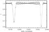 |
Fig. 2 Blow-up of a section of the light-curve in Fig. 1. |
| In the text | |
|
Fig. 3 Sections of the phased light curve around minima. Left panel: primary minimum; right panel: secondary minimum. Δφ is the phase difference with respect to conjunction phase. The curves labeled with “a” are derived by phasing LC0; curves “b” after prewhitening with pulsations, with no correction for visibility during eclipse. Curve “c” of the right panel is prewhitened taking visibility into account (see text). |
| In the text | |
|
Fig. 4 Phased light curve of the eclipsing binary as residuals of the corrected harmonic fit, orbital overtones excluded. Phases are derived using the ephemeris of Eq. (1). |
| In the text | |
|
Fig. 5 Abundances of the primary (asterisks) and secondary (open circles) components in dex relative to the solar values. The dashed and dotted lines mark the [Fe/H] of the primary and secondary components, respectively. |
| In the text | |
|
Fig. 6 Upper two panels: phased RV shifts of KIC 3858884 components from KOREL. Filled circles: primary star. Filled squares: secondary star. Curves: PHOEBE fit. Second panel: fit residuals, with the same symbols. Lower two panels: the same after prewhitening with the two significant frequencies found in the residuals. |
| In the text | |
|
Fig. 7 Amplitude spectra, based on our complete dataset of 83 spectra. From top to bottom: original data, largest peak f1; f1 subtracted, largest peak f2; f1 and f2 subtracted. |
| In the text | |
|
Fig. 8 Upper panel: phased light curve of the eclipsing binary and the final fit with PHOEBE (full line, in red in the online version), inset: a blow-up around periastron phase showing the fit around periastron phases. Lower panel: fit residuals. |
| In the text | |
|
Fig. 9 Blow up of the PIKAIA results: cost function value vs. inclination (top left), secondary temperature (top right), and potentials (bottom panels). The minimum value is indicated by a gray (red in the electronic version) larger dot. |
| In the text | |
|
Fig. 10 Final amplitude spectrum of KIC 3858884 and, in the inset a blow-up of the same spectrum after prewhitening the two highest frequencies. The gray line (red in the online version) is the significance threshold, which is four times the local noise (computed on the residual spectrum with a box of 3 d-1). |
| In the text | |
|
Fig. 11 Distribution of differences among the detected frequencies (every frequency was subtracted from all the others and the plot is restricted to the positive values). For easier comparison, each histogram is normalized to the local maximum around 7 d-1. The black line refers to the whole set of 403 frequencies, the gray line to those with amplitude larger than 10-4. The histograms show that there is a preferred spacing around 2.3 d-1, which is clearly visible in both distributions. According to Breger et al. (2009), the spacing corresponds to spacing between radial modes. The multiples of the spacing are also indicated by dotted lines. |
| In the text | |
|
Fig. 12 Frequency spectrum in the γ Dor domain after prewhitening with the first twelve frequencies of Table B.1. The highest amplitude peak corresponds to f13 ≃ 18forb. The gray (red) line is the estimate of local noise by PERIOD04 (with a box of 0.2 d-1). The black dots denote the values used to derive the period spacing. The open circle denotes the frequency f193 = 1.2350 d-1, which according to that period spacing value has nf193 = 39. This last frequency is also very close to 32forb. |
| In the text | |
|
Fig. 13 Properties of the stellar models selected as explained in the text. In all panels different quantities are plotted as function of the model age, the symbol shape depends on the chemical composition, the grey symbols correspond to the primary star, the black ones to the secondary. Top left panel: Teff for both stars; top-right panel: the integral of the Brunt-Väisälä frequency for the secondary component; bottom left panel: the minimum and maximum excited frequency in the δ Sct domain for both stars (empty and full symbols denote, respectively, the minimum and maximum values); bottom right panel: the minimum and maximum excited frequency in the γ Dor domain for the secondary. |
| In the text | |
|
Fig. 14 Example of evolutionary tracks for a pair of stellar models fulfilling the constraints explained in the text, and with Y = 0.27, Z = 0.016 and αOV = 0.2. For this particular pair Teff,1 = 6860 K and Teff,2 = 6680 K, the requested difference in radius with similar masses is fulfilled thanks to a more evolved stage of the primary component. |
| In the text | |
Current usage metrics show cumulative count of Article Views (full-text article views including HTML views, PDF and ePub downloads, according to the available data) and Abstracts Views on Vision4Press platform.
Data correspond to usage on the plateform after 2015. The current usage metrics is available 48-96 hours after online publication and is updated daily on week days.
Initial download of the metrics may take a while.