© ESO, 2014

1. Introduction

Transiting hot Jupiters are highly valuable in the characterization study of planetary orbits, structures, and atmospheres. They orbit the host stars closely while they possess relatively large sizes and high masses, thereby producing strong transit and radial velocity signals, which together result in precise determination of the planetary system parameters, such as planetary mass, radius, surface gravity, orbital distance, and stellar density (e.g., Seager & Mallén-Ornelas 2003; Southworth et al. 2007). Based on these fundamental parameters, the planetary composition and internal structure could be investigated, offering insight into the planetary formation, evolution, and migration history (e.g., Guillot 2005; Guillot et al. 2006; Charbonneau et al. 2007; Fortney et al. 2007).

With high-incident irradiation from the host stars, transiting hot Jupiters also play a crucial role in planetary atmospheric characterization. Through observations of primary transits, transmission spectrum can be constructed by measuring the transit depths at different wavelengths, which carries information of planetary atomic (e.g., Na, K) and molecular (e.g., H₂O, CH₄, CO) absorption features when the stellar lights are transmitted in the planetary day-night terminator region (Seager & Sasselov 2000; Fortney et al. 2008, 2010, etc.). In a similar way, the thermal emission spectrum can be obtained by measuring the occultation depths (approximately the planet-to-star flux ratios) during secondary eclipses (i.e., occultations), which puts constraints on both the chemical composition and temperature structure of the day-side atmosphere (Burrows et al. 1997, 2006, 2008a; Burrows & Sharp 1999; Fortney et al. 2008; Madhusudhan & Seager 2009, etc.).

Abundant observations have been performed to characterize the atmospheres for dozens of hot Jupiters in these two aspects (see the review by Seager & Deming 2010). However, very few hot Jupiters have been studied in both aspects, which are complementary and could potentially constrain the origin of thermal inversions (e.g., Hubeny et al. 2003; Burrows et al. 2007; Fortney et al. 2008; Madhusudhan & Seager 2010), since the absorbers that cause thermal inversions also imprint their spectral signatures on transmission spectra. This kind of study has started to emerge on some typical cases of hot Jupiters, for example, HD 189733b (Pont et al. 2013), WASP-12b (Swain et al. 2013), and WASP-19b (Bean et al. 2013).

WASP-43b, a hot Jupiter orbiting a K7V star every 0.81 days, was first discovered by Hellier et al. (2011). It has the smallest orbital distance to its host star among the Jupiter-size planets. The host star is active as indicated by the presence of strong Ca H+K emission. Gillon et al. (2012) significantly improved the WASP-43 system parameters based on 20 transits observed with the 60 cm robotic TRAPPIST telescope and three transits with the 1.2 m Euler Swiss telescope. The deduced planetary mass (2.034 ± 0.052 M_Jup) and radius (1.036 ± 0.019 R_Jup) indicate a high bulk density that favors an old age and a massive core. They also observed the occultations of WASP-43b at narrow bands with VLT/HAWK-I, resulting in a thermal emission detection at 2.09 μm (F_p/F_⋆ = 0.156 ± 0.014%) and a tentative detection at 1.19 μm (0.079 ± 0.032%). Blecic et al. (2014) performed atmospheric modeling based on their warm Spitzer detections at 3.6 μm (0.346 ± 0.012%) and 4.5 μm (0.382 ± 0.015%), in combination with the two ground-based near-infrared (NIR) detections of Gillon et al. (2012), which rules out a strong thermal inversion in the dayside atmosphere, and suggests inefficient day-night energy redistribution. Recently, Wang et al. (2013) have carried out occultation observations with the WIRCam instrument on the Canada-France-Hawaii telescope and detected the thermal emission in the H-band (0.103 ± 0.017%) and K_S-band (0.194 ± 0.029%). However, current data are still insufficient for constraining the chemical composition of WASP-43b’s atmosphere.

In 2011, we started a project to characterize hot-Jupiter atmospheres using the GROND instrument (e.g., Paper I on WASP-5b; Chen et al. 2013), which is able to do simultaneous multiband photometry. This technique now has been performed on several transiting planets to investigate their atmospheres (de Mooij et al. 2012; Southworth et al. 2012; Mancini et al. 2013a,b,c; Nikolov et al. 2013; Fukui et al. 2013; Copperwheat et al. 2013; Nascimbeni et al. 2013). Among our targets, WASP-43b is favorable for observation because of its large transit depth ~2.5% and high incident irradiation ~9.6 × 10⁸ erg s^-1 cm^-2 (Gillon et al. 2012). If zero albedo and zero day-to-night heat redistribution are assumed, an equilibrium temperature of 1712 K is derived. We aim to construct a broad-band transmission spectrum for WASP-43b and also to detect its NIR thermal emission.

This paper is organized as follows. Section 2 summarizes the transit and occultation observations, as well as the data reduction. Section 3 describes the process of transit and occultation light-curve modeling, including the reanalysis of light curves obtained by amateur astronomers. Section 4 reports the newly derived orbital ephemeris and fundamental physical parameters, and presents discussion on WASP-43b’s atmospheric properties. Section 5 gives the overall conclusions.

2. Observations and data reduction

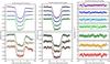Fig. 1 Primary transit light curves of WASP-43b as observed with the GROND instrument mounted on the ESO/MPG 2.2 m telescope. In each panel, transit light curves of g′r′i′z′JHK are shown from top to bottom. Left panel shows light curves that are normalized by the reference stars. Middle panel shows baseline-corrected light curves that are binned every 2 min for display purposes (see Sect. 3.1 for baseline correction). Right panels show the best-fit light-curve residuals, also binned every 2 min. Best-fit models for all panels are overlaid in solid or dashed lines.

We observed one primary transit and one secondary eclipse event of WASP-43b with the GROND instrument mounted on the MPG/ESO 2.2 m telescope at La Silla in Chile. GROND is an imaging instrument primarily designed for investigating gamma-ray burst afterglows and other transients simultaneously in seven bands: Sloan g′, r′, i′, z′ and NIR J, H, K (Greiner et al. 2008). The light goes through dichroics and is split into optical and NIR arms and further into seven bands. The optical arm employs backside-illuminated 2048 × 2048 E2V CCDs without antiblooming structures, which have a field of view (FOV) of 5.4 × 5.4 arcmin², a pixel scale of , and store data in FITS file with four extensions. The NIR arm employs 1024 × 1024 Rockwell HAWAII-1 arrays with an FOV of 10 × 10 arcmin² and a pixel scale of 0.̋60, which place data of three bands side by side in a single FITS file. The GROND guide camera is placed outside of the main GROND vessel, resulting in a guiding FOV which is 23′ south of the scientific imaging FOV. Taking the different FOV scales between optical and red arms, the orientation of guiding system, and the inclusion of as many reference stars as possible into account, a compromise between these factors is necessary when designing the observing strategy. Nevertheless, GROND is still a potentially good instrument for exoplanet observations, since it has very few moving parts and the capability of multiband observations with broad wavelength coverage.

The observing strategies for both transit and occultation were the same. We heavily defocused the telescope during both observations in order to spread the light of stars onto more pixels, which as a result could reduce the noise arising from the small number of pixels and avoid reaching the nonlinear regime. When achievable, we did sky measurements both before and after the science time series, which were designed in a 20-position dither pattern around the scientific FOV. According to the experience that we had in the observations of WASP-5b (Chen et al. 2013, Paper I), the staring mode is more stable and introduces fewer instrumental systematic effects than nodding mode. Therefore, for the WASP-43b observations, we made the telescope stare at the target during the three-hour-long science time series. The observations were carried out in the g′r′i′z′JHK filters simultaneously. The final observing duty cycle is determined by the compromise between the integration times of the optical arm and NIR arm, since they are not fully independent when in operation. The summary of both transit and occultation observations are listed in Table 1.

2.1. Transit observation

The transit event was observed on January 8, 2012, from 05:24 to 08:21 UT, which covered ~50 min both before expected ingress and after expected egress (see Fig. 1). This night had high relative humidity, ranging from 40% to 60%. The moon was illuminated by 99%, with a minimum distance of 65° to WASP-43. The airmass was well below 1.30. Although the telescope was heavily defocused, the radius of the donut-shaped point spread function (PSF) ring varied by as much as during the observation, indicating that the seeing was not very stable and that it had an evident impact on our PSF. The observation was in a good autoguiding status thanks to a bright star in the guiding FOV. We did sky measurements only before the science time series because the morning twilight had begun at the end of the observation. For the science time series, the optical bands were integrated for 90 s in fast read-out mode simultaneously, and 81 frames were recorded, resulting in a duty cycle of ~69%. The NIR bands were integrated with eight subintegrations of three seconds, which were averaged together before readout. Two hundred forty-four frames were recorded in the NIR, resulting in a duty cycle of ~56%.

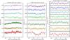Fig. 2 Occultation light curves of WASP-43b as observed with GROND. In each panel, shown from top to bottom are the occultation light curves of g′r′i′z′JHK. Left panel: light curves that are normalized by the reference stars. Middle panel: baseline-corrected light curves that are binned every 8 min for display purpose (see Sect. 3.1 for baseline correction). Right panels: best-fit light-curve residuals, also binned every 8 min. Best-fit models for all panels are overlaid in solid or dashed lines. The occultation depth is detected in the K-band (0.197 ± 0.042%) and marginally detected in the i′-band (0.037 $\begin{array}{c}\mathrm{+}\mathrm{0.023}\\ -0.021\end{array}$%).

2.2. Occultation observation

The occultation event was observed on March 3, 2012, from 02:52 to 05:59 UT, which covered ~70 min before expected ingress and ~40 min after expected egress (see Fig. 2). Relative humidity for this night was also high (~45%), and the moon was illuminated by 69% with a minimum distance of 63° to WASP-43. The airmass was below 1.20 for the whole event. The resulting PSF donut ring size was stable out-of-eclipse, while it varied a lot during the eclipse, which was caused by the sudden jumps of poor seeing. We did sky measurements both before and after the science observation. The optical bands were integrated with 90 s in fast read-out mode, while the NIR bands were integrated with four subintegrations of 4.5 s. In the end, we collected 98 frames for the optical and 389 frames for the NIR, translating into a duty cycle of 78% and 63%, respectively.

2.3. Data reduction

Both sets of observations were reduced in a standard way with our IDL¹ codes, which largely make use of NASA IDL Astronomy User’s Library². Calibration for the optical data includes bias subtraction and flat division. The master frames for both were created from median combination of individual measurements. The twilight sky flat measurements were star-masked and normalized before median combination.

For the NIR data, the calibration is a little more complicated owing to an electronic odd-even readout pattern along the X-axis. The calibration includes dark subtraction, readout pattern removal, and flat division. The master frames for dark, twilight sky flat and sky measurements were created through median combination as well, except that the sigma-clipping filter was applied when necessary. After the dark was corrected, each image was smoothed with a median filter and compared to the unsmoothed one. The amplitudes of the readout pattern were determined by differentiating median value of each column to the overall median level, and were then corrected in the original dark-subtracted images. The flat field was corrected after the removal of this pattern.

According to our experience on other targets (e.g., Chen et al. 2013), sky subtraction might result in light curves of slightly better precision. In this approach, a sky model is created and subtracted for each individual science frame by optimally combining the scaled before-and-after science sky measurements. This technique is not able to remove temporal variations, but should be helpful for removing spatial variations. However, this is not the case for this study. We found no improvement in the data set by applying the sky subtraction technique, so we decided to perform our analysis on the data set without sky subtraction.

After these calibrations, we employed the IDL/DAOPHOT package to perform aperture photometry on WASP-43, as well as on nearby comparison stars of similar brightness. The location of each star was determined by IDL/FIND, which calculates the centroid by fitting Gaussians to the marginal x, y distributions. This centroid algorithm was applied on the Gaussian-filtered images that had lower resolution, in which the irregular donut-shaped PSFs became nearly Gaussian after proper convolution. We recorded the FWHM of each star by masking out the central region of the original donut and fitting a Gaussian to the donut wing. The time series of each star was self-normalized with its out-of-transit flux level. We then carefully chose the best comparison-star ensemble in each band to correct the first-order atmospheric effect on the WASP-43 time series in the following way: various combinations of comparison stars were experimented with. The ensemble that leaves WASP-43 with the least light-curve O–C residuals was chosen. To find the optimal photometry, 40 apertures were laid on the optical images in steps of one pixel, each with ten sky annulus sizes in steps of two pixels, while 30 apertures were laid on the NIR images in steps of 0.5 pixel, each with ten sky annulus sizes in steps of one pixel. This resulted in 400 and 300 datasets with different aperture settings for the optical and NIR, respectively, and the one that leaves WASP-43 with the least amount of light-curve O–C scatter was adopted. Table 1 lists the number of reference stars in use and the final apertures for photometry.

Finally, we extracted the observation time of each frame. In this process, we centered the time of each frame based on its actual total integration. This UTC time was then converted to Barycentric Julian Date in the Barycentric Dynamical Time standard (BJD_TDB) using the IDL procedure written by Eastman et al. (2010).

3. Light curve analysis

3.1. Light curve modeling

As shown in the lefthand panels of Figs. 1 and 2, the reference-corrected light curves still exhibit systematics that are correlated with instrumental parameters or atmospheric conditions (star’s location on the detector, seeing, etc.). To model these light curves properly, we chose to fit the data with models composed of two components: $\mathit{F}\mathrm{\left(}\mathrm{mod}\mathrm{\right)}\mathrm{=}\mathit{E}\mathrm{\left(}{\mathit{p}}_{\mathit{i}}\mathrm{\right)}\mathit{B}\mathrm{\left(}\mathit{x,y,z,s,t}\mathrm{\right)}\mathit{.}$(1)The first component is the analytic light curve model (Mandel & Agol 2002), representing the transit or occultation signal itself. For the transit event, a quadratic limb darkening law is adopted: ${\mathit{I}}_{\mathit{\mu }}\mathit{/}{\mathit{I}}_{\mathrm{1}}\mathrm{=}\mathrm{1}\mathrm{-}{\mathit{u}}_{\mathrm{1}}\mathrm{(}\mathrm{1}\mathrm{-}\mathit{\mu }\mathrm{)}\mathrm{-}{\mathit{u}}_{\mathrm{2}}\mathrm{(}\mathrm{1}\mathrm{-}\mathit{\mu }\mathrm{)}2$(2)where I is the intensity and μ = cosθ (θ is the angle between the emergent intensity and the line of sight). We calculate the two theoretical coefficients u₁ and u₂ by bilinearly interpolating in the Claret & Bloemen (2011) table, in which the effective temperature T_eff = 4520 ± 120 K, the surface gravity log g_⋆ = 4.645 ± 0.011, and the metallicity [Fe/H]  = −0.01 ± 0.12 are taken from Gillon et al. (2012), while the microturbulence ξ_r = 0.5 ± 0.3 km s^-1 is from Hellier et al. (2011). The resulting values with uncertainties are set as Gaussian priors (GP; see Eq. (4)) in the subsequent fitting process and listed in Table 2. Thus this theoretical model E(p_i) contains six free parameters: the orbital inclination i, the planet-to-star radius ratio R_p/R_⋆, the scaled semi-major axis a/R_⋆, the midtransit point T_mid, the limb-darkening coefficients u₁ and u₂, while the period P is fixed at the literature value (or updated ephemeris iteratively, see Sect. 4.1). The eccentricity e is fixed to zero since it cannot be determined by a single transit.

For the occultation event, E(p_i) becomes $\mathit{E}\mathrm{(}{\mathit{T}}_{\mathrm{occ}}\mathit{,}{\mathit{F}}_{\mathrm{p}}\mathit{/}{\mathit{F}}_{\mathit{\star }}\mathrm{)}\mathrm{=}\mathrm{1}\mathrm{-}\frac{{\mathit{\lambda }}_{\mathrm{e}}}{\mathrm{1}\mathrm{+}\mathrm{(}{\mathit{F}}_{\mathrm{p}}\mathit{/}{\mathit{F}}_{\mathit{\star }}{\mathrm{)}}^{-1}}$(3)where λ_e refers to Eq. (1) in Mandel & Agol (2002) in the case of uniform source without limb darkening. This model has two free parameters: the mid-occultation time T_occ and the planet-to-star flux ratio F_p/F_⋆, while other parameters are fixed at values inherited from the transit event.

The second component is the baseline correction function, which is used to correct the instrumental and atmospheric systematics, including the effects of the star’s location on the detector (x, y), PSF donut-ring size s, airmass z, and time sequence t. We search for the best-fit parameters by minimizing the chi-square: ${\mathit{\chi }}^{\mathrm{2}}\mathrm{=}\sum _{\mathit{i}\mathrm{=}\mathrm{1}}^{\mathit{N}}\frac{\mathrm{\left[}{\mathit{F}}_{\mathit{i}}\mathrm{\right(}\mathrm{obs}\mathrm{)}\mathrm{-}{\mathit{F}}_{\mathit{i}}\mathrm{(}\mathrm{mod}\mathrm{)}{\mathrm{]}}^{\mathrm{2}}}{{\mathit{\sigma }}_{\mathit{F,i}}^{\mathrm{2}}\mathrm{\left(}\mathrm{obs}\mathrm{\right)}}\mathrm{+}\mathrm{GP}\mathit{.}$(4)We select the best baseline model for each band based on the Bayesian information criteria (BICs, Schwarz 1978): BIC = χ² + klog (N), where k is the number of free parameters and N the number of data points. The chosen baselines with their derived coefficients for both nights are listed in Appendix A.

To determine the probability distribution function (PDF) for each parameter, we employ the Markov chain Monte Carlo (MCMC) technique with the Metropolis-Hastings algorithm with Gibbs sampling (see e.g., Ford 2005, 2006). Instead of perturbing the baseline coefficients, we follow the approach of Gillon et al. (2010), in which these coefficients are solved by the singular value decomposition algorithm (SVD, Press et al. 1992). At each MCMC step, a jump parameter is randomly picked out, and the analytic light curve model E(p_i) is divided from the light curve. The baseline coefficients are then determined by linear least square minimization using SVD. If the resulting χ² is less than the previous χ², this jump is directly accepted. However, if it is larger, we still accept it with a probability of exp(−Δχ²/2). Before a chain starts, we optimize the step scale using the method proposed by Ford (2006) so that the acceptance rate is ~0.44. After several chains are completed, we do Gelman & Rubin (1992) statistics to check whether they are well mixed and converged. In the end, we discard the first 10% links of each chain and calculate the median value, along with the 15.865% and 84.135% level of the marginalized distribution of the remaining links, which are recorded as the best-fit parameters and 1σ lower and upper uncertainties.

Since the photometric uncertainties sometimes do not reflect the actual properties of the light curve data points, owing to either under-/overestimation of noise or to time-correlated noise, we performed rescaling on the uncertainties in two steps. For each MCMC fitting process, we always initially ran several chains of 10⁵ links on the data with original photometric uncertainties. In the first step of rescaling, we calculated the reduced ${\mathit{\chi }}_{\mathit{\nu }}^{\mathrm{2}}$ for the best-fit model, and recorded the first rescaling factor ${\mathit{\beta }}_{\mathit{\chi }}\mathrm{=}\sqrt{{\mathit{\chi }}_{\mathit{\nu }}^{\mathrm{2}}}$ in order to force the best fit to have a reduced chi-square equal to unity. In the second step, we followed the approach of Winn et al. (2008) to account for the effect of time-correlated red noise, in which two methods were utilized. In the “time-averaging” (TA) method (see e.g., Pont et al. 2006), red noise remains unchanged while white noise scales down with larger binning (see Fig. 3). Standard deviations for the best-fit residuals without binning and with binning in different time resolutions, ranging from ten minutes up to the duration of ingress/egress, were calculated to estimate this factor: ${\mathit{\beta }}_{\mathrm{TA}\mathit{,N}}\mathrm{=}\frac{{\mathit{\sigma }}_{\mathit{N}}}{{\mathit{\sigma }}_{\mathrm{1}}}\sqrt{\frac{\mathit{N}\mathrm{(}\mathit{M}\mathrm{-}\mathrm{1}\mathrm{)}}{\mathit{M}}}$(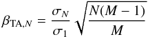5)where σ_N is the standard deviation of residuals binned in N points, and M is the number of bins. The final β_TA is taken to be the median value of several of the largest β_TA,N, from which outliers could be removed, while the information of the red noise component remains unchanged. In the “prayer-bead” (PB) method (see e.g., Southworth 2008), the shape of time-correlated noise was preserved. The best-fit residuals were shifted cyclicly from the ith to the i+1th position and added back to the best-fit model, while off-position data points at the end were wrapped back to the beginning. This was repeated in the opposite direction as well, so that 2N − 1 synthetic light curves were created and modeled. The ratio between uncertainties derived from this process and the original MCMC process was recorded as β_PB. Finally, we adopted the red noise factor as β_r = max(β_TA,β_PB,1). We then rescaled the original uncertainties by β_χ × β_r (see corresponding entries in Tables 1 and 3), and ran several more chains of 10⁶ links to find the final best-fit parameters.

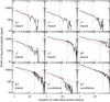Fig. 3 Standard deviation of light-curve O–C residuals binned in different time resolutions, showing the level of time-correlated noise. Red dashed line indicates the expected Poisson-like noise, i.e., standard deviation of unbinned O–C residuals over square-root of N. Vertical dotted line shows corresponding ingress/egress duration. The number following the filter name indicates either primary transit (1) or occultation (2).

3.2. Fitting of transit light curves

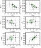Fig. 4 Correlations between pairs of jump parameters for the transit light curves. Black circles with error bars are the results from individual analysis (Method 1) on the seven-band light curves, while contours indicate the joint probability distribution function (PDF) from global joint analysis with common radius (Method 2). Both methods have consistent correlation.

Our seven-band transit light curves were obtained simultaneously, and they covered a wide wavelength range from the optical to the NIR. While most inferred physical properties should mainly be the same in different bands, the probed apparent planetary “radius” could depend on wavelength. Therefore we adopted three methods of MCMC analysis to determine the system parameters and to investigate their deviations:

• Method 1: individual analysis. The seven transit light curveswere fitted individually, in which i, a/R_⋆, R_p/R_⋆ and T_mid were obtained for eachlight curve.

• Method 2: global joint analysis with common radius. The seven transit light curves were jointly fitted, in which all the light curves shared the same i, a/R_⋆, R_p/R_⋆, and T_mid.

• Method 3: global joint analysis with wavelength-dependent radius. The seven transit light curves were jointly fitted, where all the light curves shared the same i, a/R_⋆, and T_mid, while R_p/R_⋆ was allowed to vary from filter to filter.

In Method 1, we tried to characterize the light curves individually, so that the variation in derived parameters from filter to filter can be investigated. Overall, the derived parameters are consistent with each other. The standard deviations of individual i and a/R_⋆ are well below their average uncertainties, while those of R_p/R_⋆ and T_mid are less than twice their average uncertainties. Strong correlation between i and a/R_⋆ can be seen (see the data points with error bars in Fig. 4), and both of them are correlated with R_p/R_⋆. Only T_mid is independent of other parameters. Most red noise factors come from the time-averaging method, except in the g′- and H-bands. These factors are very close to unity in the optical, indicating that the level of red noise is low. It could also be a result of relatively long exposure time (90 s), which keeps the cadence from being frequent enough to reflect the feature of red noise. The level of time-correlated noise in the NIR seems obvious even with visual inspection, especially the dip between +50 and +80 min as shown in Fig. 1, thus resulting in larger rescaling factors. We estimated the standard deviation of best-fit residuals in two-minute intervals to show the quality of the light curve, which can be directly compared to Gillon et al. (2012). We achieved a scatter of ~0.05–0.08% in the optical and ~0.11–0.13% in the NIR in two-minute intervals, which correspond to a range of ~2.1–4.5 and ~6.2–8.7 times the photon noise limit, respectively. For comparison, Gillon et al. (2012) reached accuracies ~0.11–0.15% in their optical transit light curves using 60 cm and 1.2 m telescopes, and ~0.04–0.05% in their NIR occultation light curves using an 8.2 m telescope.

In Methods 2 and 3, we tried to obtain transit parameters from a global view, in which we can avoid introducing extra variations from the correlation between parameter pairs (e.g., i and a/R_⋆). The differences between Methods 2 and 3 depend mainly on whether the apparent planetary radius is wavelength-dependent. We also calculated the weighted average of R_p/R_⋆ for Method 3 in the same way as we did in Method 1.

Results from these three methods agree very well with each other within their error bars. Since physically the probed atmospheric depth could be different in different bands owing to either clouds/hazes or atomic/molecular absorption, we decided to report results from Method 3 as our final results. The red noise factors are greater in the cases of global joint analysis, which is expected since time-correlated noise is coupled with light curves, and individual analysis has more flexibility in the modeling. The red noise factors of Method 3 are shown in Table 1, while those of Method 1 are shown in Table 3.

3.3. Fitting of occultation light curves

Given the modest light-curve quality, we fitted the seven occultation light curves by fixing the mid-occultation time T_occ and common transit parameters at known values and by only setting F_p/F_⋆ as the free parameter. Values of a/R_⋆, R_p/R_⋆, and i were obtained from the global joint analysis on our transit light curves (Method 3). The value of T_occ was calculated from T_occ = T₀ + (N + φ)P, where N = 67 and φ = 0.5002 ± 0.0004. The midoccultation phase φ was taken from Blecic et al. (2014), which was precisely determined by the joint analysis of Spitzer 3.6 μm and 4.5 μm occultation light curves. We only detected or marginally detected the occultation signals in the K- and i′-bands.

The flux ratios detected in the K- and i′-bands are 0.197 ± 0.042% and 0.037 $\begin{array}{c}\mathrm{+}\mathrm{0.023}\\ -0.021\end{array}$%, respectively. Our i′-band detection is marginal with 1.8σ significance. Our K-band detection agrees within 1σ with the value of 0.156 ± 0.014% obtained with VLT/HAWK-I in the 2.09 μm narrow band (Gillon et al. 2012), and agrees well with the value of 0.194 ± 0.029% obtained with CFHT/WIRCam in the K_S-band (Wang et al. 2013). The time-correlated noise level is low for both K- and i′-bands as shown in Fig. 3. We achieved a scatter of 1425 ppm and 604 ppm in two-minute intervals for the K- and i′-bands, with the corresponding estimated photon noise limits of 2.1 × 10^-4 and 1.9 × 10^-4, respectively.

We also tried freely fitting T_occ in addition to F_p/F_⋆ for the K- and i′-bands, so as to test the dependence of flux ratio on mid-occultation time. This resulted in F_p/F_⋆ = 0.203 ± 0.036% and ${\mathit{F}}_{\mathrm{p}}\mathit{/}{\mathit{F}}_{\mathit{\star }}\mathrm{=}\mathrm{0.03}{\mathrm{7}}_{-0.021}^{\mathrm{+}\mathrm{0.023}}$%, respectively. As shown in Fig. 5, while the i′-band T_occ is not well constrained, the K-band T_occ occurs on an offset phase around $\mathit{\phi }\mathrm{=}\mathrm{0.490}{\mathrm{7}}_{-0.0027}^{\mathrm{+}\mathrm{0.0036}}$ (i.e., an offset of –10.9 min to φ = 0.5002). Since both Spitzer and high-precision ground-based occultation observations have ruled out an eccentric orbit for WASP-43b (Gillon et al. 2012; Blecic et al. 2014; Wang et al. 2013), we speculate the offset of our T_occ arising from contamination of instrumental systematics. However, we note that the occultation depths do not strongly depend on phase. The measured depths remain nearly constant within 1σ when T_occ varies from phase 0.48 to 0.51.

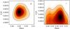Fig. 5 Correlation between mid-occultation time (converted to phase for display purpose) and flux ratio for the K- and i′-bands derived from the MCMC analysis. Three contour levels indicate the 68.3% (1σ), 95.4% (2σ), and 99.7% (3σ) confidence levels, respectively.

3.4. Fitting of mid-transit times

We performed another individual analysis on the seven transit light curves in order to investigate the central transit times under the control of common system parameters. We adopted i, a/R_⋆, and R_p/R_⋆ determined in the global joint analysis (Method 3), and imported them as Gaussian priors in this analysis. Only T_mid was allowed to freely float throughout this modeling. This results in seven measurements on the same epoch. As shown in Fig. 6, the seven central times are not exactly the same. The standard deviation of their best-fit values is ~1.3 times their mean uncertainties. Compared to the uncertainty-weighted average, the r′-, i′-, H-, K-bands deviate less than 1σ, the z′-, J-bands deviate less than 2σ, while the g′-band deviates ~2.2σ.

We repeated this analysis with different baseline models to examine whether this deviation was caused by detrending. However, even when we forced all the light curves to have the same simplest model (normalization factor plus a slope, i.e. c₀ + c₁t), we could see a similar trend. Therefore, if this deviation comes from an imperfect light curve shape, we cannot correct it by introducing baseline correction. Another possibility is that the uncertainties of these central times are still underestimated. Considering that all the timings deviate from the average by much less than 2σ (except g′), this deviation is not significant.

We also analyzed the amateur transit light curves obtained from the TRESCA Project³ (Poddaný et al. 2010), which is used in the investigation of transit timing variations (TTVs) effect in Sect. 4.1. We discarded 15 out of 42 available light curves to date (August 2013), because of either partial transits or very poor data quality (with a scatter in best-fit residuals larger than 1%) or asymmetric transit shape caused by strong visible time-correlated noise. Since most of these data lack the instrumental parameters, while some of them even do not have measurement uncertainties, the instrumental systematics that might affect the transit shape can hardly be corrected. To determine the central transit times more robustly, we replaced our fitting statistic (i.e., χ²) with the wavelet-based likelihood function proposed by Carter & Winn (2009), in which we assume that the time-correlated noise varies with a power spectral density of 1/f at frequency f. The jump rule is the same, except that the likelihood increases with higher probability. We converted the time stamps of TRESCA light curves into BJD_TDB and adopted i, a/R_⋆, and R_p/R_⋆ as Gaussian priors from our analysis described in Sect. 3.2. This resulted in uncertainties for the TRESCA central transit times that are ~20–270% (on average 80%) longer than those originally listed in the TRESCA website. The newly determined central transit times for the TRESCA light curves are shown in Table 4. As a comparison, the timings of our seven transit light curves would have been enlarged ~10% using this wavelet-based analysis. However, to have a direct comparison with Gillon et al. (2012) for our transit light curves, we chose the timings from the χ²-based analysis as the final values.

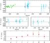Fig. 6 Transit timing O–C residuals for WASP-43b. In the top panel, green circles show timings from Gillon et al. (2012) (with epoch less than –200), blue squares show timings from TRESCA (with epoch longer than –10, see Sect. 3.4 for the reanalysis process), while red star shows our weighted average timing value (at epoch 0), where the error bar indicates the standard deviation of our seven filters. Middle panels: a zoom-in view of the transit timings obtained after epoch –10. Bottom panel: our seven-filter timings. The dashed line refers to the linear regression, while the dotted line represents a quadratic fit.

4. Results and discussion

4.1. Period determination

In addition to our seven timing measurements on one transit and 27 reanalyzed timings from TRESCA, we also collected the 23 timings listed in Table 6 of Gillon et al. (2012). We fitted a linear function to these 57 timings by minimizing χ²: ${\mathit{T}}_{\mathrm{c}}\mathrm{\left(}\mathit{E}\mathrm{\right)}\mathrm{=}{\mathit{T}}_{\mathrm{c}}\mathrm{\left(}\mathrm{0}\mathrm{\right)}\mathrm{+}\mathit{EP}$(6)in which E is the epoch, and the epoch number of our observation was set as 0. From the fitting we obtained a new transit ephemeris of T_c(0) = 2 455 934.792239 ± 0.000040 (BJD_TDB) and an improved orbital period of P = 0.81347437 ± 0.00000013 days. This new period is four times more precise than the one in Gillon et al. (2012). We show the O–C diagrams in Fig. 6 and list all the newly determined timing data in Table 4.

This fit has a χ² = 139.68 with 55 degrees of freedom (d.o.f.), resulting in a reduced chi-square ${\mathit{\chi }}_{\mathit{\nu }}^{\mathrm{2}}\mathrm{=}\mathrm{2.59}$. This indicates a poor fit by linear function. However, the standard deviation for the best-fit residuals is 52.6 s, while the median uncertainty for individual timings is 30.2 s. From this view, the significance of TTV is low. We examined all the timings and found that four epochs (−375, −347, −288, and −256) deviating more than 3σ level lead to this large ${\mathit{\chi }}_{\mathit{\nu }}^{\mathrm{2}}$, all of which come from Gillon et al. (2012). Discarding these four epochs would result in a lower value ${\mathit{\chi }}_{\mathit{\nu }}^{\mathrm{2}}\mathrm{=}\mathrm{1.62}$. We also note that, in the experiment of Sect. 3.4, the wavelet-based analysis produces on average 10% larger uncertainties than our time-averaging and prayer-bead methods. Considering that Gillon et al. (2012) performed a similar analysis to ours that is based on the timing-averaging method alone, it is likely that this poor fit arises from underestimated timing uncertainties.

Blecic et al. (2014) tried to fit all the available timings and to estimate the decay rate using an quadratic ephemeris model (Adams et al. 2010): ${\mathit{T}}_{\mathrm{c}}\mathrm{\left(}\mathit{E}\mathrm{\right)}\mathrm{=}{\mathit{T}}_{\mathrm{c}}\mathrm{\left(}\mathrm{0}\mathrm{\right)}\mathrm{+}\mathit{EP}\mathrm{+}\mathit{\delta P}\mathrm{\ast }\mathit{E}\mathrm{(}\mathit{E}\mathrm{-}\mathrm{1}\mathrm{)}\mathit{/}\mathrm{2.}$(7)They obtained a result strongly favoring this model over the linear one. Since their results were based on the original TRESCA timings with underestimated uncertainties, we decided to repeat the same quadratic fit, which had a result of T_c(0) = 2 455 934.792262 ± 0.000041, P = 0.81347399 ± 0.00000022 days, and δP = (−2.2 ± 1.1) × 10^-9 days orbit^-2. This δP translates into a Ṗ =  −0.09 ± 0.04 s year^-1, which is seven times smaller than in Blecic et al. (2014). This quadratic fit has aBIC of 147.36, which is almost the same as for the linear fit (BIC = 147.69). Therefore we can conclude that a quadratic model does not improve the fit of ephemeris.

As a conclusion, we prefer no evidence for significant TTV within the current dataset. The current TTV rms of 52.6 s roughly corresponds to a timing deviation caused by a perturber with a mass of 2.17 M_⊕ in the 2:1 resonance according to the relationship derived by Agol et al. (2005).

4.2. Physical parameters

To determine the physical parameters for the WASP-43 system, we made use of the output PDFs from our MCMC analysis of the transit light curves, stellar evolutionary tracks, and the RV semi-amplitude. We first derived a set of parameters that simply depended on the light curve, such as transit duration, ingress/egress duration, and mean stellar density, using the formulae from Seager & Mallén-Ornelas (2003). By adopting the RV semi-amplitude value (in the form of ${\mathit{K}}_{\mathrm{2}}\mathrm{=}\mathit{K}\sqrt{\mathrm{1}\mathrm{-}{\mathit{e}}^{\mathrm{2}}}{\mathit{P}}^{\mathrm{1}\mathit{/}\mathrm{3}}$) from Gillon et al. (2012), we were able to derive the planetary surface gravity (Southworth et al. 2007).

We then determined the stellar mass and age by interpolating in the stellar evolutionary tracks using the MCMC process. Since photometric measurements are independent of spectoscopic measurements that provide stellar effective temperature T_eff and metallicity [Fe/H], it is a good complement to the determination of stellar mass. To have a direct comparison with Gillon et al. (2012), we adopted the Geneva stellar evolutionary tracks (Mowlavi et al. 2012), and interpolated them into finer grids. The mass interpolation was performed in the [${\mathit{\rho }}_{\mathrm{\ast }}^{\mathrm{-}\mathrm{1}\mathit{/}\mathrm{3}}$, T_eff] plane by MCMC, in which T_eff and [Fe/H] were obtained from Gillon et al. (2012) and were randomly generated from Gaussian distributions, while ${\mathit{\rho }}_{\mathrm{\ast }}^{\mathrm{-}\mathrm{1}\mathit{/}\mathrm{3}}$ was taken from the a/R_⋆ chains derived in our previous global joint analysis. At each step, the link [${\mathit{\rho }}_{\mathrm{\ast }}^{\mathrm{-}\mathrm{1}\mathit{/}\mathrm{3}}$, T_eff] was put onto the tracks according to [Fe/H]. Interpolation was bilinearly performed among mass tracks and isochrones. Links that were off tracks or older than 12 Gyr were discarded. After this MCMC process, we derived a stellar mass of 0.713 $\begin{array}{c}\mathrm{+}\mathrm{0.018}\\ -0.021\end{array}{\mathit{M}}_{\mathrm{\odot }}$ and a poorly constrained age of 4.4 $\begin{array}{c}\mathrm{+}\mathrm{3.7}\\ -2.4\end{array}$ Gyr for WASP-43. The posterior distributions of T_eff (4536 $\begin{array}{c}\mathrm{+}\mathrm{98}\\ -85\end{array}$ K) and [Fe/H] (0.01 $\begin{array}{c}\mathrm{+}\mathrm{0.10}\\ -0.09\end{array}$) remain similar to input, whose best-fit values only shift slightly since our a/R_⋆ is slightly different from Gillon et al. (2012). Figure 7 shows the posterior distribution of this MCMC process. New stellar radius, orbital semi-major axis, and planetary radius were derived with this refined stellar mass value. Finally, the planetary mass was derived by solving the Eq. (25) of Winn (2010).

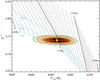Fig. 7 Stellar evolutionary tracks obtained from Mowlavi et al. (2012) to derive the stellar mass and age for WASP-43. Solid lines labeled with numbers show the basic tracks at solar abundance, while dotted lines show the interpolated tracks. Dashed lines indicate the isochrones. Contours overlaid on the distribution density map show the posterior distribution of links in our MCMC process, in which those with different metallicities are also included.

We obtained a mass of 2.029 $\begin{array}{c}\mathrm{+}\mathrm{0.035}\\ -0.040\end{array}$ M_Jup and a radius of 1.034 ± 0.014 R_Jup for WASP-43b, which correspond to a bulk density of 2.434 $\begin{array}{c}\mathrm{+}\mathrm{0.067}\\ -0.065\end{array}$ g cm^-3. This puts WASP-43b at the top of the list of dense hot Jupiters. Fortney et al. (2007) calculated groups of giant planet thermal evolution models, in which the mass-radius relationships are parameterized by age, core mass, and effective orbital distance. Assuming that WASP-43b is a hypothetical planet moving around the Sun, which receives the same flux as the actual planet, the effective orbital distance is calculated as a_⊕ = a(L_⋆/L_⊙)^− 1/2 = 0.0376 AU. According to the theoretical prediction, only models with an old age could explain current data. After interpolating in the theoretical models with a solar composition at 4.5 Gyr, we obtained theoretical planetary radii of 1.13 R_Jup, 1.07 R_Jup, and 1.01 R_Jup in the cases of core free, a 50 M_⊕ core, and a 100 M_⊕ core, respectively. Therefore, the current mass and radius for WASP-43b indicate a massive core inside this planet, and favor an old age that is consistent with the derived age from stellar evolutionary tracks.

4.3. Atmospheric properties

One of our primary goals observing both transit and occultation events is to probe the atmosphere of WASP-43b in a complementary way, since the atmosphere of both dayside and terminator region have been observed through these two events.

For the transit light curves, we did the reanalysis by fixing the values of i, a/R_⋆, and T_mid to those from the final global joint analysis (Method 3), while letting the limb-darkening coefficients float under the control of Gaussian priors. We derived the transit depth for each band and list them in Table 6. The resulting R_p/R_⋆ are slightly more precise than those determined in the global joint analysis, because the uncertainties of i, a/R_⋆, and T_mid were not propagated.Because we seek to derive the conditional distribution of transit depth in each band, the uncertainties arising from common parameters are not taken into account in the derived transmission spectrum.

For the occultation light curves, we also placed 3σ upper limits on the potential occultation depths in the other five bands in addition to the K- and i′-band detections, which are listed in Table 6.

4.3.1. A broad-band transmission spectrum

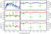Fig. 8 Model transmission spectra compared to observed transit depths which are derived from a single transit. In all panels, green circles with error bars show our measurements in the g′r′i′z′JHK bands, of which the horizontal error bars indicate the FWHM of each bandpass. Black dotted line shows a constant value of ${\mathit{R}}_{\mathrm{p}}^{\mathrm{2}}\mathit{/}{\mathit{R}}_{\mathit{\star }}^{\mathrm{2}}\mathrm{=}\mathrm{2.48}\mathrm{\%}$. Orange dashed line shows a Rayleigh scattering spectrum that is caused by a high-altitude haze. Three fiducial model spectra are shown for comparison, and their broad-band integrated values are displayed in yellow squares. The optical and NIR data are shown in separate panels with different scales for clarity. Top panels show a model with TiO/VO as the dominant opacity sources and a dayside-wide averaged (f = 1/2) pressure-temperature (P-T) profile. Middle and bottom panels show two models with Na and K as the dominant opacity sources. While the middle-panel model has a dayside-wide averaged P-T profile, the bottom-panel model has a planet-wide averaged P-T profile (f = 1/4). See Sect. 4.3.1 for detailed discussion.

We created a broad-band transmission spectrum by putting all the seven-band transit depths together with respect to wavelength. By fitting this observed “spectrum” to a flat straight line (see Fig. 8), we obtain a constant transit depth of ${\mathit{R}}_{\mathrm{p}}^{\mathrm{2}}\mathit{/}{\mathit{R}}_{\mathit{\star }}^{\mathrm{2}}\mathrm{=}\mathrm{2.48}\mathrm{\%}$ with χ² = 7.95 (6 d.o.f.), which indicates good agreement between the “spectrum” and a featureless line.The largest deviation comes from the i′-band (1.6σ), the H-band (1.5σ), and the K-band (1.6σ). We confirm that the deviation at these three bands does not arise from different detrending models for different bands, since this deviation shape still exists when forcing all seven light curves has the same baseline function. A flat featureless spectrum could indicate an atmosphere covered with high-altitude optically thick clouds.

The standard deviation of best-fit transit depth values is 0.051%. Although the insufficient precision (~0.02% and ~0.07% for the optical and NIR bands, respectively) prevents this variation from being significant, we still try to compare our “spectrum” to theoretical models, so as to examine whether a clear atmosphere could apply. Detailed atmospheric modeling is beyond the scope of this paper. Instead, we chose to generate fiducial atmospheric models based on the physical and orbital parameters of the WASP-43 system. The model atmosphere is computed using the approach described in Fortney et al. (2005, 2008), which uses the equilibrium chemistry mixing ratios from Lodders & Fegley (2002, 2006) and Lodders (2009) and adopts the opacity database from Freedman et al. (2008). The formation of clouds or hazes is not included. Three model transmission spectra (see the three panels in Fig. 8) are calculated following the method of Fortney et al. (2010), depending on how the atmospheric pressure-temperature (P-T) profile is dealt with and what optical opacity sources dominate. Model A has the P-T profile averaged over only the dayside (i.e., heat redistribution factor f = 1/2), the dominant opacities of which come from gaseous TiO/VO. In contrast, model B1/B2 has gaseous Na and K as the dominant opacity sources. While the P-T profile of B1 is similar to A, that of B2 is planet-wide averaged (i.e., f = 1/4). Broad-band model values are integrated from the synthetic transmission spectra over each bandpass of GROND.

We fit the observed “spectrum” to the three model spectra by shifting the models up and down, because the planetary base radius is unknown. The models are allowed to have different base radii. We find that they fit the observed “spectrum” equally well. The resulting χ² (6 d.o.f.) are 6.69, 7.62, and 7.36 for models A, B1, and B2, respectively. Fitting to fiducial atmospheric models only marginally improves from that to a flat line, and the dominant atmospheric opacity sources cannot be discerned.

We note that the best-fit transit depth values are in a decreasing trend from the g′-band to the K-band, indicating that Rayleigh scattering could exist in the upper atmosphere. A Rayleigh scattering signature has been observed in the transmission spectrum of HD 189733b obtained by several space-borne instruments (e.g., Lecavelier Des Etangs et al. 2008; Pont et al. 2008; Sing et al. 2011; Gibson et al. 2012; Pont et al. 2013). A recent work by Pont et al. (2013) summarized that HD 189733b has a high-altitude haze of condensate grains extending over at least five scale heights, which results in a Rayleigh scattering slope from UV into NIR. We follow the approach of Lecavelier Des Etangs et al. (2008, see their Eq. (1)) to construct a Rayleigh scattering spectrum for WASP-43b, in which MgSiO₃ (with a size of ~0.01 μm) is assumed as the haze condensate. By shifting the Rayleigh scattering spectrum to match our data, we obtain a good fit with χ² = 6.28 (6 d.o.f.). Therefore, an atmosphere with high-altitude hazes could also explain our observed “spectrum”. The Rayleigh scattering spectrum is shown in Fig. 8.

4.3.2. Detection of dayside flux in the K- and i′-bands

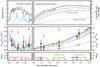Fig. 9 Dayside model spectra compared to the observed occultation depths. In the top panels, the left one displays the relative contributions of absorption (solid curves) and Rayleigh scattering (dotted lines). Two models of different opacity sources (TiO/VO in gray vs. Na/K in skyblue) are shown. The top right panel displays blackbody planetary dayside thermal emission spectra, with temperatures of 1784 K, 1439 K, 1712 K, and 1839 K, corresponding to the 2.09 μm brightness temperature TB and equilibrium temperatures Teq of three different heat redistribution factors. Middle panels show the planet-star flux ratios calculated based on the top panels. Our seven-band measurements are shown in red circles with error bars or arrows (3σ upper limit). Another two narrow-band measurements from VLT/HAWK-I (Gillon et al. 2012) and two broad-band measurements from CFHT/WIRCam (Wang et al. 2013) are shown with blue and green circles, respectively. Bandpass-integrated model values are plotted in symbols without error bars. Bottom panels show the filter transmission curves. See detailed discussion in Sect. 4.3.2.

We detected a flux ratio of 0.197 ± 0.042% in the GROND K-band and 0.037 $\begin{array}{c}\mathrm{+}\mathrm{0.023}\\ -0.021\end{array}$% in the GROND i′-band. Before comparing them to theoretical models, we first estimated their brightness temperatures. The planetary dayside thermal emission was simplified as a blackbody, while the stellar flux was interpolated from the Kurucz stellar models (Kurucz 1979) with the values of T_eff, log g, and [Fe/H] derived from this work. The K-band occultation detection is translated into a brightness temperature of 1878 $\begin{array}{c}\mathrm{+}\mathrm{108}\\ -116\end{array}$ K, while the i′-band detection corresponds to 2225 $\begin{array}{c}\mathrm{+}\mathrm{139}\\ -225\end{array}$ K.

With the equation ${\mathit{T}}_{\mathrm{eq}}\mathrm{=}{\mathit{T}}_{\mathrm{eff}\mathit{,}\mathrm{\ast }}\sqrt{{\mathit{R}}_{\mathit{\star }}\mathit{/}\mathit{a}}\mathrm{\left[}\mathit{f}\mathrm{\right(}\mathrm{1}\mathrm{-}{\mathit{A}}_{\mathit{B}}\mathrm{)}{\mathrm{]}}^{\mathrm{1}\mathit{/}\mathrm{4}}$ (where 1/4 ≤ f ≤ 2/3; Cowan & Agol 2011), we can infer the heat redistribution factor based on brightness temperature. However, the brightness temperatures at both K- and i′-bands exceed the maximum allowed equilibrium temperature 1839 K (when f = 2/3 and A_B = 0; i.e., heat is re-emitted instantly without redistribution). Given the large uncertainties of brightness temperature, our K-band still allows a heat redistribution factor of f ≥ 0.56 and a bond albedo of A_B ≤ 0.16 at 1σ level, which are indicative of very poor heat redistribution efficiency. For the i′-band, the brightness temperature exceeds the maximum temperature at the 1.7σ level. In contrast, an isothermal blackbody emission could provide a maximum flux ratio of 0.006% in the i′-band.

Since our K-band detection of thermal emission puts no other constraint than the VLT 2.09 μm narrow-band detection, detailed atmospheric modeling is again beyond the scope of this paper. Given that ground-available NIR bands contain only weak molecular features (Madhusudhan 2012), and the current data (including Warm Spitzer) for WASP-43b could not constrain the chemical composition (Blecic et al. 2014), we decided to only investigate the atmospheric thermal emission with simplified isothermal blackbody models. As shown in the righthand panels of Fig. 9, four blackbody models are displayed, with the temperatures of four cases: brightness temperature of the 2.09 μm narrow band and equilibrium temperatures for f = 1/4, f = 1/2, and f = 2 /3. The ground-based detections are, within uncertainties, all consistent with the maximum-temperature spectrum.The new analysis is hence consistent with previous studies (Gillon et al. 2012; Blecic et al. 2014; Wang et al. 2013).

However, our measurements in the optical cannot be explained by dayside thermal emission alone under the simple blackbody assumption. Planets, however, do not necessarily radiate as black bodies in these optical bands (e.g., Snellen et al. 2010). If we consider the optical detection to be reflected light, we can calculate the geometric albedo using the relationship A_g = (F_p/F_⋆)/(R_p/a)². The i′-band detection corresponds to A_g = 0.37 ± 0.22, while 3σ upper limits of 0.86, 0.83, and 0.94 are placed on the g′-, r′-, z′-bands where no occultation is detected. These values would change to A_g = 0.31 ± 0.22 and A_g < 0.85, 0.81, 0.78, respectively, if the contamination by thermal emission was corrected for assuming no heat redistribution (f = 2/3). Although the geometric albedo of most hot Jupiters obtained so far seems to be low (e.g., Rowe et al. 2008; Kipping & Spiegel 2011; Désert et al. 2011), which is in accordance with cloud-free models of hot Jupiter atmospheres (e.g., Sudarsky et al. 2003; Burrows et al. 2008b), a high geometric albedo has been detected for some planets, e.g., Kepler-7b (0.32 ± 0.03, Demory et al. 2011) and HD 189733b (0.40 ± 0.12, Evans et al. 2013). Our i′-band geometric albedo is comparable to these high geometric albedos, but with large uncertainties.

We further tentatively investigated a Rayleigh scattering atmosphere for WASP-43b following the approach of Evans et al. (2013) to create toy models, in which thermal emission is ignored. Depending on the altitude, the clouds or hazes become optically thick, we combined the atomic and molecular absorption and Rayleigh scattering profiles to simulate the atmosphere. In the lefthand panels of Fig. 9, we show reflected light spectra calculated from Rayleigh scattering profiles mixed with two absorption profiles, which are TiO/VO-dominated or Na/K-dominated. They have been used for models A and B2 as described in Sect. 4.3.1. Basically the i′-band flux ratio can be explained well by reflective atmosphere without taking other optical measurements into account, since the upper limits of the other three bands put no meaningful constraints. If we assume the g′-band flux ratio 0.024 $\begin{array}{c}\mathrm{+}\mathrm{0.020}\\ -0.015\end{array}$% as a marginal detection like the i′-band, all the optical measurements can still be explained by a reflective atmosphere, but with a lower fraction of Rayleigh scattering.

An atmosphere with reflective clouds/hazes for WASP-43b is also allowed by our broad-band transmission spectrum as discussed in Sect. 4.3.1. However, clouds/hazes should not be highly reflective considering that the bond albedo is relatively low according to the K-band thermal detection. Also, we cannot rule out the possibility that the i′-band detection is a false positive. More observations in the optical are required to validate these measurements. On the other hand, our K-band thermal detection confirms an irradiated atmosphere with poor heat redistribution. Further investigation of chemical composition requires high-precision spectroscopy in the NIR.

5. Conclusions

We observed one transit and one occultation event of WASP-43b using the GROND instrument on the MPG/ESO 2.2 m telescope. From the simultaneously acquired g′, r′, i′, z′, J, H, K transit light curves, we independently derived the planetary system parameters, which have the same precision as in Gillon et al. (2012) but have slightly different best-fit values. With the newly derived mass 2.029 $\begin{array}{c}\mathrm{+}\mathrm{0.035}\\ -0.040\end{array}$ M_Jup and radius 1.034 ± 0.014 R_Jup, we confirm that WASP-43b is a relatively dense hot Jupiter with a massive internal core. After collecting timings reported by Gillon et al. (2012) and the TRESCA timings that have been reanalyzed by the wavelet-based method, we derived a new ephemeris T₀ = 2   455  934.792239 ± 0.000040 days and an improved period P = 0.81347437 ± 0.00000013 days. No significant TTV signal has been detected.

We performed a tentative analysis on the wavelength dependent transit depths. No significant variation in transit depths was found, with the largest deviation of 1.6σ, 1.5σ, and 1.6σ in the i′-, H-, and K-bands, respectively. Our broad-band transmission spectrum can be explained by either (i) a flat featureless straight line that indicates thick clouds; (ii) atomic Na/K, or molecular TiO/VO imprinted spectra that indicate a cloud-free atmosphere; or (iii) a Rayleigh scattering profile that indicates high-altitude hazes. More high-precision observations in spectroscopic resolution are required to discern the terminator atmosphere of WASP-43b.

We detected the dayside thermal emission of WASP-43b in the K-band with a flux ratio of 0.197 ± 0.042%, corresponding to a brightness temperature of 1878 $\begin{array}{c}\mathrm{+}\mathrm{108}\\ -116\end{array}$ K. Our K-band detection is consistent with the Gillon et al. (2012) detection in the 2.09 μm narrow band and the Wang et al. (2013) detection in the K_S-band.Thus we confirm that the dayside atmosphere is very inefficient for heat redistribution.

We tentatively detected the dayside flux of WASP-43b in the i′-band with a flux ratio of 0.037 $\begin{array}{c}\mathrm{+}\mathrm{0.023}\\ -0.021\end{array}$%. Its brightness temperature 2225 $\begin{array}{c}\mathrm{+}\mathrm{139}\\ -225\end{array}$ K is too high to be explained solely by the assumption of an isothermal blackbody. We performed tentative analysis involving the Rayleigh scattering caused by reflective hazes present in the upper atmosphere of the dayside. A firm conclusion cannot be drawn based on current optical measurements. More high-precision observations in the optical are required to validate the hypothesis of a reflective atmosphere.

Acknowledgments

We thank the anonymous referee for the careful reading and helpful comments that improved the manuscript.We acknowledge Markus Rabus and Timo Anguita for technical support of the observations. G.C. acknowledges the Chinese Academy of Sciences and the Max Planck Society for the support of doctoral training program. H.W. acknowledges the support by NSFC grants 11173060, 11127903, and 11233007. W.W. acknowledges the support by NSFC grant 11203035. Part of the funding for GROND (both hardware and personnel) was generously granted by the Leibniz-Prize to Prof. G. Hasinger (DFG grant HA 1850/28-1).

References

Appendix A: Baseline correction of the light curves

We described the light curve modeling process in Sect. 3, in which a baseline correction is applied at each MCMC step using the SVD algorithm. For light curves in every filter, we tested a set of baseline models composed of star position, seeing, airmass, etc. The final choice was made by comparing the BICs among different models. In this experiment, when the fit is poor with large BIC, the transit depths very likely deviate from those determined by the chosen models, while the occultation signals are not always detected. When the baseline models result in similar lowest BICs, the derived transit depths (or flux ratios) become consistent with each other within their 1σ uncertainties. We also note that the variation in best-fit transit depths (or flux ratios) caused by different baseline models accords with the distribution derived by the chosen model. Here we list the final models adopted for both transit and occultation. Their coefficients are listed in Table A.1. Those for occultation light curves without detections are not shown for clarity. The coefficients of transit light curves come from the global joint analysis with wavelength-dependent radius (i.e., Method 3). $\begin{array}{ccc}{\mathit{B}}_{\mathrm{tran}\mathit{,}{\mathit{g}}^{\mathrm{\prime }}}& \mathrm{=}& {\mathit{c}}_{\mathrm{0}}\mathrm{+}{\mathit{c}}_{\mathrm{1}}\mathit{y}\mathrm{+}{\mathit{c}}_{\mathrm{2}}\mathit{t}\\ {\mathit{B}}_{\mathrm{tran}\mathit{,}{\mathit{r}}^{\mathrm{\prime }}}& \mathrm{=}& {\mathit{c}}_{\mathrm{0}}\mathrm{+}{\mathit{c}}_{\mathrm{1}}\mathit{x}\mathrm{+}{\mathit{c}}_{\mathrm{2}}\mathit{y}\mathrm{+}{\mathit{c}}_{\mathrm{3}}\mathit{xy}\mathrm{+}{\mathit{c}}_{\mathrm{4}}{\mathit{y}}^{\mathrm{2}}\\ {\mathit{B}}_{\mathrm{tran}\mathit{,}{\mathit{i}}^{\mathrm{\prime }}}& \mathrm{=}& {\mathit{c}}_{\mathrm{0}}\mathrm{+}{\mathit{c}}_{\mathrm{1}}\mathit{t}\\ {\mathit{B}}_{\mathrm{tran}\mathit{,}{\mathit{z}}^{\mathrm{\prime }}}& \mathrm{=}& {\mathit{c}}_{\mathrm{0}}\mathrm{+}{\mathit{c}}_{\mathrm{1}}\mathit{x}\mathrm{+}{\mathit{c}}_{\mathrm{2}}\mathit{y}\\ {\mathit{B}}_{\mathrm{tran}\mathit{,J}}& \mathrm{=}& {\mathit{c}}_{\mathrm{0}}\mathrm{+}{\mathit{c}}_{\mathrm{1}}\mathit{y}\mathrm{+}{\mathit{c}}_{\mathrm{2}}\mathit{t}\mathrm{+}{\mathit{c}}_{\mathrm{3}}\mathit{z}\\ {\mathit{B}}_{\mathrm{tran}\mathit{,H}}& \mathrm{=}& {\mathit{c}}_{\mathrm{0}}\mathrm{+}{\mathit{c}}_{\mathrm{1}}\mathit{x}\mathrm{+}{\mathit{c}}_{\mathrm{2}}\mathit{y}\mathrm{+}{\mathit{c}}_{\mathrm{3}}\mathit{xy}\mathrm{+}{\mathit{c}}_{\mathrm{4}}{\mathit{x}}^{\mathrm{2}}\\ {\mathit{B}}_{\mathrm{tran}\mathit{,K}}& \mathrm{=}& {\mathit{c}}_{\mathrm{0}}\mathrm{+}{\mathit{c}}_{\mathrm{1}}\mathit{x}\mathrm{+}{\mathit{c}}_{\mathrm{2}}\mathit{y}\mathrm{+}{\mathit{c}}_{\mathrm{3}}\mathit{xy}\mathrm{+}{\mathit{c}}_{\mathrm{4}}{\mathit{x}}^{\mathrm{2}}\mathrm{+}{\mathit{c}}_{\mathrm{5}}{\mathit{y}}^{\mathrm{2}}\mathrm{+}{\mathit{c}}_{\mathrm{6}}\mathit{s}\\ {\mathit{B}}_{\mathrm{occ}\mathit{,}{\mathit{i}}^{\mathrm{\prime }}}& \mathrm{=}& {\mathit{c}}_{\mathrm{0}}\mathrm{+}{\mathit{c}}_{\mathrm{1}}{\mathit{s}}_{\mathit{y}}\mathrm{+}{\mathit{c}}_{\mathrm{2}}\mathit{t}\mathrm{+}{\mathit{c}}_{\mathrm{3}}{\mathit{t}}^{\mathrm{2}}\mathrm{+}{\mathit{c}}_{\mathrm{4}}\mathit{z}\\ {\mathit{B}}_{\mathrm{occ}\mathit{,K}}& \mathrm{=}& {\mathit{c}}_{\mathrm{0}}\mathrm{+}{\mathit{c}}_{\mathrm{1}}\mathit{x}\mathrm{+}{\mathit{c}}_{\mathrm{2}}\mathit{s}\mathit{.}\end{array}$

All Tables

All Figures

Fig. 1 Primary transit light curves of WASP-43b as observed with the GROND instrument mounted on the ESO/MPG 2.2 m telescope. In each panel, transit light curves of g′r′i′z′JHK are shown from top to bottom. Left panel shows light curves that are normalized by the reference stars. Middle panel shows baseline-corrected light curves that are binned every 2 min for display purposes (see Sect. 3.1 for baseline correction). Right panels show the best-fit light-curve residuals, also binned every 2 min. Best-fit models for all panels are overlaid in solid or dashed lines.

In the text

Fig. 2 Occultation light curves of WASP-43b as observed with GROND. In each panel, shown from top to bottom are the occultation light curves of g′r′i′z′JHK. Left panel: light curves that are normalized by the reference stars. Middle panel: baseline-corrected light curves that are binned every 8 min for display purpose (see Sect. 3.1 for baseline correction). Right panels: best-fit light-curve residuals, also binned every 8 min. Best-fit models for all panels are overlaid in solid or dashed lines. The occultation depth is detected in the K-band (0.197 ± 0.042%) and marginally detected in the i′-band (0.037 $\begin{array}{c}\mathrm{+}\mathrm{0.023}\\ -0.021\end{array}$%).

In the text

Fig. 3 Standard deviation of light-curve O–C residuals binned in different time resolutions, showing the level of time-correlated noise. Red dashed line indicates the expected Poisson-like noise, i.e., standard deviation of unbinned O–C residuals over square-root of N. Vertical dotted line shows corresponding ingress/egress duration. The number following the filter name indicates either primary transit (1) or occultation (2).

In the text

	Fig. 4 Correlations between pairs of jump parameters for the transit light curves. Black circles with error bars are the results from individual analysis (Method 1) on the seven-band light curves, while contours indicate the joint probability distribution function (PDF) from global joint analysis with common radius (Method 2). Both methods have consistent correlation.
In the text

	Fig. 5 Correlation between mid-occultation time (converted to phase for display purpose) and flux ratio for the K- and i′-bands derived from the MCMC analysis. Three contour levels indicate the 68.3% (1σ), 95.4% (2σ), and 99.7% (3σ) confidence levels, respectively.
In the text

Fig. 6 Transit timing O–C residuals for WASP-43b. In the top panel, green circles show timings from Gillon et al. (2012) (with epoch less than –200), blue squares show timings from TRESCA (with epoch longer than –10, see Sect. 3.4 for the reanalysis process), while red star shows our weighted average timing value (at epoch 0), where the error bar indicates the standard deviation of our seven filters. Middle panels: a zoom-in view of the transit timings obtained after epoch –10. Bottom panel: our seven-filter timings. The dashed line refers to the linear regression, while the dotted line represents a quadratic fit.

In the text

Fig. 7 Stellar evolutionary tracks obtained from Mowlavi et al. (2012) to derive the stellar mass and age for WASP-43. Solid lines labeled with numbers show the basic tracks at solar abundance, while dotted lines show the interpolated tracks. Dashed lines indicate the isochrones. Contours overlaid on the distribution density map show the posterior distribution of links in our MCMC process, in which those with different metallicities are also included.

In the text

Fig. 8 Model transmission spectra compared to observed transit depths which are derived from a single transit. In all panels, green circles with error bars show our measurements in the g′r′i′z′JHK bands, of which the horizontal error bars indicate the FWHM of each bandpass. Black dotted line shows a constant value of ${\mathit{R}}_{\mathrm{p}}^{\mathrm{2}}\mathit{/}{\mathit{R}}_{\mathit{\star }}^{\mathrm{2}}\mathrm{=}\mathrm{2.48}\mathrm{\%}$. Orange dashed line shows a Rayleigh scattering spectrum that is caused by a high-altitude haze. Three fiducial model spectra are shown for comparison, and their broad-band integrated values are displayed in yellow squares. The optical and NIR data are shown in separate panels with different scales for clarity. Top panels show a model with TiO/VO as the dominant opacity sources and a dayside-wide averaged (f = 1/2) pressure-temperature (P-T) profile. Middle and bottom panels show two models with Na and K as the dominant opacity sources. While the middle-panel model has a dayside-wide averaged P-T profile, the bottom-panel model has a planet-wide averaged P-T profile (f = 1/4). See Sect. 4.3.1 for detailed discussion.

In the text

Fig. 9 Dayside model spectra compared to the observed occultation depths. In the top panels, the left one displays the relative contributions of absorption (solid curves) and Rayleigh scattering (dotted lines). Two models of different opacity sources (TiO/VO in gray vs. Na/K in skyblue) are shown. The top right panel displays blackbody planetary dayside thermal emission spectra, with temperatures of 1784 K, 1439 K, 1712 K, and 1839 K, corresponding to the 2.09 μm brightness temperature TB and equilibrium temperatures Teq of three different heat redistribution factors. Middle panels show the planet-star flux ratios calculated based on the top panels. Our seven-band measurements are shown in red circles with error bars or arrows (3σ upper limit). Another two narrow-band measurements from VLT/HAWK-I (Gillon et al. 2012) and two broad-band measurements from CFHT/WIRCam (Wang et al. 2013) are shown with blue and green circles, respectively. Bandpass-integrated model values are plotted in symbols without error bars. Bottom panels show the filter transmission curves. See detailed discussion in Sect. 4.3.2.

In the text

References

- Adams, E. R., López-Morales, M., Elliot, J. L., et al. 2010, ApJ, 721, 1829 [NASA ADS] [CrossRef] [Google Scholar]
- Agol, E., Steffen, J., Sari, R., & Clarkson, W. 2005, MNRAS, 359, 567 [NASA ADS] [CrossRef] [Google Scholar]
- Bean, J. L., Désert, J.-M., Seifahrt, A., et al. 2013, ApJ, 771, 108 [NASA ADS] [CrossRef] [Google Scholar]
- Blecic, J., Harrington, J., Madhusudhan, N., et al. 2014, ApJ, 781, 116 [NASA ADS] [CrossRef] [Google Scholar]
- Burrows, A., & Sharp, C. M. 1999, ApJ, 512, 843 [NASA ADS] [CrossRef] [Google Scholar]
- Burrows, A., Marley, M., Hubbard, W. B., et al. 1997, ApJ, 491, 856 [NASA ADS] [CrossRef] [Google Scholar]
- Burrows, A., Sudarsky, D., & Hubeny, I. 2006, ApJ, 650, 1140 [NASA ADS] [CrossRef] [Google Scholar]
- Burrows, A., Hubeny, I., Budaj, J., et al. 2007, ApJ, 668, L171 [NASA ADS] [CrossRef] [MathSciNet] [Google Scholar]
- Burrows, A., Budaj, J., & Hubeny, I. 2008a, ApJ, 678, 1436 [NASA ADS] [CrossRef] [Google Scholar]
- Burrows, A., Ibgui, L., & Hubeny, I. 2008b, ApJ, 682, 1277 [NASA ADS] [CrossRef] [Google Scholar]
- Carter, J. A., & Winn, J. N. 2009, ApJ, 704, 51 [NASA ADS] [CrossRef] [Google Scholar]
- Charbonneau, D., Brown, T. M., Burrows, A., & Laughlin, G. 2007, in Protostars and Planets V, eds. B. Reipurth, D. Jewitt, & K. Keil, 701 [Google Scholar]
- Chen, G., van Boekel, R., Madhusudhan, N., et al. 2013, A&A, submitted [Google Scholar]
- Claret, A., & Bloemen, S. 2011, A&A, 529, A75 [NASA ADS] [CrossRef] [EDP Sciences] [Google Scholar]
- Copperwheat, C. M., Wheatley, P. J., Southworth, J., et al. 2013, MNRAS, 434, 661 [NASA ADS] [CrossRef] [Google Scholar]
- Cowan, N. B., & Agol, E. 2011, ApJ, 729, 54 [NASA ADS] [CrossRef] [Google Scholar]
- de Mooij, E. J. W., Brogi, M., de Kok, R. J., et al. 2012, A&A, 538, A46 [NASA ADS] [CrossRef] [EDP Sciences] [Google Scholar]
- Demory, B.-O., Seager, S., Madhusudhan, N., et al. 2011, ApJ, 735, L12 [NASA ADS] [CrossRef] [Google Scholar]
- Désert, J.-M., Charbonneau, D., Fortney, J. J., et al. 2011, ApJS, 197, 11 [NASA ADS] [CrossRef] [Google Scholar]
- Eastman, J., Siverd, R., & Gaudi, B. S. 2010, PASP, 122, 935 [NASA ADS] [CrossRef] [Google Scholar]
- Evans, T. M., Pont, F., Sing, D. K., et al. 2013, ApJ, 772, L16 [NASA ADS] [CrossRef] [Google Scholar]
- Ford, E. B. 2005, AJ, 129, 1706 [Google Scholar]
- Ford, E. B. 2006, ApJ, 642, 505 [NASA ADS] [CrossRef] [Google Scholar]
- Fortney, J. J., Marley, M. S., Lodders, K., Saumon, D., et al. 2005, ApJ, 627, L69 [NASA ADS] [CrossRef] [Google Scholar]
- Fortney, J. J., Marley, M. S., & Barnes, J. W. 2007, ApJ, 659, 1661 [NASA ADS] [CrossRef] [Google Scholar]
- Fortney, J. J., Lodders, K., Marley, M. S., et al. 2008, ApJ, 678, 1419 [NASA ADS] [CrossRef] [Google Scholar]
- Fortney, J. J., Shabram, M., Showman, A. P., et al. 2010, ApJ, 709, 1396 [NASA ADS] [CrossRef] [Google Scholar]
- Freedman, R. S., Marley, M. S., & Lodders, K. 2008, ApJS, 174, 504 [NASA ADS] [CrossRef] [Google Scholar]
- Fukui, A., Narita, N., Kurosaki, K., et al. 2013, ApJ, 770, 95 [NASA ADS] [CrossRef] [Google Scholar]
- Gelman, A., & Rubin, D. B. 1992, Stat. Sci., 7, 457 [Google Scholar]
- Gibson, N. P., Aigrain, S., Pont, F., et al. 2012, MNRAS, 422, 753 [NASA ADS] [CrossRef] [Google Scholar]
- Gillon, M., Lanotte, A. A., Barman, T., et al. 2010, A&A, 511, A3 [NASA ADS] [CrossRef] [EDP Sciences] [Google Scholar]
- Gillon, M., Triaud, A. H. M. J., Fortney, J. J., et al. 2012, A&A, 542, A4 [NASA ADS] [CrossRef] [EDP Sciences] [Google Scholar]
- Greiner, J., Bornemann, W., Clemens, C., et al. 2008, PASP, 120, 405 [NASA ADS] [CrossRef] [Google Scholar]
- Guillot, T. 2005, Ann. Rev. Earth Planet. Sci., 33, 493 [NASA ADS] [CrossRef] [MathSciNet] [PubMed] [Google Scholar]
- Guillot, T., Santos, N. C., Pont, F., et al. 2006, A&A, 453, L2 [Google Scholar]
- Hellier, C., Anderson, D. R., Collier Cameron, A., et al. 2011, A&A, 535, L7 [NASA ADS] [CrossRef] [EDP Sciences] [Google Scholar]
- Hubeny, I., Burrows, A., & Sudarsky, D. 2003, ApJ, 594, 1011 [NASA ADS] [CrossRef] [Google Scholar]
- Kipping, D. M., & Spiegel, D. S. 2011, MNRAS, 417, L88 [NASA ADS] [Google Scholar]
- Kurucz, R. L. 1979, ApJS, 40, 1 [NASA ADS] [CrossRef] [Google Scholar]
- Lecavelier Des Etangs, A., Pont, F., Vidal-Madjar, A., & Sing, D. 2008, A&A, 481, L83 [NASA ADS] [CrossRef] [Google Scholar]
- Lodders, K. 2009 [arXiv:0910.0811] [Google Scholar]
- Lodders, K., & Fegley, B. 2002, Icarus, 155, 393 [NASA ADS] [CrossRef] [Google Scholar]
- Lodders, K., & Fegley, B., Jr. 2006, in Astrophysics Update 2 (Springer Praxis Books), 1 [Google Scholar]
- Madhusudhan, N. 2012, ApJ, 758, 36 [NASA ADS] [CrossRef] [Google Scholar]
- Madhusudhan, N., & Seager, S. 2009, ApJ, 707, 24 [NASA ADS] [CrossRef] [Google Scholar]
- Madhusudhan, N., & Seager, S. 2010, ApJ, 725, 261 [NASA ADS] [CrossRef] [Google Scholar]
- Mancini, L., Southworth, J., Ciceri, S., et al. 2013a, A&A, 551, A11 [NASA ADS] [CrossRef] [EDP Sciences] [Google Scholar]
- Mancini, L., Nikolov, N., Southworth, J., et al. 2013b, MNRAS, 430, 2932 [NASA ADS] [CrossRef] [Google Scholar]
- Mancini, L., Ciceri, S., Chen, G., et al. 2013c, MNRAS, 436, 2 [NASA ADS] [CrossRef] [Google Scholar]
- Mandel, K., & Agol, E. 2002, ApJ, 580, L171 [NASA ADS] [CrossRef] [Google Scholar]
- Mowlavi, N., Eggenberger, P., Meynet, G., et al. 2012, A&A, 541, A41 [NASA ADS] [CrossRef] [EDP Sciences] [Google Scholar]
- Nascimbeni, V., Piotto, G., Pagano, I., et al. 2013, A&A, 559, A32 [NASA ADS] [CrossRef] [EDP Sciences] [Google Scholar]
- Nikolov, N., Chen, G., Fortney, J. J., et al. 2013, A&A, 553, A26 [NASA ADS] [CrossRef] [EDP Sciences] [Google Scholar]
- Poddaný, S., Brát, L., & Pejcha, O. 2010, New A, 15, 297 [Google Scholar]
- Pont, F., Zucker, S., & Queloz, D. 2006, MNRAS, 373, 231 [NASA ADS] [CrossRef] [Google Scholar]
- Pont, F., Knutson, H., Gilliland, R. L., Moutou, C., & Charbonneau, D. 2008, MNRAS, 385, 109 [NASA ADS] [CrossRef] [Google Scholar]
- Pont, F., Sing, D. K., Gibson, N. P., et al. 2013, MNRAS, 432, 2917 [NASA ADS] [CrossRef] [Google Scholar]
- Press, W. H., Teukolsky, S. A., Vetterling, W. T., & Flannery, B. P. 1992, Numerical Recipes in FORTRAN: The Art of Scientific Computing (Cambridge: Cambridge Univ. Press) [Google Scholar]
- Rowe, J. F., Matthews, J. M., Seager, S., et al. 2008, ApJ, 689, 1345 [NASA ADS] [CrossRef] [Google Scholar]
- Schwarz, G. E. 1978, Ann. Stat., 6, 461 [NASA ADS] [CrossRef] [MathSciNet] [Google Scholar]
- Seager, S., & Deming, D. 2010, ARA&A, 48, 631 [NASA ADS] [CrossRef] [Google Scholar]
- Seager, S., & Mallén-Ornelas, G. 2003, ApJ, 585, 1038 [NASA ADS] [CrossRef] [Google Scholar]
- Seager, S., & Sasselov, D. D. 2000, ApJ, 537, 916 [NASA ADS] [CrossRef] [Google Scholar]
- Sing, D. K., Pont, F., Aigrain, S., et al. 2011, MNRAS, 416, 1443 [NASA ADS] [CrossRef] [Google Scholar]
- Snellen, I. A. G., de Mooij, E. J. W., & Burrows, A. 2010, A&A, 513, A76 [NASA ADS] [CrossRef] [EDP Sciences] [Google Scholar]
- Southworth, J. 2008, MNRAS, 386, 1644 [NASA ADS] [CrossRef] [Google Scholar]
- Southworth, J., Wheatley, P. J., & Sams, G. 2007, MNRAS, 379, L11 [NASA ADS] [CrossRef] [Google Scholar]
- Southworth, J., Mancini, L., Maxted, P. F. L., et al. 2012, MNRAS, 422, 3099 [NASA ADS] [CrossRef] [Google Scholar]
- Sudarsky, D., Burrows, A., & Hubeny, I. 2003, ApJ, 588, 1121 [NASA ADS] [CrossRef] [Google Scholar]
- Swain, M., Deroo, P., Tinetti, G., et al. 2013, Icarus, 225, 432 [NASA ADS] [CrossRef] [Google Scholar]
- Wang, W., van Boekel, R., Madhusudhan, N., et al. 2013, ApJ, 770, 70 [NASA ADS] [CrossRef] [Google Scholar]
- Winn, J. N. 2010 [arXiv:1001.2010] [Google Scholar]
- Winn, J. N., Holman, M. J., Torres, G., et al. 2008, ApJ, 683, 1076 [NASA ADS] [CrossRef] [Google Scholar]