| Issue |
A&A
Volume 563, March 2014
|
|
|---|---|---|
| Article Number | A127 | |
| Number of page(s) | 11 | |
| Section | Interstellar and circumstellar matter | |
| DOI | https://doi.org/10.1051/0004-6361/201322071 | |
| Published online | 20 March 2014 | |
Ionization toward the high-mass star-forming region NGC 6334 I⋆
1
UJF-Grenoble 1/CNRS-INSU, Institut de Planétologie et d’Astrophysique de
Grenoble (IPAG) UMR 5274, 38041
Grenoble, France
e-mail:
jorge.luis379@gmail.com
2
University of Puerto Rico, Río Piedras Campus, Physics
Department, Box 23343, UPR
station, San Juan,
Puerto Rico,
USA
3
California Institute of Technology, Pasadena, CA
91125,
USA
4
Osservatorio Astrofisico di Arcetri - INAF,
Largo E. Fermi 5, 50125
Firenze,
Italy
5
Department of Physics and Astronomy, University of
Calgary, Calgary,
AB
T2N 1N4,
Canada
6
I. Physikalisches Institut der Universität zu Köln,
Zülpicher Str. 77,
50937
Köln,
Germany
Received:
12
June
2013
Accepted:
24
January
2014
Context. Ionization plays a central role in the gas-phase chemistry of molecular clouds. Since ions are coupled with magnetic fields, which can in turn counteract gravitational collapse, it is of paramount importance to measure their abundance in star-forming regions.
Aims. We use spectral line observations of the high-mass star-forming region NGC 6334 I to derive the abundance of two of the most abundant molecular ions, HCO+ and N2H+, and consequently, the cosmic ray ionization rate. In addition, the line profiles provide information about the kinematics of this region.
Methods. We present high-resolution spectral line observations conducted with the HIFI instrument on board the Herschel Space Observatory of the rotational transitions with Jup ≥ 5 of the molecular species C17O, C18O, HCO+, H13CO+, and N2H+.
Results. The HCO+ and N2H+ line profiles display a redshifted asymmetry consistent with a region of expanding gas. We identify two emission components in the spectra, each with a different excitation, associated with the envelope of NGC 6334 I. The physical parameters obtained for the envelope are in agreement with previous models of the radial structure of NGC 6334 I based on submillimeter continuum observations. Based on our new Herschel/HIFI observations, combined with the predictions from a chemical model, we derive a cosmic ray ionization rate that is an order of magnitude higher than the canonical value of 10-17 s-1.
Conclusions. We find evidence of an expansion of the envelope surrounding the hot core of NGC 6334 I, which is mainly driven by thermal pressure from the hot ionized gas in the region. The ionization rate seems to be dominated by cosmic rays originating from outside the source, although X-ray emission from the NGC 6334 I core could contribute to the ionization in the inner part of the envelope.
Key words: stars: formation / ISM: clouds / ISM: molecules / cosmic rays / ISM: abundances
© ESO, 2014
1. Introduction
High-mass stars form inside molecular clouds, in the densest and coldest regions, and
usually do so in groups (e.g., Zinnecker & Yorke
2007; Rivera-Ingraham et al. 2013). Given
the involved timescales and luminosities, the original molecular clouds where high-mass
stars form are chemically and morphologically altered, and even disrupted by the energetic
stellar winds and outflows, X-rays and UV photons from the young stars, and ≳MeV particles from the explosions of
supernovae in their vicinities. The cosmic rays (CRs) from supernovae are then diffused by
magnetic fields in the galaxy joining the CRs that pervade it, but before the information on
their original site is lost because of diffusion, CRs can be detected in the vicinity where
they are accelerated by supernova shocks because they ionize the gas more effectively than
UV photons and X-rays (e.g., Ceccarelli et al. 2011).
Specifically, they ionize the H atoms and H2 molecules of the interstellar medium (ISM), creating
H ions. Since ion-neutral reactions are much faster than neutral-neutral reactions in cold
(≤100 K) gas (as the latter
usually have activation barriers), the CR ionization is the starting point of the synthesis
of the hundreds of molecules found in cold molecular clouds, or, in other words, of their
chemical enrichment.
ions. Since ion-neutral reactions are much faster than neutral-neutral reactions in cold
(≤100 K) gas (as the latter
usually have activation barriers), the CR ionization is the starting point of the synthesis
of the hundreds of molecules found in cold molecular clouds, or, in other words, of their
chemical enrichment.
The first molecular ions created from H
are HCO+ and
N2H+, by reactions with CO and
N2, respectively
(e.g., Turner 1995). These ions can, therefore, be
used to measure the CR ionization rate. For the reasons mentioned above, this is
particularly interesting in high-mass star-forming regions, because it provides us with
crucial information on the CR formation and, possibly, how it influences the star formation
process. Another crucial, but poorly constrained, aspect is how deeply CRs can penetrate
into a molecular cloud (e.g., Padovani et al. 2009).
This is predicted to have important consequences in, for example, the accretion through
protoplanetary disks and, consequently, in the planet formation process (e.g., Balbus & Hawley 1998; Gammie 1996). So far, only a few constraints exist on the penetration of
CRs at H2 column
densities higher than ~1023 cm-2 (Padovani et al.
2013). Such high column densities are reached in the envelopes of high-mass
protostars and a few other sites of our Galaxy, so this is an additional reason for studying
the CR ionization rate in high-mass star-forming regions.
In this work, we present new observations of the HCO+ and N2H+ molecular ions in the direction of a high-mass star-forming region, NGC 6334 I (see Sect. 2). The high-resolution spectral line observations were carried out with the Heterodyne Instrument for the Far Infrared (HIFI) instrument on board the Herschel Space Observatory as part of the Chemical HErschel Surveys of Star-forming regions (CHESS) Herschel key program (Ceccarelli et al. 2010). The goal of the program is to obtain unbiased line surveys of several star-forming regions (see, e.g., Ceccarelli et al. 2010; Codella et al. 2010; Zernickel et al. 2012; Kama et al. 2013). In the survey of NGC 6334 I, we detect several Jup ≥ 6 HCO+, H13CO+, and N2H+ transitions. Given the upper level energies ≥80 K and critical densities ≥107 cm-3 of these transitions, the CHESS observations allow us to probe the dense and warm gas in this region and, consequently, the CR ionization rate deep inside the NGC 6334 I envelope. To better constrain the origin of the emission and the physical conditions of the emitting gas, we also use the C18O and C17O Jup ≥ 5 transitions, detected in the CHESS survey.
This paper is organized as follows: in Sect. 2 we review the main characteristics of NGC 6334 I and previous observations relevant to this work. In Sect. 3 we describe the Herschel/HIFI observations of the molecular tracers used in this paper. We then present the results of the analysis of the molecular line spectra in Sect. 4, describing the derived line parameters of the observed rotational transitions. In Sect. 5 we first discuss the origin of the observed line profiles and then, using a non-local thermodynamic equilibrium (LTE) large velocity gradient (LVG) radiative transfer code, we model the spectral line emission in order to estimate the physical parameters of the emitting gas (temperature, density, source size, and column density). Finally, we derive an estimate of the CR ionization rate across the region by comparing the measured HCO+ and N2H+ relative abundances from the LVG analysis with those predicted by a chemical model. We summarize our conclusions in Sect. 6.
2. Source background
The source NGC 6334 I is a relatively close (1.7 kpc; Neckel 1978) high-mass star-forming region, with a total mass of ~200 M⊙, a bolometric luminosity of ~2.6 × 10⁵ L⊙, and a size of ~0.1 pc, as determined from (sub)mm continuum observations (Sandell 2000). It is associated with an ultracompact HII region (de Pree et al. 1995), and masers have been detected in OH (Brooks & Whiteoak 2001), H2O (Migenes et al. 1999), CH3OH (Walsh et al. 1998), and NH3 (Walsh et al. 2007). This source is a so-called hot core, since it possesses the main characteristics of these objects: high temperatures (≳100 K), small sizes (≲0.1 pc), masses in the range ~10−103 M⊙, and luminosities larger than 104 L⊙ (Cesaroni 2005).
The NGC 6334 I region has been studied in considerable detail over the last decades. We summarize here some of the most recent results that are relevant to the present work. The Submillimeter Array (SMA) 1.3 mm continuum emission image toward NGC 6334 I (see Fig. 1 in Hunter et al. 2006) shows that the hot core itself consists of four compact condensations located within a region ≈10″ in diameter. These four sources are denoted I-SMA1−4 in descending order of peak intensity. The I-SMA1 and I-SMA2 sources show rich spectra of molecular transitions, I-SMA3 is associated with an HII region excited by the NIR source IRS1E, and I-SMA4 shows dust emission but no line emission (Zernickel et al. 2012).
Spectral line observations of the NH3(1,1) through (6,6) inversion lines taken with the Australia Telescope Compact Array (ATCA; Beuther et al. 2005 & 2007) show two emission peaks associated with the two brightest continuum sources (I-SMA1 and I-SMA2) reported by Hunter et al. (2006). The six inversion lines observed by Beuther and co-authors cover a range of upper level energies Eup from 23 K to 408 K. From the NH3(5,5) and (6,6) lines, Beuther et al. (2007) assigned local standard of rest (LSR) velocities of −7.6 and −8.1 km s-1, and −7.5 and −8.0 km s-1 for the I-SMA1 and I-SMA2 sources, respectively.
The radial structure of several star-forming cores, including NGC 6334 I, has been studied by Rolffs et al. (2011, hereafter R11) through spectral line observations with the Atacama Pathfinder EXperiment (APEX) and submillimeter continuum maps at 850 μm from the APEX Telescope Large Area Survey of the GALaxy (ATLASGAL) taken with LABOCA (Large APEX bolometer Camera). By modeling the source as a centrally heated sphere with a power-law density gradient, these authors first reproduce the radial intensity profile of the continuum emission at 850 μm. Afterwards, they try to reproduce the spectral line emission of various HCN, HCO+, and CO lines by radiative transfer modeling, providing the physical structure derived from the continuum analysis as the input parameters. The models indicate that the density varies with radius as r-1.5, which gives an effective dust temperature of 65 K and a luminosity of 7.8 × 10⁴ L⊙ for NGC 6334 I. While the modeling of the radial profiles is consistent with the continuum observations, the authors are only able to explain some of the observed spectral features in the data. The inconsistencies in the results are probably due to the simplified source structure of the radiative transfer model and the actual complexity of the internal structure of NGC 6334 I, which was already revealed by the interferometric data from SMA.
Finally, previous CHESS observations of NGC 6334 I have already been reported by Emprechtinger et al. (2010, 2013), Lis et al. (2010), Ossenkopf et al. (2010), van der Wiel et al. (2010), and Zernickel et al. (2012). The first detection of H2Cl+, in the ISM, toward NGC 6334 I was reported by Lis et al. (2010). H2Cl+ is detected in absorption, and these authors report a column density in excess of 1013 cm-2. In addition, HCl is detected, in emission, at the hot core velocity (~−6.3 km s-1). The CH emission component reported by van der Wiel et al. (2010) at a velocity of −8.3 km s-1 is consistent with the H2O hot core emission detected by Emprechtinger et al. (2010) at −8.2 km s-1. The spectral line survey of NGC 6334 I by Zernickel et al. (2012) identifies a total of 46 molecules, with 31 isotopologues, in a combination of emission and absorption lines. In particular, for the HCO+ and H13CO+ lines the authors derive a velocity of −7.5 km s-1 and a line width of 4.7 km s-1, and a velocity of −6.8 km s-1 and a line width of 4.6 km s-1 for the CO isotopologues. Two components at velocities of −6.8 and −9.5 km s-1 and line widths of 2.5 km s-1 are determined for N2H+. The spectral analysis of water isotopologues by Emprechtinger et al. (2013) identifies four physical components in the line profiles. The first component, with a velocity of −6.4 km s-1 and a line width of 5.4 km s-1, corresponds to the envelope of NGC 6334 I. The second component coincides with the LSR velocity of I-SMA2 (~−8 km s-1), and is thus associated with the embedded core. The other two components are associated with foreground clouds and a bipolar outflow.
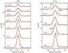 |
Fig. 1 Spectra of the C18O and C17O lines, baseline-subtracted and displaced with a vertical offset between each transition for clarity. The red lines show the Gaussian fits to the spectra. The vertical lines indicate the spectral features attributed to either CH3OH or CH3OCH3. |
3. Observations
The observations were performed between February 28 and October 14, 2010, with the HIFI
instrument on board the Herschel Space Observatory in the double beam
switch mode (180″ chopper
throw). The observed position with Herschel/HIFI toward NGC 6634 I
(α2000 = 17h20m53.32s,
δ2000 = −35°46′58.5″) is located between
the I-SMA1 and I-SMA2 sources (Sect. 2). We employ the same
data reduction process described in Zernickel et al.
(2012); we briefly summarize here the data reduction steps. The data have been
reduced with the HIPE (Herschel Interactive Processing Environment; Ott 2010) pipeline version 5.1. The spectral resolution of the double
sideband (DSB) spectra, which were observed for 3.5 s each, is 1.1 MHz (corresponding to a
velocity resolution ranging from 0.3 km s-1 to 0.6 km s-1). The DSB spectra have been observed with a redundancy
of eight, which allows the deconvolution and isolation of the single sideband (SSB) spectra
(Comito & Schilke 2002). The deconvolved
SSB spectra have been exported to the FITS format for subsequent analysis using the
GILDAS1 package. The half-power beamwidth (HPBW) and
the main beam efficiency (ηmb) for HIFI have been computed as a
function of frequency for each of the observed lines by making linear interpolations from
the values listed in Roelfsema et al. (2012). The
ηmb values are then used to convert the
intensities from the antenna temperature ( ) to the main
beam temperature (Tmb) scale. The spectra shown in this paper
are equally weighted averages of the horizontal and vertical polarizations. In the CHESS
line survey we detect seven C18O lines, five C17O lines, seven HCO+ lines, three H13CO+ lines, and four N2H+ lines. The spatial structure
obtained from SMA (Sect. 2) is unresolved by
Herschel because the beam covers the whole NGC 6334 I region (see Fig. 1
in Zernickel et al. 2012). The SMA observations thus
serve as an auxiliary tool to identify and separate the different components present in the
HIFI spectra.
) to the main
beam temperature (Tmb) scale. The spectra shown in this paper
are equally weighted averages of the horizontal and vertical polarizations. In the CHESS
line survey we detect seven C18O lines, five C17O lines, seven HCO+ lines, three H13CO+ lines, and four N2H+ lines. The spatial structure
obtained from SMA (Sect. 2) is unresolved by
Herschel because the beam covers the whole NGC 6334 I region (see Fig. 1
in Zernickel et al. 2012). The SMA observations thus
serve as an auxiliary tool to identify and separate the different components present in the
HIFI spectra.
4. Results
The spectral line data were analyzed using CLASS, which is part of the GILDAS1 package. The spectra obtained with HIFI towards NGC
6334 I are shown in Figs. 1−3. The
line parameters, derived from a single Gaussian fit to the spectra, are listed in Table
1. The RMS of the integrated intensities
(σI) in Table 1 is computed as 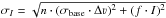 ,
where σbase is the baseline RMS, Δν is the channel width, n is the number of channels
across the line profile that lie above the σbase level of the spectrum,
I = ∫Tmb dV
is the integrated intensity; the factor f, which represents the calibration
uncertainty of the HIFI instrument (Roelfsema et al.
2012), is chosen to be 15%. The rotational spectra of C17O and N2H+ have a hyperfine structure.
However, for the observed lines (Jup ≥ 5) the hyperfine components
are so heavily blended together that, even when determined by a single Gaussian fit, the
line width should not be significantly overestimated (Miettinen et al. 2012).
,
where σbase is the baseline RMS, Δν is the channel width, n is the number of channels
across the line profile that lie above the σbase level of the spectrum,
I = ∫Tmb dV
is the integrated intensity; the factor f, which represents the calibration
uncertainty of the HIFI instrument (Roelfsema et al.
2012), is chosen to be 15%. The rotational spectra of C17O and N2H+ have a hyperfine structure.
However, for the observed lines (Jup ≥ 5) the hyperfine components
are so heavily blended together that, even when determined by a single Gaussian fit, the
line width should not be significantly overestimated (Miettinen et al. 2012).
Line parameters.
The observed molecular lines cover upper level energies in the range 79 K ≤ Eup ≤ 348 K, thus tracing different physical components within the NGC 6334 I region. The detected C18O and HCO+ lines have similar peak intensities, greater than the peak intensities of the N2H+ lines by a factor ranging from ~2 to 10. Also, the average HCO+/H13CO+ line intensity ratio is 18, which is lower than what would be expected in the case of optically thin line emission (12C/ 13C ≈ 75; Langer & Penzias 1990) by a factor of ~4, thus indicating that the HCO+ lines are optically thick. The C18O lines also suffer from optical depth effects with an average C18O/C17O ratio of 2.8, which is lower than the expected value in the case of optically thin line emission (18O/17O ≈ 3.5; Penzias 1981). The C18O and C17O lines have an average value of ⟨Vlsr⟩ = −6.9 ± 0.3 km s-1, and the HCO+ and H13CO+ lines have a value ⟨Vlsr⟩ = −7.4 ± 0.3 km s-1, while the N2H+ lines seem to have a slightly lower value of ⟨Vlsr⟩ = −8.1 ± 0.3 km s-1. These trends are shown in Fig. 4, which is a plot of the velocity and the full-width half-maximum (FWHM) as a function of the upper level energy (Eup) for all the spectral line transitions. Taking into account all of the detected lines, we obtain ⟨Vlsr⟩ = −7.3 ± 0.5 km s-1. As a reference, we include in Fig. 4 the ammonia observations reported by Beuther et al. (2007) associated with the I-SMA1 and I-SMA2 sources.
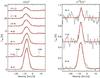 |
Fig. 2 Spectra of the HCO+ and H13CO+ lines, baseline-subtracted and displaced with a vertical offset between each transition for clarity. The red lines show the Gaussian fits to the spectra. The vertical lines indicate the spectral features attributed to CH3OH. |
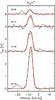 |
Fig. 3 Spectra of the N2H+ lines, baseline-subtracted and displaced with a vertical offset between each transition for clarity. The red lines show the Gaussian fits to the spectra. |
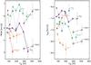 |
Fig. 4 FWHM (left panel) and velocity (right panel) vs. upper level energy Eup, for each of the molecular tracers. The NH3(5,5) and (6,6) observations reported by Beuther et al. (2007) for I-SMA1(triangles) and I-SMA2 (squares) are plotted as reference. |
In terms of the line width, the HCO+ lines are somewhat broader than the C18O and N2H+ lines, and the C17O lines seem to be divided between these two regimes (see Fig. 4). The broadening of the HCO+ lines, when compared to N2H+, is consistent with HCO+ being optically thick, whereas N2H+ is an optically thin tracer. The spread in the C17O line widths can be attributed to line contamination from other molecules, such as methanol (CH3OH) and dimethyl ether (CH3OCH3), present in the C17O spectra. The presence of methanol can also explain some of the spectral features visible in the HCO+ spectra (see the HCO+(7−6) spectrum in Fig. 2, for example). For the HCO+ lines we have an average value of ⟨FWHM⟩ = 6.3 ± 0.4 km s-1, for the C17O lines ⟨FWHM⟩ = 5.5 ± 0.8 km s-1, and for the C18O, N2H+, and H13CO+ lines we have, respectively, ⟨FWHM⟩ = 4.7 ± 0.8 km s-1, 4.5 ± 0.2 km s-1, and 4.6 ± 1.7 km s-1. There is a spread between the H13CO+ lines that produces a larger uncertainty in the average FWHM values, which is probably due to the low signal-to-noise ratio (S/N) in the H13CO+ spectra, particularly in the (7−6) and (8−7) transitions. The H13CO+(6−5) spectrum has the best S/N, and its FWHM is consistent with the line widths obtained from the HCO+ lines. Taking into account all the lines, we obtain ⟨FWHM⟩ = 5.2 ± 1.1 km s-1. The average values obtained from our observations are in agreement, within the uncertainties, with the values obtained from the NH3(5,5) and (6, 6) observations by Beuther et al. (2007). In particular, the observed Vlsr and FWHM values seem to agree more with the parameters of the I-SMA1 source than with those of I-SMA2, but given that only two NH3 transitions are available, and these occur at slightly higher energies compared to the other molecular transitions (see Fig. 4), we cannot reach a definitive conclusion. In addition, the velocities (Vlsr = −7.7 and −7.6 km s-1) and line widths (FWHM = 5.3 and 5.1 km s-1) obtained from the APEX observations (Rolffs et al. 2011) for the C18O(6−5) and (8−7) transitions agree with our results.
In order to search for molecular outflows, we look for the presence of line-wing emission in the spectra and also in their residuals. Since the C18O and HCO+ lines are the brightest transitions, and do not have a hyperfine structure, they are the best candidates to search for outflows. We find that the line-wing emission is very minor (less than 4% of the total integrated line intensity) and is most evident in the C18O(6−5) and HCO+(6−5) transitions, as shown in Fig. 5. In particular, the line-wing emission in the HCO+(6−5) transition is only seen in the red-shifted side of the spectrum. Line-wing emission is also present in the C18O(5−4) and HCO+(8−7) transitions. In the higher-J transitions, either there is no line-wing emission, or it is less evident than in the lower-J transitions.
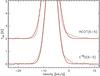 |
Fig. 5 Zoom in on the line-wing emission for the C18O(6−5) and HCO+(6−5) transitions. The red lines show the Gaussian fits to the spectra. |
5. Discussion
5.1. Line profiles and kinematical components
The spectral line profiles (Figs. 1−3) for the lower energy transitions of C18O, C17O, HCO+, and N2H+ are asymmetric, with the redshifted side of the profile being stronger than the blueshifted side. This red asymmetry is consistent with emission from optically thick lines from expanding gas. We note that the asymmetry is not seen in the optically thin H13CO+ spectra, and is much less evident in the higher energy transitions of the other molecules. Although it may be just a fortuitous case, the simultaneous presence of the asymmetry in the optically thick lines and absence in the optically thin lines is evidence of the presence of an expanding motion of the emitting gas (Mardones et al. 1997).
In the following, we present a quantitative analysis of the line profiles in support of the expanding gas hypothesis. As mentioned above, in most cases, a single Gaussian does not fit the observations properly. We attempt to improve the analysis by using a double Gaussian fit in order to decompose the spectra into two kinematical components, which can be justified by the presence of two different velocity components in the line profile. Based on our analysis, and also on the results from previous observations toward NGC 6334 I, we initially assign a velocity of −6.6 km s-1 to the emission from the envelope, and a velocity of −9.8 km s-1 to the emission from the core. However, this fit is not unique, as demonstrated by an a posteriori analysis of the spectra, in which we used the results from our radiative transfer analysis (Sect. 5.2) as input parameters for a two-component Gaussian model. The spectra suggest the presence of a velocity gradient, which is also consistent with our hypothesis of an expanding envelope, as discussed in Sect. 5.3.
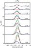 |
Fig. 6 Example of the C18O spectra, overlaid with the double Gaussian profile derived from the results of the LVG analysis. The red, blue, and green lines show, respectively, the Gaussian profiles for the outer and inner envelope emission, and the sum of the two components. |
As an example, we show in Fig. 6 the double Gaussian profile for the C18O spectra. We assign, for the outer and inner envelope emission respectively, velocities of −6.0 km s-1 and −7.5 km s-1, line widths of 4.0 km s-1 and 4.7 km s-1; the line intensity ratios between the two components are the ones derived from the radiative transfer analysis. Since neither the single Gaussian fit nor the two-component Gaussian model can reproduce the line profiles accurately for all molecular transitions, we alternatively derive the integrated line intensities by computing the area obtained by summing all channels across the line profile and compare the results with the corresponding values obtained from the single Gaussian fit. Given that for the radiative transfer analysis we are mainly interested in the total emission from the spectra, and that the difference between the integrated intensities obtained by the two aforementioned methods ranges from 0−4% (with a median value of 1%), we conclude that the results from the single Gaussian profile are appropriate to perform the radiative transfer analysis.
5.2. Non-LTE analysis
With the results obtained from the Gaussian fits (Table 1), and using a non-LTE LVG radiative transfer code (Ceccarelli et al. 2003), we model the spectral line emission of the observed transitions in order to obtain estimates of the temperature; H2 density; size; and CO, HCO+, and N2H+ column density in NGC 6334 I. We achieve this by comparing the observations with the LVG predictions and obtaining a best-fit model by χ2 optimization. The optimization is done by first finding the best reduced χ2 value for each input value of column density, minimizing it with respect to the other model parameters (i.e., temperature, molecular hydrogen density, and source size). Afterwards, the minimum χ2 obtained from the set of column densities corresponds to the model that best fits our results. The uncertainties of the best-fit model are estimated by obtaining the adjustable parameter ranges within the 1σ confidence level, and using the appropriate number of degrees of freedom for each set of molecular transitions. The non-LTE LVG code makes use of the collisional coefficients calculated by Flower (1999) for HCO+ and N2H+. We note that Flower (1999) reports calculations of the HCO+ − para-H2 system for the first 21 energy levels in the temperature range 5 ≤ T ≤ 390 K. In our analysis, we use the same coefficients for N2H+ and assume an ortho- to para-H2 ratio equal to 0.01, meaning that nearly all H2 molecules are in the para state. The collisional coefficients have been retrieved from the BASECOL database2 (Dubernet et al. 2013).
Results of LVG analysis.
The rotational transitions of HCO+, H13CO+, N2H+, and the CO isotopologues all have similar upper level energies and, with the exception of the CO isotopologues, they all have similar critical densities as well. All of these transitions are thus likely to probe the same volume of gas within the observed region. Therefore, we aim to find the model that best fits all the molecular transitions simultaneously. To achieve this, we first fit the C18O and C17O spectral line emission by χ2 optimization. Both isotopologues are fitted simultaneously, thus imposing stronger constraints on the model parameters. In practice, a one-component model cannot fit the observations properly, indicating that there are indeed two physical components with different physical conditions along the line of sight (Sect. 5.1). We therefore fit the observations with a two-component model: a posteriori, the two components correspond to two regions of the envelope (see Sect. 5.3). Afterwards, the HCO+ and H13CO+ spectral line emission are fitted simultaneously, using the H2 density, temperature, and source size parameters derived from the CO model as input values and adjusting the molecular column density in order to obtain the best fit. This last step is repeated for the N2H+ spectral line emission, so in the end all molecular transitions are fitted with a two-component LVG model, in which the C18O, HCO+, and N2H+ column densities are the only varying parameters. The results from this method are presented in Table 2 and Fig. 7.
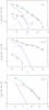 |
Fig. 7 Plots of integrated intensity vs. Jup (from top to bottom) for the C18O (red stars) and C17O (red squares), HCO+ (stars) and H13CO+ (squares), and N2H+ (stars) spectral line emission, obtained from the LVG model. The blue and pink lines represent, respectively, the theoretical model for the outer and inner envelope components, and the green lines represent the sum of the two components. The solid lines represent the model results for C18O, HCO+, and N2H+, while the dashed lines represent the model results for C17O and H13CO+. |
We note that a small variation in the H2 density, temperature, and source size values obtained from the CO model is necessary to best fit all molecular transitions simultaneously, thus making the radiative transfer modeling an iterative process. However, the variation between the integrated intensities of the χ2 optimized model and the final best-fit model is less than the uncertainties listed in the last column in Table 1. We also note that the C17O(8−7) transition is excluded from the LVG analysis because it is contaminated by CH3OCH3 emission (see Fig. 1). Finally, given the small number of detected N2H+ transitions, a one-component model could have been used to fit these observations, but we choose to consistently use the two-component model that is needed to explain the other molecular species considered in this work.
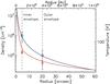 |
Fig. 8 Radial profiles of the density (blue line) and temperature (red line) toward NGC 6334 I from R11. The vertical lines indicate, respectively, the radius of the inner and outer regions obtained from our LVG analysis. The density (blue squares) and temperature (red triangles) values obtained for each component are overlaid on the plot. |
5.3. Origin of the emission: the expanding envelope
The radial profiles of density and temperature for NGC 6334 I, obtained by using the specific parameters from the analysis of R11 (Sect. 2), are presented in Fig. 8. The parameters obtained from our LVG analysis (Table 2) are overlaid on the profiles to compare the two methods. The outer and inner envelope angular radii obtained from the LVG analysis, which are also shown in Fig. 8, correspond to a density and temperature of ~9 × 104 cm-3 and 38 K for the outer region, and ~9× 105 cm-3 and 72 K for the inner region. The results from our analysis are thus remarkably consistent with the radial structure modeled by R11 for NGC 6334 I. As already mentioned in Sect. 2, the interferometric observations from SMA (Hunter et al. 2006) revealed that the hot core of NGC 6334 I is composed of various compact condensations within an angular size of ≈10″. Although the Herschel/HIFI observations cannot resolve the spatial structure of the hot core, the high level of agreement between the results from our LVG analysis and the results from the radial structure of R11 lead us to the conclusion that our spectral lines are dominated by the emission from the envelope of NGC 6334 I. We will therefore refer to the two components as the outer and inner envelope. In addition, as mentioned in Sect. 5.1, the red asymmetry displayed in the spectra is consistent with expanding gas, and the Gaussian fits to the line profiles suggest a velocity gradient in the envelope. The LVG analysis shows that there are two major physical components that we can identify with two kinematical components, with velocities of −6.0 km s-1 and −7.5 km s-1. We emphasize that these two velocity components are probably the two extremes of a gradual change in velocity through the envelope and we do not claim that our analysis fully reproduces the observed profiles. It makes, however, the important point that there is an expansion movement in the envelope with a gradient between the inner and outer envelope, namely on a scale of about 2.6 × 10⁴ AU, of about 1.5 km s-1. The results are summarized in Fig. 9, which is a representation of the expanding envelope. A full radiative transfer modeling of the line profiles as well as additional higher resolution spectral line observations to properly constrain the model parameters would be needed to determine the properties of the velocity gradient in the envelope, but this kind of analysis is beyond the scope of the present work.
Previous studies of giant molecular clouds and HII regions (e.g., Bally & Scoville 1980; Krumholz & Matzner 2009; Lopez et al. 2011) suggest that, given the expansion velocity and the radial distance at which the expansion would be taking place, thermal pressure from hot ionized gas should dominate the envelope expansion in NGC 6334 I. To give an estimate, using Eq. (9) in Garcia-Segura & Franco (1996) we find that the flux of ionizing photons produced by the UCHII region associated with NGC 6334 I (de Pree et al. 1995) can exert a thermal pressure, Pt/k, on the surrounding envelope of 1.6 × 109 cm-3 K. Using the results from our analysis, and the right-hand side of Eq. (2) in Olmi & Cesaroni (1999), we estimate that the ambient pressure, Pa/k, exerted by the envelope is between 108 cm-3 K and 109 cm-3 K. Therefore, it is energetically possible to have an envelope expansion in NGC 6334 I. The derived physical parameters for the expanding envelope are discussed further in the following section.
We note that our conclusion of an expanding envelope toward NGC 6334 I is subject to some caveats. First, the analysis of the SMA data by Zernickel et al. (2012), as well as the ATCA observations by Beuther et al. (2007) (Sect. 2), indicate a velocity difference between the I-SMA1 and I-SMA2 cores. The emission from these two sources could potentially introduce line asymmetries such as the ones observed in the HIFI spectra. Alternatively, the observed line profiles could be caused by emission from gas that is entrained in an outflow near or along the line of sight. However, we consider both these scenarios unlikely for the following reasons:
-
1.
The HIFI observations also sample gas at spatial scales that have been filtered out in the SMA maps. Thus, the velocity difference we measure may have a different origin compared to that between I-SMA1 and I-SMA2.
-
2.
The abundance of molecular ions is expected to be lower toward the very central region of NGC 6334 I because of the lower CR ionization in such a dense region. Our HCO+ and N2H+ observations are thus more likely to probe a much larger volume of gas compared to that of the interferometric observations.
-
3.
The HCO+ and N2H+ emitting sizes (Table 2) are larger than those measured for the hot cores, while they are consistent with emission from a larger scale, such as that from the envelope.
-
4.
R11 found infall signatures in HCN high-excitation lines, while our HCO+ line profiles show no signs of infall, which suggests that our spectra are mostly sensitive to less dense gas.
-
5.
The direction of the bipolar outflow in NGC 6334 I is in the northeast-southwest direction (PA ~ 46°), as first reported by CO and SiO observations (Bachiller & Cernicharo 1990) and later confirmed by subsequent observations (e.g., Kraemer & Jackson 1995; Leurini et al. 2006; Beuther et al. 2008). In particular, Leurini et al. (2006) reported that the small overlap between the outflow lobes indicates that the inclination angle of the bipolar outflow is closer to 90° than to 0°. It is thus unlikely that the outflow is responsible for the asymmetries observed in the line profiles, as it is far enough from the line of sight. We cannot exclude the possibility of another unresolved outflow along the line of sight, but this is not yet supported by any available data.
5.4. Ionization structure of the envelope
5.4.1. Column densities and molecular abundances
Using the results from the LVG analysis we can derive estimates of the H2 column density, as well as the relative abundances between the various molecular species. With the column densities of HCO+ and N2H+ listed in Table 2 we obtain an [HCO+]/[N2H+] abundance ratio of 6 and 23 for the outer and inner envelope components, respectively. We derive the CO column densities using an abundance ratio of [CO]/[C18O] = 500 (Wilson & Rood 1994), and from the H2 densities and the linear size of the inner and outer envelope we compute the H2 column densities. Afterwards, we obtain the relative abundances of HCO+ and N2H+ with respect to H2 as well as the [CO]/[H2] abundance ratios. These results are listed in Table 3 where, with the exception of the [HCO+]/[N2H+] ratio, the uncertainties of the derived parameters are estimated using the standard method of error propagation. For the [HCO+]/[N2H+] abundance ratio, the uncertainties are instead determined by analyzing the variation in the ratio of the resulting HCO+ and N2H+ column densities for all LVG solutions within the 1σ confidence level (see Sect. 5.2). During this procedure the two sets of [HCO+]/[N2H+] ratios (one for the outer and one for the inner envelope) used to determine the uncertainties are computed from pairs of solutions with equal (within a 5% tolerance) model parameters (i.e., H2 density, temperature, and source size). We choose to apply this method instead of the standard error propagation because the latter would artificially increase the resulting uncertainties because the uncertainties of the [HCO+]/[H2] and [N2H+]/[H2] ratios must take into account the variation of H2 density, gas temperature, and source size within the 1σ confidence level for the LVG model.
As a comparison, we also list in Table 3 the H2 column densities computed using the radial density profile from R11 and the same method described above, which are consistent with our results. Although there is no clear trend in the molecular abundances when the uncertainties are taken into account, if we consider the [HCO+]/[N2H+] abundance ratios we find that it is definitively different in the inner envelope when compared to that in the outer envelope.
For the computation of the CO column densities we assume, as is common practice, that the [CO]/[C18O] ratio equals the [16O]/[18O] ratio. This oxygen isotopic ratio has been estimated for the ISM by Smith et al. (2009) as a function of the source distance from the Galactic center. Using Eq. (4) in Smith et al. (2009) with a Galactocentric distance of 6.8 kpc for NGC 6334 (Kraemer et al. 1998, 2000) we obtain a [16O]/[18O] ratio of 488 ± 68 for NGC 6334 I. The difference with respect to the value of 500 adopted above for the [16O]/[18O] ratio is less than 3%, and therefore does not affect our results for the relative abundances.
Derived parameters.
For the [CO]/[H2] abundance ratio, we obtain values of 3 × 10⁻⁴ and 5 × 10⁻⁴ for the outer and inner envelope, which are higher than the standard dense cloud value of 10-4 (Burgh et al. 2007, and references therein). These abundance ratios are obtained using H2 column densities of 1023 and 2 × 1023 cm-2 for the outer and inner envelope respectively, as listed in Table 3. There are two alternative methods of computing the H2 column density in addition to the one previously described.
The first alternative method is to use the derived CO column density and the
[CO]/[H2] standard dense cloud value to compute the
H2 column
density. Using this method we obtain higher H2 column densities by a factor of 3 and 5 for the outer
and inner envelope of NGC 6334 I. The second alternative method is to assume the source
has a spherical symmetry and a radial density profile of the form  (1)where n0 and
R are,
respectively, the H2 density and envelope radius for the outer and inner
components. The H2 column densities are then computed by integrating this
density profile along the line of sight, after a convolution with a 2D Gaussian
corresponding to the HIFI beam. Using this method, we obtain H2 column densities that are
lower by a factor of 1.7 and 2, and [CO]/[H2] abundance ratios of 5 × 10⁻⁴ and 10-3 for the outer and inner
envelope. The results from this method are within the uncertainties of the values listed
in Table 3. A more detailed radiative transfer
analysis that also takes into account the non-spherical envelope structure would be
needed to better understand the variations in the column density and [CO]/[H2] abundance ratio, but this
analysis is beyond the scope of the present work.
(1)where n0 and
R are,
respectively, the H2 density and envelope radius for the outer and inner
components. The H2 column densities are then computed by integrating this
density profile along the line of sight, after a convolution with a 2D Gaussian
corresponding to the HIFI beam. Using this method, we obtain H2 column densities that are
lower by a factor of 1.7 and 2, and [CO]/[H2] abundance ratios of 5 × 10⁻⁴ and 10-3 for the outer and inner
envelope. The results from this method are within the uncertainties of the values listed
in Table 3. A more detailed radiative transfer
analysis that also takes into account the non-spherical envelope structure would be
needed to better understand the variations in the column density and [CO]/[H2] abundance ratio, but this
analysis is beyond the scope of the present work.
5.4.2. Chemical modeling
We model the chemical evolution of the source using the gas-phase reaction network from the KInetic Database for Astrochemistry (KIDA) in conjunction with the Nahoon code (Wakelam et al. 2012). The KIDA network contains over 6000 unique chemical reactions involving almost 500 different species and a total of 6467 rate coefficients. The Nahoon code uses this database to compute the time-dependent gas-phase chemistry at a fixed temperature (between 10−300 K), density, and CR ionization rate. A set of reactions involving grains that are not included in KIDA, such as the formation of H2 on grains, are also included in Nahoon (see Table 3 in Wakelam et al. 2012 for a description). The formation of HCO+ and N2H+ in dense regions (e.g., Turner 1995; Bergin et al. 1997) is dominated by the CR ionization rate. Consequently, the abundances of these molecular ions, as well as their abundance ratio, provide us with an ideal tool to estimate the CR ionization rate toward the envelope of NGC 6334 I. By running a 10 × 10 grid of Nahoon models, sampled logarithmically in a range of H2 densities and CR ionization rates (ζH2), we compute the expected [HCO+]/[N2H+] abundance ratios for the two temperature components. In these models, the initial abundances are taken from Table 2 in Wakelam et al. (2010) where all species are in the atomic form except for molecular hydrogen, and the final abundances are computed for steady state (107 yr). Through the comparison of the model results with the H2 densities and [HCO+]/[N2H+] abundance ratios derived from the LVG analysis, we then obtain an estimate for ζH2 toward NGC 6334 I.
Using this method we find, for the outer and inner envelope components respectively, CR ionization rates of 2.0 × 10⁻¹⁶ s-1 and 8.5 × 10⁻¹⁷ s-1, which are both higher than the standard CR ionization rate in molecular clouds of ζH2 ≈ 10-17 s-1 (Padovani et al. 2009, and references therein). We note that the values of ζH2, and also the H2 column densities, obtained for NGC 6334 I are similar to previous values obtained by van der Tak & van Dishoeck (2000) and Doty et al. (2002) toward the envelopes surrounding massive protostellar sources. In Fig. 10 we present the computed [HCO+]/[N2H+] abundance ratio as a function of the CR ionization rate for the outer and inner envelope components, in which the H2 densities and temperatures obtained from the LVG analysis have been used as input parameters for the Nahoon model. Overlaid are the ranges of abundance ratios and CR ionization rates obtained for each component when the [HCO+]/[N2H+] ratio is varied by the uncertainties listed in Table 3. There seems to be a trend for the CR ionization rate in the envelope to increase outward, but because of our uncertainties (see Fig. 10) this conclusion remains uncertain.
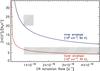 |
Fig. 10 [HCO+]/[N2H+] abundance ratio as a function of the CR ionization rate computed for the inner (blue line) and outer (red line) envelope components using the Nahoon code. The shaded areas represent the results obtained within the uncertainties listed in Table 3. The ζH2 values in the upper-left and lower-right corners of the shaded areas correspond to the maximum and minimum values of the [HCO+]/[N2H+] ratio, respectively (see text for discussion). |
The tentative trend for the CR ionization rate would suggest that the main source of
ionization originates outside of NGC 6334 I. It has already been mentioned that the
ionization in dense regions, like the envelope of NGC 6334 I, is dominated by CRs. But
X-ray emission from young massive stars in the surrounding molecular cloud could also
contribute as a source of ionization. X-ray emission in the NGC 6334 giant molecular
cloud has been revealed through observations with the Advanced Satellite for
Cosmology and Astrophysics (ASCA; Sekimoto
et al. 2000) and the Chandra X-Ray Observatory (Ezoe et al. 2006) in the energy range of
0.5−10 keV. The X-ray
emission is mainly associated with young massive stars embedded in the five far-infrared
(FIR) regions denoted NGC 6334 I−V. Therefore, the nearest sources of X-rays should be cores
II−V in NGC 6334 and the
interior of NGC 6334 I itself. From the ASCA observations, Sekimoto et al. (2000) obtained X-ray luminosities (LX) and
hydrogen column densities (NH) for each of the five cores, and
then computed the radius (rX) inside which the X-ray ionization
rate (ζX) is comparable to the standard value
for the CR ionization rate using the equation given by Maloney et al. (1996): 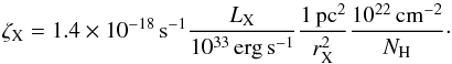 (2)With X-ray
luminosities of ~1033 erg s-1 and column densities of ~1022 cm-2 for each of the five cores,
and assuming ζX = 10-17 s-1, Sekimoto and co-authors
determined that the X-ray ionization rate is comparable to that by CRs within a radius
of ~0.3 pc from each core.
This distance is much smaller than the distance between cores II−V and core I, and therefore there should
be no significant ionization in NGC 6334 I due to external X-ray sources. The authors
obtained LX = 0.66 × 1033 erg s-1 and NH = 2.0 × 10²²
cm-2 for the
X-ray emission from the interior of NGC 6334 I. By using equation (2) with our ζH2
values from Table 3, we obtain that X-ray
ionization for the outer envelope (r = 0.16 pc) is comparable to CR ionization up to
a radius of 0.05 pc. The ionization in the outer envelope should thus be dominated by
CRs. However for the inner envelope (r = 0.04 pc) X-ray ionization is comparable to
that by CRs up to a radius of 0.07 pc. Therefore the CR ionization rate value for the
inner envelope should be treated as an upper limit due to any additional contribution
from X-ray emission.
(2)With X-ray
luminosities of ~1033 erg s-1 and column densities of ~1022 cm-2 for each of the five cores,
and assuming ζX = 10-17 s-1, Sekimoto and co-authors
determined that the X-ray ionization rate is comparable to that by CRs within a radius
of ~0.3 pc from each core.
This distance is much smaller than the distance between cores II−V and core I, and therefore there should
be no significant ionization in NGC 6334 I due to external X-ray sources. The authors
obtained LX = 0.66 × 1033 erg s-1 and NH = 2.0 × 10²²
cm-2 for the
X-ray emission from the interior of NGC 6334 I. By using equation (2) with our ζH2
values from Table 3, we obtain that X-ray
ionization for the outer envelope (r = 0.16 pc) is comparable to CR ionization up to
a radius of 0.05 pc. The ionization in the outer envelope should thus be dominated by
CRs. However for the inner envelope (r = 0.04 pc) X-ray ionization is comparable to
that by CRs up to a radius of 0.07 pc. Therefore the CR ionization rate value for the
inner envelope should be treated as an upper limit due to any additional contribution
from X-ray emission.
Finally, we compute the theoretical value of the CR ionization rate as a function of the column density of traversed matter for NGC 6334 I using the model from Padovani et al. (2009). The model provides four possible profiles of the CR ionization rate depending on how the energy distribution of CR particles incident on the source is defined, and includes a detailed treatment of CR propagation that takes into account the decrease of the ionization rate as the CRs penetrate the cloud. Using the N[H2] column densities in Table 3 we find that the M02+E00 model3 of Padovani et al. (2009) provides the profile that best agrees with our results, and from it we obtain CR ionization rates of 1.4 × 10⁻¹⁶ s-1 and 9.5 × 10⁻¹⁷ s-1 for the outer and inner envelope components, respectively. The agreement, within the uncertainties, between the results from the KIDA/Nahoon model and the model from Padovani et al. (2009) suggests that interstellar CRs alone are capable of producing the ionization rates obtained for NGC 6334 I and, therefore, additional sources of ionization are not required in order to explain our results.
6. Summary and conclusions
We presented high-resolution spectral line observations of the high-mass star-forming region NGC 6334 I obtained with the HIFI instrument on board Herschel. In total, five molecular species were analyzed through several rotational transitions with Jup ≥ 5. The results of our study can be summarized as follows:
-
1.
We detect bright emission from the HCO+ and N2H+ molecular ions, which allows us to constrain the ionization in the warm and dense regions of NGC 6334 I.
-
2.
Optically thick HCO+ and N2H+ lines display profiles with a redshifted asymmetry, while optically thin H13CO+ lines have a Gaussian profile peaked at the absorption dip of the optically thick lines. This is consistent with an expanding gas.
-
3.
A non-LTE LVG radiative transfer analysis of the integrated line intensities shows the presence of two major physical components whose temperatures and densities are consistent with those previously derived from the radial structure of the envelope of NGC 6334 I.
-
4.
We find evidence supporting the scenario in which the envelope surrounding the hot core of NGC 6334 I is expanding and thermal pressure from hot ionized gas is able to provide the driving force required for the envelope expansion.
-
5.
We find a tentative trend for the CR ionization rate in the envelope to increase outward, which would suggest that the main source of ionization lies outside NGC 6334 I. The ionization in the outer envelope is probably dominated by CRs, but there could be an additional contribution to the ionization in the inner envelope from X-ray emission originating in the interior of NGC 6334 I.
-
6.
The values obtained for the CR ionization rate are consistent, within the errors, with the model from Padovani et al. (2009) that computes the CR ionization rate through a detailed treatment of CR propagation in molecular clouds, and they are also similar to previous values obtained toward the envelopes surrounding massive protostellar sources.
In this model, the energy distribution of CR particles is defined using the estimates of Moskalenko et al. (2002) and Strong et al. (2000). See Padovani et al. (2009) for a detailed description.
Acknowledgments
HIFI has been designed and built by a consortium of institutes and university departments from across Europe, Canada and the United States under the leadership of SRON Netherlands Institute for Space Research, Groningen, The Netherlands, and with major contributions from Germany, France and the US. Consortium members are: Canada: CSA, U.Waterloo; France: CESR, LAB, LERMA, IRAM; Germany: KOSMA, MPIfR, MPS; Ireland: NUI Maynooth; Italy: ASI, IFSI-INAF, Osservatorio Astrofisico di Arcetri-INAF; Netherlands: SRON, TUD; Poland: CAMK, CBK; Spain: Observatorio Astronómico Nacional (IGN), Centro de Astrobiología (CSIC-INTA); Sweden: Chalmers University of Technology − MC2, RSS & GARD; Onsala Space Observatory; Swedish National Space Board, Stockholm University − Stockholm Observatory; Switzerland: ETH Zurich, FHNW; USA: Caltech, JPL, NHSC. Support for this work was provided by NASA through an award issued by JPL/Caltech. J.M.O. acknowledges the support of NASA, through the PR NASA Space Grant Doctoral Fellowship, and from the Institut de Planétologie et d’Astrophysique de Grenoble (IPAG). C.C. acknowledges the financial support from the French Agence Nationale pour la Recherche (ANR) (project FORCOMS, contract ANR-08-BLAN-0225) and the French spatial agency CNES. The authors wish to thank Marco Padovani for providing the models for computing the CR ionization rate, as well as the anonymous referee and Ana López-Sepulcre, whose comments much contributed to improve this work.
References
- Bachiller, R., & Cernicharo, J. 1990, A&A, 239, 276 [NASA ADS] [Google Scholar]
- Balbus, S. A., & Hawley, J. F. 1998, Rev. Mod. Phys., 70, 1 [Google Scholar]
- Bally, J., & Scoville, N. Z. 1980, ApJ, 239, 121 [NASA ADS] [CrossRef] [Google Scholar]
- Bergin, E. A., Goldsmith, P. F., Snell, R. L., & Langer, W. D. 1997, ApJ, 482, 285 [NASA ADS] [CrossRef] [Google Scholar]
- Beuther, H., Thorwirth, S., Zhang, Q., et al. 2005, ApJ, 627, 834 [NASA ADS] [CrossRef] [Google Scholar]
- Beuther, H., Walsh, A. J., Thorwirth, S., et al. 2007, A&A, 466, 989 [NASA ADS] [CrossRef] [EDP Sciences] [Google Scholar]
- Beuther, H., Walsh, A. J., Thorwirth, S., et al. 2008, A&A, 481, 169 [NASA ADS] [CrossRef] [EDP Sciences] [Google Scholar]
- Brooks, K. J., & Whiteoak, J. B. 2001, MNRAS, 320, 465 [NASA ADS] [CrossRef] [Google Scholar]
- Burgh, E. B., France, K., & McCandliss, S. R. 2007, ApJ, 658, 446 [NASA ADS] [CrossRef] [Google Scholar]
- Ceccarelli, C., Maret, S., Tielens, A. G. G. M., Castets, A., & Caux, E. 2003, A&A, 410, 587 [NASA ADS] [CrossRef] [EDP Sciences] [Google Scholar]
- Ceccarelli, C., Bacmann, A., Boogert, A., et al. 2010, A&A, 521, L22 [NASA ADS] [CrossRef] [EDP Sciences] [Google Scholar]
- Ceccarelli, C., Hily-Blant, P., Montmerle, T., et al. 2011, ApJ, 740, L4 [Google Scholar]
- Cesaroni, R. 2005, in Massive Star Birth: A Crossroads of Astrophysics, eds. R. Cesaroni, M. Felli, E. Churchwell, & M. Walmsley, IAU Symp., 227, 59 [Google Scholar]
- Codella, C., Lefloch, B., Ceccarelli, C., et al. 2010, A&A, 518, L112 [NASA ADS] [CrossRef] [EDP Sciences] [Google Scholar]
- Comito, C., & Schilke, P. 2002, A&A, 395, 357 [NASA ADS] [CrossRef] [EDP Sciences] [Google Scholar]
- de Pree, C. G., Rodriguez, L. F., Dickel, H. R., & Goss, W. M. 1995, ApJ, 447, 220 [NASA ADS] [CrossRef] [Google Scholar]
- Doty, S. D., van Dishoeck, E. F., van der Tak, F. F. S., & Boonman, A. M. S. 2002, A&A, 389, 446 [NASA ADS] [CrossRef] [EDP Sciences] [Google Scholar]
- Dubernet, M.-L., Alexander, M. H., Ba, Y. A., et al. 2013, A&A, 553, A50 [NASA ADS] [CrossRef] [EDP Sciences] [Google Scholar]
- Emprechtinger, M., Lis, D. C., Bell, T., et al. 2010, A&A, 521, L28 [NASA ADS] [CrossRef] [EDP Sciences] [Google Scholar]
- Emprechtinger, M., Lis, D. C., Rolffs, R., et al. 2013, ApJ, 765, 61 [NASA ADS] [CrossRef] [Google Scholar]
- Ezoe, Y., Kokubun, M., Makishima, K., Sekimoto, Y., & Matsuzaki, K. 2006, ApJ, 638, 860 [NASA ADS] [CrossRef] [Google Scholar]
- Flower, D. R. 1999, MNRAS, 305, 651 [NASA ADS] [CrossRef] [Google Scholar]
- Gammie, C. F. 1996, ApJ, 457, 355 [NASA ADS] [CrossRef] [Google Scholar]
- Garcia-Segura, G., & Franco, J. 1996, ApJ, 469, 171 [NASA ADS] [CrossRef] [Google Scholar]
- Hunter, T. R., Brogan, C. L., Megeath, S. T., et al. 2006, ApJ, 649, 888 [NASA ADS] [CrossRef] [Google Scholar]
- Kama, M., López-Sepulcre, A., Dominik, C., et al. 2013, A&A, 556, A57 [Google Scholar]
- Kraemer, K. E., & Jackson, J. M. 1995, ApJ, 439, L9 [NASA ADS] [CrossRef] [Google Scholar]
- Kraemer, K. E., Jackson, J. M., & Lane, A. P. 1998, ApJ, 503, 785 [NASA ADS] [CrossRef] [Google Scholar]
- Kraemer, K. E., Jackson, J. M., Lane, A. P., & Paglione, T. A. D. 2000, ApJ, 542, 946 [NASA ADS] [CrossRef] [Google Scholar]
- Krumholz, M. R., & Matzner, C. D. 2009, ApJ, 703, 1352 [NASA ADS] [CrossRef] [Google Scholar]
- Langer, W. D., & Penzias, A. A. 1990, ApJ, 357, 477 [NASA ADS] [CrossRef] [Google Scholar]
- Leurini, S., Schilke, P., Parise, B., et al. 2006, A&A, 454, L83 [NASA ADS] [CrossRef] [EDP Sciences] [Google Scholar]
- Lis, D. C., Pearson, J. C., Neufeld, D. A., et al. 2010, A&A, 521, L9 [NASA ADS] [CrossRef] [EDP Sciences] [Google Scholar]
- Lopez, L. A., Krumholz, M. R., Bolatto, A. D., Prochaska, J. X., & Ramirez-Ruiz, E. 2011, ApJ, 731, 91 [NASA ADS] [CrossRef] [Google Scholar]
- Maloney, P. R., Hollenbach, D. J., & Tielens, A. G. G. M. 1996, ApJ, 466, 561 [NASA ADS] [CrossRef] [Google Scholar]
- Mardones, D., Myers, P. C., Tafalla, M., et al. 1997, ApJ, 489, 719 [NASA ADS] [CrossRef] [Google Scholar]
- Miettinen, O., Harju, J., Haikala, L. K., & Juvela, M. 2012, A&A, 538, A137 [NASA ADS] [CrossRef] [EDP Sciences] [Google Scholar]
- Migenes, V., Horiuchi, S., Slysh, V. I., et al. 1999, ApJS, 123, 487 [NASA ADS] [CrossRef] [Google Scholar]
- Moskalenko, I. V., Strong, A. W., Ormes, J. F., & Potgieter, M. S. 2002, ApJ, 565, 280 [Google Scholar]
- Neckel, T. 1978, A&A, 69, 51 [NASA ADS] [Google Scholar]
- Olmi, L., & Cesaroni, R. 1999, A&A, 352, 266 [NASA ADS] [Google Scholar]
- Ossenkopf, V., Müller, H. S. P., Lis, D. C., et al. 2010, A&A, 518, L111 [NASA ADS] [CrossRef] [EDP Sciences] [Google Scholar]
- Ott, S. 2010, in Astronomical Data Analysis Software and Systems XIX, eds. Y. Mizumoto, K.-I. Morita, & M. Ohishi, ASP Conf. Ser., 434, 139 [Google Scholar]
- Padovani, M., Galli, D., & Glassgold, A. E. 2009, A&A, 501, 619 [NASA ADS] [CrossRef] [EDP Sciences] [Google Scholar]
- Padovani, M., Galli, D., & Glassgold, A. E. 2013, A&A, 549, C3 [NASA ADS] [CrossRef] [EDP Sciences] [Google Scholar]
- Penzias, A. A. 1981, ApJ, 249, 518 [NASA ADS] [CrossRef] [Google Scholar]
- Rivera-Ingraham, A., Martin, P. G., Polychroni, D., et al. 2013, ApJ, 766, 85 [NASA ADS] [CrossRef] [Google Scholar]
- Roelfsema, P. R., Helmich, F. P., Teyssier, D., et al. 2012, A&A, 537, A17 [NASA ADS] [CrossRef] [EDP Sciences] [Google Scholar]
- Rolffs, R., Schilke, P., Wyrowski, F., et al. 2011, A&A, 527, A68 (R11) [NASA ADS] [CrossRef] [EDP Sciences] [Google Scholar]
- Sandell, G. 2000, A&A, 358, 242 [NASA ADS] [Google Scholar]
- Sekimoto, Y., Matsuzaki, K., Kamae, T., et al. 2000, PASJ, 52, L31 [NASA ADS] [Google Scholar]
- Smith, R. L., Pontoppidan, K. M., Young, E. D., Morris, M. R., & van Dishoeck, E. F. 2009, ApJ, 701, 163 [NASA ADS] [CrossRef] [Google Scholar]
- Strong, A. W., Moskalenko, I. V., & Reimer, O. 2000, ApJ, 537, 763 [Google Scholar]
- Turner, B. E. 1995, ApJ, 449, 635 [NASA ADS] [CrossRef] [Google Scholar]
- van der Tak, F. F. S., & van Dishoeck, E. F. 2000, A&A, 358, L79 [NASA ADS] [Google Scholar]
- van der Wiel, M. H. D., van der Tak, F. F. S., Lis, D. C., et al. 2010, A&A, 521, L43 [Google Scholar]
- Wakelam, V., Herbst, E., Le Bourlot, J., et al. 2010, A&A, 517, A21 [NASA ADS] [CrossRef] [EDP Sciences] [Google Scholar]
- Wakelam, V., Herbst, E., Loison, J.-C., et al. 2012, ApJS, 199, 21 [NASA ADS] [CrossRef] [Google Scholar]
- Walsh, A. J., Burton, M. G., Hyland, A. R., & Robinson, G. 1998, MNRAS, 301, 640 [NASA ADS] [CrossRef] [Google Scholar]
- Walsh, A. J., Longmore, S. N., Thorwirth, S., Urquhart, J. S., & Purcell, C. R. 2007, MNRAS, 382, L35 [NASA ADS] [Google Scholar]
- Wilson, T. L., & Rood, R. 1994, ARA&A, 32, 191 [NASA ADS] [CrossRef] [Google Scholar]
- Zernickel, A., Schilke, P., Schmiedeke, A., et al. 2012, A&A, 546, A87 [NASA ADS] [CrossRef] [EDP Sciences] [Google Scholar]
- Zinnecker, H., & Yorke, H. W. 2007, ARA&A, 45, 481 [NASA ADS] [CrossRef] [Google Scholar]
All Tables
All Figures
|
Fig. 1 Spectra of the C18O and C17O lines, baseline-subtracted and displaced with a vertical offset between each transition for clarity. The red lines show the Gaussian fits to the spectra. The vertical lines indicate the spectral features attributed to either CH3OH or CH3OCH3. |
| In the text | |
|
Fig. 2 Spectra of the HCO+ and H13CO+ lines, baseline-subtracted and displaced with a vertical offset between each transition for clarity. The red lines show the Gaussian fits to the spectra. The vertical lines indicate the spectral features attributed to CH3OH. |
| In the text | |
|
Fig. 3 Spectra of the N2H+ lines, baseline-subtracted and displaced with a vertical offset between each transition for clarity. The red lines show the Gaussian fits to the spectra. |
| In the text | |
|
Fig. 4 FWHM (left panel) and velocity (right panel) vs. upper level energy Eup, for each of the molecular tracers. The NH3(5,5) and (6,6) observations reported by Beuther et al. (2007) for I-SMA1(triangles) and I-SMA2 (squares) are plotted as reference. |
| In the text | |
|
Fig. 5 Zoom in on the line-wing emission for the C18O(6−5) and HCO+(6−5) transitions. The red lines show the Gaussian fits to the spectra. |
| In the text | |
|
Fig. 6 Example of the C18O spectra, overlaid with the double Gaussian profile derived from the results of the LVG analysis. The red, blue, and green lines show, respectively, the Gaussian profiles for the outer and inner envelope emission, and the sum of the two components. |
| In the text | |
|
Fig. 7 Plots of integrated intensity vs. Jup (from top to bottom) for the C18O (red stars) and C17O (red squares), HCO+ (stars) and H13CO+ (squares), and N2H+ (stars) spectral line emission, obtained from the LVG model. The blue and pink lines represent, respectively, the theoretical model for the outer and inner envelope components, and the green lines represent the sum of the two components. The solid lines represent the model results for C18O, HCO+, and N2H+, while the dashed lines represent the model results for C17O and H13CO+. |
| In the text | |
|
Fig. 8 Radial profiles of the density (blue line) and temperature (red line) toward NGC 6334 I from R11. The vertical lines indicate, respectively, the radius of the inner and outer regions obtained from our LVG analysis. The density (blue squares) and temperature (red triangles) values obtained for each component are overlaid on the plot. |
| In the text | |
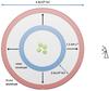 |
Fig. 9 Representation of the expanding envelope toward NGC 6334 I. See Sect. 5.3 for explanation. |
| In the text | |
|
Fig. 10 [HCO+]/[N2H+] abundance ratio as a function of the CR ionization rate computed for the inner (blue line) and outer (red line) envelope components using the Nahoon code. The shaded areas represent the results obtained within the uncertainties listed in Table 3. The ζH2 values in the upper-left and lower-right corners of the shaded areas correspond to the maximum and minimum values of the [HCO+]/[N2H+] ratio, respectively (see text for discussion). |
| In the text | |
Current usage metrics show cumulative count of Article Views (full-text article views including HTML views, PDF and ePub downloads, according to the available data) and Abstracts Views on Vision4Press platform.
Data correspond to usage on the plateform after 2015. The current usage metrics is available 48-96 hours after online publication and is updated daily on week days.
Initial download of the metrics may take a while.