| Issue |
A&A
Volume 563, March 2014
|
|
|---|---|---|
| Article Number | A119 | |
| Number of page(s) | 16 | |
| Section | Extragalactic astronomy | |
| DOI | https://doi.org/10.1051/0004-6361/201321989 | |
| Published online | 19 March 2014 | |
The HST view of the broad line region in low luminosity AGN⋆
INAF − Osservatorio Astrofisico di Torino, via Osservatorio 20, 10025 Pino Torinese, Italy
e-mail: This email address is being protected from spambots. You need JavaScript enabled to view it.
Received: 29 May 2013
Accepted: 8 January 2014
Abstract
We analyze the properties of the broad line region (BLR) in low luminosity AGN by using HST/STIS spectra. We consider a sample of 24 nearby galaxies in which the presence of a BLR has been reported from their Palomar ground-based spectra. Following a widely used strategy, we used the [S II] doublet to subtract the contribution of the narrow emission lines to the Hα+[N II] complex and to isolate the BLR emission. Significant residuals that suggest a BLR, are present. However, the results change substantially when the [O I] doublet is used. Furthermore, the spectra are also reproduced well by just including a wing in the narrow Hα and [N II] lines, thus not requiring the presence of a BLR. We conclude that the complex structure of the narrow line region (NLR) is not captured with this approach and that it does not lead to general robust constraints on the properties of the BLR in these low-luminosity AGN. Nonetheless, the existence of a BLR is firmly established in 10 objects, 5 Seyferts, and 5 LINERs. However, the measured BLR fluxes and widths in the 5 LINERs differ substantially with respect to the ground-based data. The BLR sizes in LINERs, which are estimated by using the virial formula from the line widths and the black hole mass, are clustered between ~500 and 2000 Schwarzschild radii (i.e., ~5−100 light days). These values are ~1 order of magnitude greater than the extrapolation to low luminosities of the relation between the BLR radius and AGN luminosity observed in more powerful active nuclei. We found BLR in objects with Eddington ratios as low as Lbol/LEdd ~ 10-5, with the faintest BLR having a luminosity of ~1038erg s-1. This contrasts with theoretical models that predict the BLR disappearance at low luminosity. We ascribe the larger BLR radius to the lower accretion rate in LINERs when compared to the Seyfert, which causes the formation of an inner region dominated by an advection-dominated accretion flow (ADAF). The estimated BLR sizes in LINERs are comparable to the radius where the transition between the ADAF and the standard thin disk occurs due to disk evaporation. We suggest that BLR clouds cannot coexist with the hot inner region and that they only form in the correspondence with a thin accretion disk.
Key words: galaxies: active / galaxies: Seyfert / galaxies: nuclei
Appendix A is available in electronic form at http://www.aanda.org
© ESO, 2014
1. Introduction
The clearest signature of an active galactic nucleus (AGN) is the presence of broad emission lines in its spectrum, produced by dense clouds of ionized gas located in the broad line region (BLR). The substantial line widths and rapid variability indicate that the BLR is located very close to the central source. Therefore, the BLR represents a unique laboratory for exploring the process of accretion onto supermassive black holes (SMBH). The BLR has been intensively studied for many years, but it is far from being completely understood. Several questions concerning, for instance, the origin of the BLR clouds, their dynamics, and the way they are related to the overall properties of the AGN are still waiting for an answer.
Log of the HST/STIS observations.
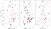 |
Fig. 1 Spectroscopic diagnostic diagrams for the galaxies of the Palomar sample with reported broad lines. The red (black) dots represent galaxies with (without) available HST spectra. The solid lines are from Kewley et al. (2006) and separate star-forming galaxies, LINER, and Seyfert; in the left panel, the region between the two curves is populated by the composite galaxies. |
The BLR is spatially unresolved in even the nearest AGNs, and the only information about its structure can be inferred from the properties of the broad emission lines. The most powerful method of exploring the geometry and kinematics of the BLR is the reverberation mapping technique, based on the time lag between the changes in the broad emission lines in response to the variation in the ionizing radiation (Blandford & McKee 1982). Among other results, reverberation mapping constrains the BLR size and offers the possibility of estimating the mass of the SMBH (e.g., Peterson & Wandel 2000). The relation linking the BLR radius and the AGN luminosity (e.g., Kaspi et al. 2005; Bentz et al. 2013) can then be used to estimate black hole masses from single-epoch measurements of luminosities and line profiles in all broad lined AGN, even at high redshift (Vestergaard 2002). Clearly, any improvement in the physical picture of the BLR would increase confidence in this extremely powerful tool.
The purpose of our study is to gain a deeper understanding of the BLR and of its link to the central engine by exploring its properties in low-luminosity AGNs (LLAGNs). While most of the observational and theoretical effort has been devoted to studying the BLR in luminous AGNs, LLAGNs can offer a different perspective. It is indeed becoming increasingly clear that LLAGNs are not simply scaled down versions of more powerful active galaxies, because at the lowest accretion levels, the mechanism of black hole feeding is likely to be substantially different. Given the strong connection between the accretion disk and the BLR predicted by most models, we might expect that the broad lines in LLAGNs should also be affected. For example, it has been proposed that the BLR disappears in these objects (e.g., Laor 2003; Nicastro 2000; Elitzur & Shlosman 2006), and it is then essential to establish whether this is indeed the case and at which level of activity this occurs.
A significant improvement in our knowledge of the BLR properties in LLAGNs has been achieved with the ground-based spectroscopic study of a complete sample of 486 nearby galaxies by Ho et al. (1997a,b), hereafter, the Palomar survey. These data are a fundamental reservoir of measurements for statistical studies of the nuclear properties of LLAGNs. However, the detection and the measurement of broad lines in the spectra of LLAGN is particularly difficult. Nonetheless, in their survey, the presence of a BLR has been reported in 46 objects, at various levels of confidence, of the 211 galaxies classified as Seyferts or LINERs (Ho et al. 1997c). Based mainly on these results, Wang & Zhang (2003) and Zhang et al. (2007) argue that the BLR size in LLAGNs is apparently larger than what it would have been expected given their luminosity. They suggest that this is due to a lower ionization (and/or a lower density) of the BLR clouds in these “dwarf” AGNs with respect to Seyfert 1 galaxies and QSOs.
However, the BLR properties of LLAGN obtained from observations with the STIS spectrograph on board HST differ, often dramatically, from what is seen in ground-based spectra (see, e.g., Ho et al. 2000; Shields et al. 2000; Barth et al. 2001; de Francesco et al. 2006). This might have been expected since ground-based spectra are affected by a strong stellar continuum level and by narrow lines contamination. HST/STIS is better suited to studying faint broad emission lines, thanks to the strongly reduced aperture size that enhances the contrast between weak, broad emission lines against the bulge starlight and the narrow lines. We here analyze the available HST/STIS spectra of the galaxies for which the presence of a broad Hα emission has been reported in the Palomar survey.
The paper is organized as follows. In Sect. 2 we define the sample of LLAGNs studied, while in Sect. 3 we present the analysis of the HST spectra and the main observational results. The properties of the detected BLR and the comparison with the ground-based results are presented in Sects. 4 and 5. We explore the detectability of the BLR in the objects where it is not seen in Sect. 6. In Sect. 7 we discuss whether the BLR scaling relations derived for luminous AGN can also be applied to LLAGNs. In Sect. 8 the properties of the BLR in LLAGN are compared to various models that predict its disappearance at low luminosities. In Sect. 9 we provide a summary and our conclusions.
Parameters of the sample galaxies.
2. The sample and the archival observations
The Palomar survey consists of optical spectroscopic observations, performed with the Palomar 5 m Hale telescope, of 486 bright (BT ≤ 12.5 mag) galaxies, located in the northern sky (Filippenko & Sargent 1985; Ho et al. 1995). In these ground-based spectra, 46 galaxies show definite or probable evidence of broad Hα emission (Ho et al. 1997c). We searched the Hubble Legacy Archive (HLA) for HST/STIS spectra of these sources covering the Hα line1 or, when not available, the Hβ region. We found data for 24 galaxies, as reported in Table 1.
When available, we combined multiple observations to remove cosmic rays and bad pixels. From the fully calibrated data we extracted the nuclear spectrum from a synthetic aperture of 0.̋15 and applied the proper aperture corrections.
The HST aperture is thus 0.̋2 (or even 0.̋1) × 0.̋15, which is significantly smaller than the 2″× 4″ aperture of the Palomar survey. This reduces the contamination of starlight and of narrow lines, favoring the detection of any broad line component. The dramatic change in our view of LLAGN when using HST spectra is described well by the comparison with the corresponding ground based spectrum (see Fig. 2).
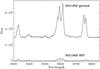 |
Fig. 2 Comparison of HST and Palomar spectra of NGC 1052. The fluxes are in unit of 10-18erg s-1 cm-2 Å-1, while wavelengths are in Å. |
We explored the location of these sources in the spectroscopic diagnostic diagrams (see Fig. 1) by using the ground-based emission line ratios. According to the criteria given by Kewley et al. (2006), 16 of them are LINERs, 7 Seyfert, and one (namely NGC 1275) is an ambiguous source, since it moves from the Seyfert region in the middle panel to the LINERs region, in the righthand panel (see Table 2).
3. Analysis of the spectra
In this section we describe the analysis of the spectra used to assess the presence of any broad component in the Balmer lines. In ten cases, a BLR is readily visible with just a visual inspection of the spectra. This is the case for all Seyfert galaxies (with the exception of NGC 3982 and NGC 4258, which is probably not a true Seyfert, as we discuss in Sect. 8) and of five LINERs. Their spectra are shown in Fig. 3 and are analyzed in more detail toward the end of this section.
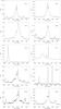 |
Fig. 3 Spectra of the objects in which a broad Balmer line is readily visible with just a visual inspection. |
The spectra of the remaining sources require a more accurate analysis before we can conclude whether a BLR is present and, in this case, derive its properties. The method we adopted is based on the assumption that the lines of the [S II] doublet provide a good representation of the shape of the [N II] and of the Hα narrow line component, similar to the method used by Ho et al. (1997c). The [S II] lines are reproduced with a Gaussian profile but, when needed, two Gaussians for each line are used.
For each source, we initially attempted to reproduce the Hα+[N II] complex by fixing the line’s shape to the one derived for the [S II] without including any broad Hα component by just scaling the line intensities to match the Hα and [N II]λ6584 line peaks (we recall that the ratio between the two [N II] lines is fixed). The result of this procedure is shown in the top lefthand panel of Fig. 4, by using NGC 1052 again as an example. Significant residuals are present in the form of blue and red wings around the Hα+[N II] complex, apparently a clear indication of the presence of a broad Hα component. We then include such a component in our analysis (Fig. 4, top right panel) by adopting a skewed Gaussian shape in this case. The free parameters (the intensities of all lines and the width of the broad component) are derived by minimizing the residuals. For the BLR in NGC 1052, we obtain a full width at half maximum (FHWM) of 2240 km s-1, a flux of 8.7 × 10⁻¹⁴ erg s-1 cm-2, and a skewness parameter of 0.06.
Rather different results are instead obtained when we use the [O I] doublet as template for the shape of the [N II] and Hα lines (Fig. 4, bottom left panel). The [O I] lines are in fact significantly broader than the [S II] ones (the FWHM are 660 km s-1 for [O I]and 570 for [S II], see Table 3). They also show much more developed wings on both the blue and red sides. As a result, the red end of the Hα+[N II] complex is perfectly reproduced by the shape of the [O I], while a broad component is still needed to account for its blue side. By comparing with the results obtained from the [S II] template, we note that while the FWHM of BLR is similar (~2200 km s-1), the BLR flux is reduced by a factor of 5 (see Table 4) and it is blue-shifted by ~1200 km s-1.
As a final test, we performed a fit in which a Gaussian blue wing is added to [O I] shape for each narrow component of the complex (see Fig. 4, bottom right panel), keeping the [N II]/Hα ratio fixed to the same value measured for the main component. This model reproduces the spectrum equally well as the fit that includes a BLR. The contribution of the blue wing increases only marginally the FW20 of the [N II] line, from 1320 km s-1 to 1370 km s-1.
Summarizing, in NGC 1052, including a broad Hα line improves the spectral fit obtained by using the [S II] (or the [O I]) lines as templates for the shape of [N II] and Hα; however, the results differ depending on which line is actually used, owing to the mismatch between the profiles of [S II] and [O I]. An equally satisfactory fit is achieved by adding a blue wing to the emission lines of the narrow Hα+[N II] complex.
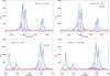 |
Fig. 4 Top left: spectrum of NGC 1052 modeled by adopting the same shape as obtained from the Gaussian fitting of the [S II] doublet for the Hα and [N II] lines. The Hα and [N II] intensities are set by matching their respective emission peaks. The original spectrum is in black, the individual lines are in blue, the total line emission in green, the residuals in red. Top right: same as in the left panel but including a broad Hα component (red). Bottom left: same as in the top right panel, but using the [O I] doublet as template. Bottom right: same as in the bottom left panel, but including blue wings to the narrow lines instead of a BLR. Wavelengths are in Å, while fluxes are in units of 10-18erg s-1 cm-2 Å-1. |
How general is this behavior? Such an analysis can be performed only when both the [S II] and [O I] doublets are covered by the HST spectrum and when their signal-to-noise ratio is sufficient for a reliable fit of their profiles. This is possible for the nine sources listed in Table 3. The main results obtained for NGC 1052 are confirmed:
-
i) the three fitting methods reproduce the data with similaraccuracy;
-
ii) the [O I] lines are generally broader than the [S II] lines (see Table 3, where the width at half maximum and at 20% intensity are compared);
-
iii) the [N II] and Hα wings required to reproduce the spectra increase the FW20 of these lines by less than 30%, and usually by less than 15%2;
-
iv) excluding the objects presented in Fig. 3 showing a clear BLR, the BLR flux obtained from cloning the [S II] are larger than when using the [O I] (see Table 4 where we compare the flux and width obtained in the two cases), while the widths are similar.
Forbidden line widths.
Broad line parameters from different templates.
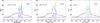 |
Fig. 5 Spectrum of a LINER with a clear BLR (NGC 4203) reproduced with a skewed Gaussian (red curve). The residual [N II]+Hα complex is modeled with 3 different methods: by cloning the [S II] doublet (left), by including a second broad Hα component (middle), or by using the [O I] doublet (right). The original spectrum is in black, the individual lines are in blue, the total line emission in green, the residuals in red. Wavelengths are in Å, while fluxes are in units of 10-18erg s-1 cm-2 Å-1. |
For the five LINERs with a clear BLR, the situation is similar, once this broad component is taken into account. We treat NGC 4203 in detail as an example. In this source there is a well defined broad Hα component, extending over ~15 000 km s-1. We reproduce this component with a skewed Gaussian (the resulting parameters are given in Table 2), obtained after masking the spectral region covered by the narrow [N II]+Hα complex.
We then attempt to reproduce the remaining emission in three different ways: i) using the [S II] as template without any further broad component (Fig. 5, right panel); ii) by adding a second broad Hα component (middle panel); and iii) by using the [O I] line as template (left panel). While a second broad component is clearly needed from the [S II] template, the fit obtained with the [O I] is already satisfactory. This is due to the fact that the [O I] lines are broader than the [S II], similar to the cases presented above. In the Fig. 6 we show the analysis for the four other LINERs with clear BLR. It leads to analogous results; i.e., no broad Hα line (in addition to its main component) is required to reproduce the data.
In seven galaxies the [O I] line is either not covered by the HST spectrum or is too faint to be modeled accurately. In these cases we can only rely on the [S II] lines as template. In Table 4 we report FWHM and fluxes of the broad Hα component. The relative fit are shown in Fig. A.2. The results obtained share several aspects with those presented before. In particular an accurate fit is also obtained by just adding a broad wing in both [N II] and Hα to the [S II] template. Furthermore, the widths of the broad lines are again clustered around a FWHM of ~2000 km s-1, being included between ~1000 and ~3000 km s-1. For NGC 4636 the data quality is insufficient to proceed to any reliable analysis. Its spectrum is shown in Fig. 7.
In three cases (namely NGC 4151, NGC 4395, and NGC 1275), there are no medium-resolution HST spectra covering the Hα region, and we then used spectra including the Hβ line. The separation between the emission lines in this spectral region is large enough that data from the low-resolution grism G430L can also be used. We adopted the same method described above, but by using the [O III]λ5007 as template for the shape of the Hβ line. This is an even less accurate assumption than the similarity of the [S II] and [N II] profiles, since [O III] is a high ionization line that might be produced in regions that are significantly different from the Balmer lines. However, this is not a significant issue since in two galaxies (namely NGC 4151 and NGC 4395), the presence of the broad Hβ is clearly visible and its properties are not significantly affected by the de-blending procedure. In the third case (i.e., the ambiguous galaxy NGC 1275), we failed to detect a broad Hβ component.
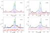 |
Fig. 6 Spectra of the LINERs with a clear BLR, in addition to NGC 4203 presented above, modeled using [O I] as template for the narrow lines. The broad Hα (red curve) is reproduced with a skewed Gaussian. The original spectrum is in black, the individual narrow lines are in blue, the total line emission in green, the residuals in red. Wavelengths are in Å, while fluxes are in units of 10-18erg s-1 cm-2 Å-1. |
4. The properties of the BLR in LLAGN
The results presented in the previous section indicate that there is a substantial mismatch between the profiles of the different emission lines considered. This is very likely due to a stratification in density and ionization within the narrow line region (NLR) that causes differences in the location of the emitting region for the various lines and, consequently, differences in the lines profiles. For example, the various lines considered are associated with different critical densities, with the [S II] lines having the lowest value3. Several indications for the presence of a dense, compact emitting region within the NLR, located within a radius of a few pc from the central black hole are emerging (Capetti et al. 2005; Peterson et al. 2013; Baldi et al. 2013). It can be envisaged that this region is poorly represented in the [S II] profile, while it is more prominent for the [O I], owing to its higher critical density. On the other hand, the possible presence of blue wings in the [N II] profile, with respect to [O I], might be due to an ionization stratification of the NLR.
The complex structure of the NLR is not completely captured with the approach usually followed to model the [N II]+Hα complex by using different forbidden emission lines as templates. In this situation, the properties of the BLR obtained with this procedure, including its very detection, must be treated with caution. In particular, the need for a BLR based only on the improvement in the fit when such a component is added is highly questionable: it might not imply that a broad component is really present, but it could be just the consequence of the complex NLR structure not fully represented by the templates. The similarity in the quality of the fit with the three methods presented (by using the [S II] or [O I] as templates, or adding a broad base wing to them) casts doubts on the reliability of the BLR detections.
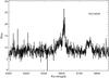 |
Fig. 7 Spectrum of NGC 4636. The signal-to-noise ratio is insufficient for any reliable analysis of this source. |
The other indication against the reality of the broad Hα is the strong clustering of the derived values for their widths. The values derived for the LINERs considered are typically of ~2000 km s-1. This is intriguingly similar to the value that corresponds to the separation of the two lines of the [N II] doublet, 1650 km s-1. Indeed, any positive residual left after the subtraction of a template will be distributed over a spectral region corresponding to the observed values. We then adopt the fluxes of the BLR obtained with the [S II] (or [O I]) template as conservative upper limits, rather than genuine detections.
The values reported in Table 2 are strictly valid only for the FWHM quoted in Table 4, i.e., ~2000 km s-1. We then also explored the dependence of this limit on the BLR width, by repeating the fit procedure with the FWHM fixed at various values, ranging from 3000 to 30 000 km s-1. We find that the limit on the BLR flux has a complex relation with its width, but with some common feature from source to source. Despite the increasing width, the limit initially decreases because when the broad line wings exceed the width of the [N II]+Hα complex, the BLR would become readily visible even for relatively low intensities. For higher values, FWHM ~ 4000 − 15 000, it increases almost linearly. However, for FWHM ≳ 15 000 km s-1, the spectral gradient becomes too small to separate any BLR from the continuum and the BLR flux sharply increases. We return to this issue in Sect. 6.
For the LINERs in which the BLR is instead visible, there is a similar effect. There is not a disappearance of the whole BLR, but only of its relatively narrow core (again with FWHM ~ 2000 km s-1) superposed on a broad Hα base.
The HST spectra of these objects have already been presented and analyzed (NGC 3031, Devereux et al. 2003; NGC 3998, de Francesco et al. 2006; NGC 4203, Shields et al. 2000; NGC 4450, Ho et al. 2000; NGC 4579, Barth et al. 2001; but see also Walsh et al. 2008; Rice et al. 2006; Shields et al. 2007). These authors used slightly different fitting strategies to deblend the broad line emission: for example Ho et al. (2000) and Shields et al. (2000) reproduce the narrow the [N II]+Hα complex with a synthetic [S II] profile. They interpret the residual of the fit as a combination of a “normal” broad line (with a width of ~2000 km s-1, similar to those observed from the ground) superposed on a double-peaked emission with high velocity wings. As explained above, we argue that the “normal” BLR is actually due to the mismatch between the lines in the [N II]+Hα complex and the templates used. While this affects the BLR profiles, the BLR fluxes they obtained are similar to ours.
In Table 2 we report fluxes (or upper limits) and widths (in case of detections) obtained for the broad Balmer lines.
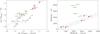 |
Fig. 8 Logarithmic fluxes (left, in erg s-1 cm-2) and full width at half maximum (right, in km s-1) of the Hα broad line emission obtained from the HST/STIS spectra compared to the results of the Palomar spectroscopic survey. The dashed line has a slope equal to one. The green symbols represent the LINERs of the sample, while the red squares are the Seyferts. NGC 1275, the ambiguous galaxy, is marked with a purple square. Empty symbols refer to the undetected BLR. |
5. Comparison with ground-based measurements
In Fig. 8 we compare the BLR fluxes measured from HST and ground-based spectra. We confirm the presence in the HST spectra of a broad Balmer line emission in all Seyferts but one. Their HST line fluxes, ranging from ~10-13 to ~10-11 erg s-1 cm-2, are all very similar to the ground-based measurements, typically differing by less than a factor of 1.5. The only exception is NGC 3982, the Seyfert galaxy with the largest absorbing column density in X-rays (NH ~ 4.3 × 1023 cm-2, Akylas & Georgantopoulos 2009) of the sample. Most likely, the lack of a BLR is due to nuclear obscuration. From the point of view of broad lines widths, in the right panel of Fig. 8 we compare the FWHM of the broad Hα emission line obtained from the HST and ground-based spectra. For the Seyferts, the differences are all less than 500 km s-1, with the only exception of NGC 4151. However, for this object, we show the width of the Hβ line, properly corrected4. Nonetheless, inspection of the Palomar spectrum shows that in this object the Hβ is indeed significantly broader than the Hα and in good agreement with the HST measurement.
The situation for the LINERs is quite different. We initially concentrate on the five objects with a clear BLR. First of all their BLR are generally of lower fluxes than in Seyferts, from ~10-13 to ~10-12 erg s-1 cm-2. The spread of the ratios between HST and ground measurements for the detected sources is much larger, ranging from 0.3 to 20. All HST measurements of the FWHM are in strongly excess with respect to the ground-based data. While the ground-based data indicate widths between 1500 and 3000 km s-1, much broader lines are seen in the HST data with FWHM reaching 8000 km s-1. As explained above, we argue that the ground-based BLR detections are spurious. The genuine broad emission lines in these sources (as previously noted by Ho et al. 2000 for NGC 4203; Shields et al. 2000 for NGC 4450; and de Francesco et al. 2006 for NGC 3998) are not visible in ground-based spectra, owing to the higher continuum and narrow line fluxes.
In the galaxies without a clear BLR, the ground-based measurements are usually higher than the flux obtained from the HST data, by a factor of up to 10. Particularly instructive is the comparison between the broad Hα line derived from the ground- based data of NGC 1052, shown in Fig. 9, that indicates that the ground-based BLR is inconsistent with the data, regardless of the modeling scheme, since it exceeds the whole flux of the [N II]+Hα complex.
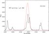 |
Fig. 9 Broad Hα line derived from the ground based data of NGC 1052 (red Gaussian) compared to the HST spectrum. |
6. On the detectability of BLR in LLAGN
In most of the LINERs we considered, the presence of a BLR is not readily visible and it is not required by the analysis of their spectra. Is the BLR really missing, or they are just too faint to be detected?
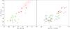 |
Fig. 10 BLR luminosity against 2 AGN power estimators: the [O III] narrow line luminosity (left panel) and the intrinsic X-ray luminosity corrected for absorption in the 2−10 keV band (right panel). The green circles represent LINERs, the red squares are the Seyferts (empty symbols refer to the undetected BLR), the red dots are the objects from Marziani et al. (2003). |
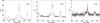 |
Fig. 11 Comparison of the HST spectrum with two predicted BLR synthetic profile for NGC 1052 (left), NGC 4278 (center), and NGC 4636 (right). The blue curve represents a BLR with flux derived from the X-ray flux and a width of 6500 km s-1, conservatively reduced by a factor 10 to explore its detectability in the HST spectrum. The normalization of the red curve is derived from the [O III] flux, in this case reduced by a factor of 3. |
To answer to this question in Fig. 10 we compare the broad Hα luminosity with two estimators of the AGN power, i.e., the luminosity of the [O III] narrow line and the unabsorbed nuclear X-ray luminosity in the 2−10 keV band, see Table 2. A strong trend is clearly present in all comparisons. This might have been expected since both the NLR and the BLR are photoionized by the AGN continuum, that is estimated well by its X-ray. The LINERs smoothly extend the relation seen in more powerful AGN, representing the low-luminosity end of the distributions in all diagrams. The median ratio between the BLR and the X-ray luminosities measured in the ten objects with a clear BLR is LBLR/LX ~ 0.08 (and LBLR/L[O III] ~ 3). All ten data points fall within a factor of 10 of the median value (and within a factor of three considering the relation linking LBLR and L[O III]). We then predict the BLR luminosity in the objects apparently without broad lines by assuming that it follows these multiwavelength trends.
The BLR widths can be instead derived from the virial formula, by adopting the scaling relations of more powerful AGN and the BLR luminosity just derived. We find that such BLR could not be detected in any source, because of the extremely high line widths whose median is of ~30 000 km s-1.
We also consider another possibility, i.e., that the BLR radius has the same value, RBLR ~ 1000rs, shown by the 5 LINERs with a clear BLR. This simply corresponds to widths similar to those observed and we adopt the average value of 6500 km s-1. In this case the BLR should be readily visible in 5 of the 12 LINERs considered. In order to account for the observed scatter in the ratios used to estimate the BLR luminosity, we reduced conservatively all the predicted BLR fluxes by a factor of 10 for those derived from the LBLR/LX ratio and by a factor of 3 for those estimated from the LBLR/L[O III] ratio. The BLR should be still detected in three objects, namely NGC 1052, NGC 4278, and NGC 4636, according to both estimates, see Fig. 11.
7. The BLR scaling relations in LLAGN
Reverberation studies of AGN revealed that the BLR properties are strongly linked to those of the AGN and of the central black hole. Time lag measurements between changes in the continuum and broad lines lead to estimates of the BLR radius, RBLR. The SMBH mass can thus be derived from the virial formula, relating the SMBH mass with the BLR width and its radius in the form MBH = f G-1 FWHM2RBLR. The factor f is empirically determined to match the SMBH masses derived with the reverberation technique and the values obtained from the measurements of stellar velocity dispersions σ⋆ (Ferrarese & Merritt 2000; Gebhardt et al. 2000)5. Furthermore, reverberation mapping measurements show a close connection between the BLR radius and the AGN continuum luminosity (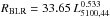 lt-days, where L5100,44 is the luminosity at 5100 Å in units of 1044erg s-1, Bentz et al. 2013).
For LLAGN the situation is somewhat different. In fact, the reduced contribution of the active nucleus, with respect to more powerful AGN, enables us to estimate their black hole mass from measurements of the stellar velocity dispersion σ⋆. Furthermore, the measurements of the optical continuum are severely contaminated by the starlight, particularly in the least luminous AGN. This is clearly shown by the strong stellar absorption features visible in their blue HST spectra (see, e.g., Sarzi et al. 2005). Therefore, their optical continuum luminosity cannot be used to test the validity of the scaling relations obtained for more powerful AGNs in LLAGN.
Nonetheless, having estimated the SMBH mass6, we can invert the virial formula and use it to estimate the BLR radius:
 In Fig. 12 we compare the BLR radius with its luminosity7 for the ten LLAGNs with a detected BLR. The BLR radius is typically ~10 lt-days, but it reaches for a value of 100 lt-days NGC 3998.
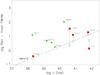 |
Fig. 12 BLR radius (in light-days) against Hα luminosity (in erg s-1 units). The dashed lines represent BLR radius–luminosity relations derived from the law linking RBLR with the continuum luminosity (Bentz et al. 2013). The green circles are LINERs, the red squares Seyferts. The arrows point to the reverberation mapping measurement of RBLR, when available (Bentz et al. 2013). |
For a comparison with the more powerful AGN, we can rely on the strong relation between L5100 and Hα emission line luminosity (Greene & Ho 2005); i.e.,  (in 1042 erg s-1 units), which in this case includes both the broad and narrow Hα emission. By combining this relation with that derived by Bentz et al. we can derive the law linking the BLR radius to the Hα luminosity; i.e.,
  lt-days. This relation is reported in Fig. 12 as a dashed-dotted line.
The 5 Seyferts in the Palomar sample generally follow, with some scatter, the relation BLR radius–luminosity relation of the sample of Seyfert and quasars with reverberation mapping measurements (that actually includes all but 1 of the Seyfert considered here). For the LINERs galaxies we instead obtained BLR radii always larger than predicted by the LHα − RBLR relation. The median excess is of ~1 order of magnitude. We conclude that LINERs do not follow the BLR scaling relations defined by the more luminous AGN. In the following Section we investigate the origin of this result.
8. Comparison with BLR theoretical models
Several models predict that for accretion rate or bolometric luminosity below a threshold limit, the BLR and the standard torus cease to exist. We consider the predictions of three such models in detail and compare them with our results. According to Nicastro (2000) the BLR forms from disk instabilities in correspondence of the transition radius from density- to radiation-dominated regions. For bolometric luminosities lower than Lbol < 0.024 (MBH/M⊙)− 1/8 LEdd, this radius is smaller than the last stable orbit and the BLR cannot be present.
According to Laor (2003), the BLR clouds are disrupted when the velocity of BLR clouds exceeds Δv > 25 000 km s-1. For the BLR radius–luminosity relation, at low luminosity the RBLR shrinks and Δv exceeds this threshold, and the BLR cannot form. This occurs at a luminosity of Lbol < 1041.8(MBH/108M⊙)2erg s-1.
In the scenario of Elitzur & Shlosman (2006), the torus and the BLR are smoothly connected, with the BLR formed by an outflow of ionized gas from the accretion disk that extends outward until the dust sublimation radius, the inner boundary of the dusty, and clumpy torus. The column density required for the formation of the BLR and the torus are achieved only for high Eddington ratios and both the BLR and the torus disappear when the bolometric luminosity falls below Lbol < 1042erg s-1.
These models predict different dependencies on the bolometric luminosity and the black hole mass (or equivalently on Eddington luminosity), below which a BLR cannot form, but all agree that BLR cannot exist in object with bolometric luminosity lower than Lbol ≲ 1042 erg s-1 and black hole mass higher than MBH ≳ 107 − 108M⊙ (see Fig. 13). All these models fail to predict the presence of a BLR in the two least luminous LINERs with a clear BLR. This confirms on different grounds that the scaling relations between BLR and AGN (implicitly assumed by all the models) do not properly predict the properties of broad emission lines in LINERs.
In Sect. 6 we showed that the LINERs smoothly extend the relations that, in more powerful AGN, link the nuclear and the BLR power, representing the low end of the luminosity distributions. However, the LINERs of our sample are not simply scale-downed versions of Seyfert galaxies. In Fig. 14, we show the distributions of the Eddington ratios for the two types of AGN. We apply a bolometric correction to the nuclear X-ray luminosity of 16 (i.e., Lbol = 16 LX, Ho 2008). LINERs and Seyferts are well separated, in line with results obtained previously from the analysis of larger AGN samples (e.g., Kewley et al. 2006). The overlap between the two classes is only due to NGC 4258 and NGC 3982. As discussed above, the measurements for NGC 3982 are not reliable because of nuclear obscuration. The second object is NGC 4258 for which we argue that the identification as Seyfert is questionable. Indeed, the HST spectrum shows that the [S II]/Hα and [O I]/Hα ratios are higher that what is found in the Palomar data. In particular, we measure [O I]/Hα = 0.96, which locates NGC 4258 well into the LINERs region, regardless of its [O III]/Hβ ratio8.
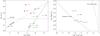 |
Fig. 13 Left panel: limits for the presence of a BLR from Elitzur & Shlosman (2006), Laor (2003), and Nicastro (2000). These models predict that objects located in the portion of the plane below the dashed lines cannot form a BLR. Left panel: predictions on the transition radius between the geometrically thick and thin regions of the accretion disk in a pure ADAF model and Evaporation model (models A and C from Czerny et al. 2004, adopting α = 0.1 and β = 0.99, see text). |
 |
Fig. 14 Distribution of the ratio between bolometric luminosity (estimated as ~16 LX) and Eddington luminosity for LINERs (green) and Seyferts (red). The empty regions of the histograms represent objects with undetected BLR. |
Various models predict that below a given threshold in Eddington ratio (Lbol/LEdd≲ 0.01), the radiatively efficient accretion disk (geometrically thin and optically thick), which is typical of powerful AGNs, changes its structure into an inner hot and radiatively inefficient flow (optically thin and geometrically thick), possibly an advection-dominated accretion flow, ADAF, (e.g., Narayan & Yi 1995) while only at large radii does the standard disk survive. Application of an ADAF model to the SED of low luminosity AGNs suggests a transition radius (between the inner ADAF and the outer disk) on the order of Rtr ~ 100 − 1000 rs, (Ho 2008)9, to explain the absence of the so-called “blue bum”, the excess in the UV continuum typical of Seyferts galaxies.
From a theoretical point of view, the hot corona is truncated at the radius where the ADAF solutions ceases to exist. Following Czerny et al. (2004), the truncation radius is given by
 (model A in Czerny et al. 2004, where α is the viscosity parameter, and
  is the accretion radiative efficiency, function of model parameters and of the accretion rate).
However, taking the process of evaporation of the cold disk in the ADAF into account, and assuming a two-temperature model of the corona (“Evaporation model C” in Czerny et al. 2004), one obtains a different prescription for the transition radius:
 where β is ratio of the gas pressure to the total (gas+magnetic) pressure.
In Fig. 13 we report the dependence of the transition radius on the Eddington ratio predicted by the two models and compare it with the estimated BLR radii for LINERs. We find the RBLR values in LINERs are clustered in the range 500−2000 rs. This is much lower than the truncation radii predicted by the pure ADAF model, but they are comparable to the values of the transition radii obtained from the evaporation model10.
This supports earlier suggestions (e.g., Czerny et al. 2004; Liu & Taam 2009) that the broad line clouds do not form (or cannot survive) within the hot part of the accretion flow, i.e., below the transition radius. Conversely, the BLR appears to naturally form in the presence of a thin (and relatively “cold”) accretion disk, which, in the case of LINERs, represents the outer portion of the disk structure.
This offers an explanation for the discrepancies found for LINERs behavior with respect to more powerful AGN and the violation of the BLR scaling relations. Indeed the BLR radii estimated for the LINERs from such relations would be ~ 0.3 and 3 lt-days (i.e., between ~30 and 250 rs for a 108 MBH, ⊙ black hole), well below the values obtained for the transition radii of the hot corona. We suggest that the BLR radius in these objects is not set by the AGN luminosity but from the presence of an inner forbidden region.
It is also interesting to estimate the dust sublimation radius. This is given by  pc, assuming a sublimation temperature of 1500 K (Barvainis 1987). For the LINERs considered here we obtain Rdust ~ 0.4 − 10 lt-days (and this must be considered as an upper limit, since our optical luminosities might be overestimated). These values are well within the ADAF region and much less than the BLR radii. This suggests that the structure of circum-nuclear tori in these sources (if at all present) differ profoundly from those seen in more powerful AGN. The likely absence of a standard Seyfert-like torus in low luminosity AGNs is also confirmed by high resolution MIR observations (Mason et al. 2012). The authors suggest that LLAGN may have a dust-to-gas ratio lower than most Seyfert galaxies, consistent with a disk wind scenario, in which at low Eddington ratio, the torus may be optically thin or may contain fewer clouds than a standard torus.
9. Summary and conclusions
We explored the properties of the BLR in low luminosity AGNs by using archival HST/STIS spectra. We considered the objects in which the presence of broad lines has been reported from their Palomar ground-based spectra. High spatial resolution data, such as those obtained with HST, are essential to achieving reliable measurement of the properties of the BLR, especially for low luminosity AGN. Indeed the smaller aperture of HST, which is more than ~100 times smaller than the aperture of the Palomar survey, allows us to decrease the stellar continuum and reduce the narrow line contamination.
In the HST archive we found data for 16 LINERs, 7 Seyferts, and 1 ambiguous galaxy. We separated the broad line from the Hα+[N II] narrow line complex by applying the shape of the de-blended lines profile of the [S II] doublet and by scaling the line intensity in order to match the Hα+[N II] peaks.
We confirm the presence of broad line emission in all but one Seyfert: the HST line widths are similar to those derived from the Palomar observations, while the fluxes typically differ by less than a factor 1.5 from the ground-based data. The only exception is NGC 3982, a source with a highly absorbed nucleus in the X-ray, where the BLR is most likely obscurated.
The discrepancies between HST and ground-based measurements are instead remarkable for LINERs. Only in five LINERs is a BLR is readily visible in the HST spectra. However, there is a large spread between the HST and ground-based data, with the fluxes differing by a factor ranging from 0.3 to 20; furthermore, the HST measurements of the line widths (between 4200 and 8000 km s-1) are substantially larger than the ground-based FWHM (with all widths in the range 1500−3000 km s-1).
Conversely, we do not find convincing evidence of a BLR in the remaining 14 sources. A BLR must generally be included to obtain a good fit to their spectra when using the [S II] lines as template for the [N II] and the narrow component of the Hα. However, if we instead use the [O I] lines we obtain rather different results, because the [O I] lines are broader than the [S II] lines. Furthermore, the spectra are also reproduced well without any BLR but by just adding a blue wing to the [N II] and narrow Hα lines.
This is likely due to a stratification in density and ionization within the NLR that causes differences in the location of the emitting region for the various lines and, consequently, differences in the lines profiles. For example, the existence of a compact and dense emitting region, located within a radius of a few pc from the central black hole, is supported by various studies. This region is poorly represented in the [S II] profile owing to the low critical density associated with this transition.
We conclude that complex structure of the NLR is not captured with the technique of spectral fitting based on the narrow line templates that it does not return, in general, robust constraints on the properties of the BLR in these low luminosity AGN.
For the ten galaxies in which instead a BLR is clearly detected, we estimated its radius by assuming the dominance of gravitational motions, i.e., by applying the virial formula, knowing the value of the σ-derived black hole mass and the broad line width. The resulting BLR radii in the five LINERs are clustered around ~1000 Schwarzschild radii (i.e., ~3 − 100 light-days). These values are significantly higher, by a factor of ~10 to 100, than the extrapolation to low luminosities of the scaling relations linking radio and luminosity of the BLR.
Our preferred interpretation to account for this inconsistency relies on the change in the accretion disk structure at low luminosities. LINERs differ from Seyfert for their lower accretion rates, causing the formation of an inner region dominated by an advection-dominated accretion flow (ADAF). The location of the transition radius between the ADAF region and the outer thin disk predicted by the evaporation model compares favorably with the estimated BLR radii for LINERs. This confirms earlier predictions that the BLR cannot coexist with the hot inner region and that they form (or survive) only in the presence of a thin accretion disk. As a result, LINERs do not obey the scaling relation defined by more powerful AGN.
The structure of circumnuclear tori, if at all present in these sources, must also differ profoundly from those seen in more powerful AGN since the estimated dust sublimation radii are smaller than the BLR size.
An interesting result of this study is that, despite the differences in BLR structure between LINERs and Seyfert, there is a continuity between the relations between BLR luminosity and AGN power for the two groups. This implies that the BLR covering factor is similar for the two classes of AGN. Nonetheless, a BLR is not readily visible in most LINERs. We used the relations linking the BLR and the AGN power to predict the broad line luminosity, hence whether the BLR in these objects should instead be seen. We find that the BLRs could not be detected if their widths follow the scaling relation of more powerful AGN, because of the extremely large FWHM, predicted to have a median value of ~30 000 km s-1. However, if the BLR radius in LINERs has a constant value, RBLR ~ 1000 rs, broad lines should be easily observed in at least three LINERs, based on their multiband luminosities. This might suggest that the BLR in LINERs are transient phenomena. We also note that the three objects where we would have expected to see a BLR are all radio-loud galaxies.
An important step forward for a better understanding of the BLR in LLAGNs can come from variability and reverberation mapping studies of these objects. They can provide us with a direct estimate of the BLR size, proofing or refuting our estimates based on the virial formula. Indeed, our assumption of the dominant role of the gravitational motions should be tested, and the role of various effects (e.g., related to the presence of winds or to the importance of radiation pressure) must be assessed. For example, it might be envisaged that the BLR in LINERs has a pure wind origin, lacking a rotating disk component, and consequently invalidating our analysis.
Online material
Appendix A: Spectral modeling
In this appendix we report the result of modeling the objects where the BLR is not clearly visible in their spectra. For four galaxies, the spectra cover the [O I] spectral region, and these lines are bright enough to allow us to use them as templates. In these cases, we modeled the spectra with three different methods 1) by using the [O I] lines as templates and including a broad
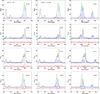 |
Fig. A.1 Modeling of the spectra of 4 objects without a readily visible BLR modeled with 3 different methods: by using the [O I] lines as templates and including a broad Hα component (left column), again with the [O I] template but adding a wing to the [N II] and narrow Hα lines (center column), by using as template the [S II] lines and including a BLR (right column). The original spectrum is in black, the contribution of the individual narrow lines in blue (their sum is in green), and in red are the residuals. The BLR component is in red. |
Hα component; 2) by using the [O I] template but adding a wing to the [N II] and narrow Hα lines and 3) by using the [S II] lines as template and including a BLR. For the eight remaining galaxies, the spectra do not cover the [O I] spectral region or these lines are not bright enough to be used as templates. In these cases we modeled the spectra with two different methods by using the [S II] lines as templates and 1) including a broad Hα component or 2) adding a wing to the [N II] and narrow Hα lines.
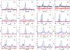 |
Fig. A.2 Analysis of the spectra 8 objects without a clear BLR and not covering the [O I] region (or with faint [O I] lines). Each spectrum is modeled with 2 methods, always using the [S II] lines as templates and (left) including a broad Hα component (right) or adding a wing to the [N II] and narrow Hα lines. The original spectrum is in black, the contribution of the individual narrow lines in blue (their sum is in green), and the residuals in red. In red we also show either the BLR component or the wings’ contribution. |
The spectral resolution of the G750L grism is insufficient for our purposes so we selected only data obtained with the medium-resolution grism G750M.
The only partial exception is NGC 4143. In this source the [O I] lines are broader than the [N II] and the required additional Gaussian component is a narrow core of the line, statistically preferred to a broad wing. In this case the red end of the [N II]+ Hα complex should be reproduced with a further component.
The logarithms of critical densities, in cm-3 units, are ~3.2, 3.6, 6.3, and 4.9 for [S II]λ6716, [S II]λ6731, [O I]λ6300, and [N II]λ6584, respectively (Appenzeller & Oestreicher 1988).
We convert the Hβ luminosity and width tabulated in this catalog to Hα luminosity using L(Hα) = 3.5 × L(Hβ) and FWHM(Hβ) = 1.07 ×FWHM(Hα)1.03, (Greene & Ho 2005).
Onken et al. (2004) estimated a correction factor f = 5.5 when using the second moment of the line profile in the virial formula. Since Peterson et al. (2004) found a mean ratio between FWHM and the second moment of 2.03, we then adopt f = 5.5/2.032 = 1.3.
We adopt the formulation of Tremaine et al. (2002),  , where σ⋆ ,200 is in 200 km s-1 units.
We use here the total Hα luminosity, including the broad and narrow components, although the latter contributes only less than ~10%.
This result is similar to what is found for NGC 5252, an object with a LINER nuclear spectrum, and a large scale line emission with ratios typical of Seyferts (Goncalves et al. 1998). The separation between the two classes occurs at Lbol/LEdd ~ 10-3.
Equivalent to Rtr ~ 1.14 (10-8−10-7)MBH in light-days.
We adopted a viscosity parameter α = 0.1 and a magnetic parameter β = 0.99. The “model C” curve shifts downward by only ~0.1 dex for, e.g., α = 0.04, and upward by ~0.9 dex for, e.g., β = 0.1; therefore, the transition radii are quite sensitive to the magnetic field strength.
Acknowledgments
We are grateful to the anonymous referee for usuful comments that significantly improved the paper. This work was mainly supported by the Italian Space Agency through contracts ASI-INAF I/009/10/0 and ASI/GLAST I/017/07/0.
References
- Akylas, A., & Georgantopoulos, I. 2009, A&A, 500, 999 [NASA ADS] [CrossRef] [EDP Sciences] [Google Scholar]
- Appenzeller, I., & Oestreicher, R. 1988, AJ, 95, 45 [NASA ADS] [CrossRef] [Google Scholar]
- Baldi, R. D., Capetti, A., Buttiglione, S., Chiaberge, M., & Celotti, A. 2013, A&A, 560, A81 [NASA ADS] [CrossRef] [EDP Sciences] [Google Scholar]
- Barth, A. J., Ho, L. C., Filippenko, A. V., Rix, H.-W., & Sargent, W. L. W. 2001, ApJ, 546, 205 [NASA ADS] [CrossRef] [Google Scholar]
- Barvainis, R. 1987, ApJ, 320, 537 [NASA ADS] [CrossRef] [Google Scholar]
- Bentz, M. C., Denney, K. D., Grier, C. J., et al. 2013, ApJ, 767, 149 [NASA ADS] [CrossRef] [Google Scholar]
- Blandford, R. D., & McKee, C. F. 1982, ApJ, 255, 419 [NASA ADS] [CrossRef] [EDP Sciences] [Google Scholar]
- Capetti, A., Verdoes Kleijn, G. A., & Chiaberge, M. 2005, A&A, 439, 935 [NASA ADS] [CrossRef] [EDP Sciences] [Google Scholar]
- Czerny, B., Rózańska, A., & Kuraszkiewicz, J. 2004, A&A, 428, 39 [NASA ADS] [CrossRef] [EDP Sciences] [Google Scholar]
- de Francesco, G., Capetti, A., & Marconi, A. 2006, A&A, 460, 439 [NASA ADS] [CrossRef] [EDP Sciences] [Google Scholar]
- Devereux, N., Ford, H., Tsvetanov, Z., & Jacoby, G. 2003, AJ, 125, 1226 [NASA ADS] [CrossRef] [Google Scholar]
- Elitzur, M., & Shlosman, I. 2006, ApJ, 648, L101 [NASA ADS] [CrossRef] [Google Scholar]
- Ferrarese, L., & Merritt, D. 2000, ApJ, 539, L9 [NASA ADS] [CrossRef] [Google Scholar]
- Filippenko, A. V., & Sargent, W. L. W. 1985, ApJS, 57, 503 [NASA ADS] [CrossRef] [Google Scholar]
- Gebhardt, K., Bender, R., Bower, G., et al. 2000, ApJ, 539, L13 [NASA ADS] [CrossRef] [Google Scholar]
- Gonçalves, A. C., Véron, P., & Véron-Cetty, M.-P. 1998, A&A, 333, 877 [NASA ADS] [Google Scholar]
- Greene, J. E., & Ho, L. C. 2005, ApJ, 630, 122 [NASA ADS] [CrossRef] [Google Scholar]
- Gültekin, K., Cackett, E. M., Miller, J. M., et al. 2012, ApJ, 749, 129 [NASA ADS] [CrossRef] [Google Scholar]
- Ho, L. C. 2008, ARA&A, 46, 475 [NASA ADS] [CrossRef] [Google Scholar]
- Ho, L. C. 2009, ApJ, 699, 626 [NASA ADS] [CrossRef] [Google Scholar]
- Ho, L. C., Filippenko, A. V., & Sargent, W. L. 1995, ApJS, 98, 477 [NASA ADS] [CrossRef] [Google Scholar]
- Ho, L. C., Filippenko, A. V., & Sargent, W. L. W. 1997a, ApJS, 112, 315 [NASA ADS] [CrossRef] [Google Scholar]
- Ho, L. C., Filippenko, A. V., & Sargent, W. L. W. 1997b, ApJ, 487, 568 [NASA ADS] [CrossRef] [Google Scholar]
- Ho, L. C., Filippenko, A. V., Sargent, W. L. W., & Peng, C. Y. 1997c, ApJS, 112, 391 [NASA ADS] [CrossRef] [Google Scholar]
- Ho, L. C., Rudnick, G., Rix, H.-W., et al. 2000, ApJ, 541, 120 [NASA ADS] [CrossRef] [Google Scholar]
- Ho, L. C., Greene, J. E., Filippenko, A. V., & Sargent, W. L. W. 2009, ApJS, 183, 1 [NASA ADS] [CrossRef] [Google Scholar]
- Kaspi, S., Maoz, D., Netzer, H., et al. 2005, ApJ, 629, 61 [NASA ADS] [CrossRef] [Google Scholar]
- Kewley, L. J., Groves, B., Kauffmann, G., & Heckman, T. 2006, MNRAS, 372, 961 [NASA ADS] [CrossRef] [Google Scholar]
- Laor, A. 2003, ApJ, 590, 86 [NASA ADS] [CrossRef] [Google Scholar]
- Liu, B. F., & Taam, R. E. 2009, ApJ, 707, 233 [NASA ADS] [CrossRef] [Google Scholar]
- Marziani, P., Sulentic, J. W., Zamanov, R., et al. 2003, ApJS, 145, 199 [NASA ADS] [CrossRef] [Google Scholar]
- Mason, R. E., Lopez-Rodriguez, E., Packham, C., et al. 2012, AJ, 144, 11 [NASA ADS] [CrossRef] [Google Scholar]
- Narayan, R., & Yi, I. 1995, ApJ, 444, 231 [NASA ADS] [CrossRef] [Google Scholar]
- Nicastro, F. 2000, ApJ, 530, L65 [NASA ADS] [CrossRef] [PubMed] [Google Scholar]
- Onken, C. A., Ferrarese, L., Merritt, D., et al. 2004, ApJ, 615, 645 [NASA ADS] [CrossRef] [Google Scholar]
- Peterson, B. M., & Wandel, A. 2000, ApJ, 540, L13 [NASA ADS] [CrossRef] [Google Scholar]
- Peterson, B. M., Ferrarese, L., Gilbert, K. M., et al. 2004, ApJ, 613, 682 [NASA ADS] [CrossRef] [Google Scholar]
- Peterson, B. M., Denney, K. D., De Rosa, G., et al. 2013, ApJ, 779, 109 [NASA ADS] [CrossRef] [Google Scholar]
- Rice, M. S., Martini, P., Greene, J. E., et al. 2006, ApJ, 636, 654 [NASA ADS] [CrossRef] [Google Scholar]
- Sarzi, M., Rix, H.-W., Shields, J. C., et al. 2005, ApJ, 628, 169 [NASA ADS] [CrossRef] [Google Scholar]
- Shields, J. C., Rix, H.-W., McIntosh, D. H., et al. 2000, ApJ, 534, L27 [NASA ADS] [CrossRef] [Google Scholar]
- Shields, J. C., Rix, H.-W., Sarzi, M., et al. 2007, ApJ, 654, 125 [NASA ADS] [CrossRef] [Google Scholar]
- Tremaine, S., Gebhardt, K., Bender, R., et al. 2002, ApJ, 574, 740 [NASA ADS] [CrossRef] [Google Scholar]
- Vestergaard, M. 2002, ApJ, 571, 733 [NASA ADS] [CrossRef] [Google Scholar]
- Walsh, J. L., Barth, A. J., Ho, L. C., et al. 2008, AJ, 136, 1677 [NASA ADS] [CrossRef] [Google Scholar]
- Wang, T.-G., & Zhang, X.-G. 2003, MNRAS, 340, 793 [NASA ADS] [CrossRef] [Google Scholar]
- Zhang, X.-G., Dultzin-Hacyan, D., & Wang, T.-G. 2007, MNRAS, 374, 691 [NASA ADS] [CrossRef] [Google Scholar]
All Tables
All Figures
|
Fig. 1 Spectroscopic diagnostic diagrams for the galaxies of the Palomar sample with reported broad lines. The red (black) dots represent galaxies with (without) available HST spectra. The solid lines are from Kewley et al. (2006) and separate star-forming galaxies, LINER, and Seyfert; in the left panel, the region between the two curves is populated by the composite galaxies. |
| In the text | |
|
Fig. 2 Comparison of HST and Palomar spectra of NGC 1052. The fluxes are in unit of 10-18erg s-1 cm-2 Å-1, while wavelengths are in Å. |
| In the text | |
|
Fig. 3 Spectra of the objects in which a broad Balmer line is readily visible with just a visual inspection. |
| In the text | |
|
Fig. 4 Top left: spectrum of NGC 1052 modeled by adopting the same shape as obtained from the Gaussian fitting of the [S II] doublet for the Hα and [N II] lines. The Hα and [N II] intensities are set by matching their respective emission peaks. The original spectrum is in black, the individual lines are in blue, the total line emission in green, the residuals in red. Top right: same as in the left panel but including a broad Hα component (red). Bottom left: same as in the top right panel, but using the [O I] doublet as template. Bottom right: same as in the bottom left panel, but including blue wings to the narrow lines instead of a BLR. Wavelengths are in Å, while fluxes are in units of 10-18erg s-1 cm-2 Å-1. |
| In the text | |
|
Fig. 5 Spectrum of a LINER with a clear BLR (NGC 4203) reproduced with a skewed Gaussian (red curve). The residual [N II]+Hα complex is modeled with 3 different methods: by cloning the [S II] doublet (left), by including a second broad Hα component (middle), or by using the [O I] doublet (right). The original spectrum is in black, the individual lines are in blue, the total line emission in green, the residuals in red. Wavelengths are in Å, while fluxes are in units of 10-18erg s-1 cm-2 Å-1. |
| In the text | |
|
Fig. 6 Spectra of the LINERs with a clear BLR, in addition to NGC 4203 presented above, modeled using [O I] as template for the narrow lines. The broad Hα (red curve) is reproduced with a skewed Gaussian. The original spectrum is in black, the individual narrow lines are in blue, the total line emission in green, the residuals in red. Wavelengths are in Å, while fluxes are in units of 10-18erg s-1 cm-2 Å-1. |
| In the text | |
|
Fig. 7 Spectrum of NGC 4636. The signal-to-noise ratio is insufficient for any reliable analysis of this source. |
| In the text | |
|
Fig. 8 Logarithmic fluxes (left, in erg s-1 cm-2) and full width at half maximum (right, in km s-1) of the Hα broad line emission obtained from the HST/STIS spectra compared to the results of the Palomar spectroscopic survey. The dashed line has a slope equal to one. The green symbols represent the LINERs of the sample, while the red squares are the Seyferts. NGC 1275, the ambiguous galaxy, is marked with a purple square. Empty symbols refer to the undetected BLR. |
| In the text | |
|
Fig. 9 Broad Hα line derived from the ground based data of NGC 1052 (red Gaussian) compared to the HST spectrum. |
| In the text | |
|
Fig. 10 BLR luminosity against 2 AGN power estimators: the [O III] narrow line luminosity (left panel) and the intrinsic X-ray luminosity corrected for absorption in the 2−10 keV band (right panel). The green circles represent LINERs, the red squares are the Seyferts (empty symbols refer to the undetected BLR), the red dots are the objects from Marziani et al. (2003). |
| In the text | |
|
Fig. 11 Comparison of the HST spectrum with two predicted BLR synthetic profile for NGC 1052 (left), NGC 4278 (center), and NGC 4636 (right). The blue curve represents a BLR with flux derived from the X-ray flux and a width of 6500 km s-1, conservatively reduced by a factor 10 to explore its detectability in the HST spectrum. The normalization of the red curve is derived from the [O III] flux, in this case reduced by a factor of 3. |
| In the text | |
|
Fig. 12 BLR radius (in light-days) against Hα luminosity (in erg s-1 units). The dashed lines represent BLR radius–luminosity relations derived from the law linking RBLR with the continuum luminosity (Bentz et al. 2013). The green circles are LINERs, the red squares Seyferts. The arrows point to the reverberation mapping measurement of RBLR, when available (Bentz et al. 2013). |
| In the text | |
|
Fig. 13 Left panel: limits for the presence of a BLR from Elitzur & Shlosman (2006), Laor (2003), and Nicastro (2000). These models predict that objects located in the portion of the plane below the dashed lines cannot form a BLR. Left panel: predictions on the transition radius between the geometrically thick and thin regions of the accretion disk in a pure ADAF model and Evaporation model (models A and C from Czerny et al. 2004, adopting α = 0.1 and β = 0.99, see text). |
| In the text | |
|
Fig. 14 Distribution of the ratio between bolometric luminosity (estimated as ~16 LX) and Eddington luminosity for LINERs (green) and Seyferts (red). The empty regions of the histograms represent objects with undetected BLR. |
| In the text | |
|
Fig. A.1 Modeling of the spectra of 4 objects without a readily visible BLR modeled with 3 different methods: by using the [O I] lines as templates and including a broad Hα component (left column), again with the [O I] template but adding a wing to the [N II] and narrow Hα lines (center column), by using as template the [S II] lines and including a BLR (right column). The original spectrum is in black, the contribution of the individual narrow lines in blue (their sum is in green), and in red are the residuals. The BLR component is in red. |
| In the text | |
|
Fig. A.2 Analysis of the spectra 8 objects without a clear BLR and not covering the [O I] region (or with faint [O I] lines). Each spectrum is modeled with 2 methods, always using the [S II] lines as templates and (left) including a broad Hα component (right) or adding a wing to the [N II] and narrow Hα lines. The original spectrum is in black, the contribution of the individual narrow lines in blue (their sum is in green), and the residuals in red. In red we also show either the BLR component or the wings’ contribution. |
| In the text | |
Current usage metrics show cumulative count of Article Views (full-text article views including HTML views, PDF and ePub downloads, according to the available data) and Abstracts Views on Vision4Press platform.
Data correspond to usage on the plateform after 2015. The current usage metrics is available 48-96 hours after online publication and is updated daily on week days.
Initial download of the metrics may take a while.