| Issue |
A&A
Volume 563, March 2014
|
|
|---|---|---|
| Article Number | A81 | |
| Number of page(s) | 36 | |
| Section | Extragalactic astronomy | |
| DOI | https://doi.org/10.1051/0004-6361/201220026 | |
| Published online | 14 March 2014 | |
Properties of z ~ 3–6 Lyman break galaxies
II. Impact of nebular emission at high redshift⋆
1
Geneva Observatory, University of Geneva,
51, Ch. des Maillettes,
1290
Versoix,
Switzerland
2
Department of Physics and Astronomy, University of California,
Riverside, 900 University Avenue, Riverside
CA
92521,
USA
e-mail:
stephane.debarros@ucr.edu
3
CNRS, IRAP, 14
Avenue E. Belin, 31400
Toulouse,
France
4
Kavli Institute of Cosmology and Institute of Astronomy,
University of Cambridge, Madingley
Road, Cambridge CB30 HA, UK
5
Steward Observatory, University of Arizona,
933 N Cherry Ave,
Tucson
AZ
85721,
USA
Received:
16
July
2012
Accepted:
14
November
2013
Context. To gain insight on the mass assembly and place constraints on the star formation history (SFH) of Lyman break galaxies (LBGs), it is important to accurately determine their properties.
Aims. We estimate how nebular emission and different SFHs affect parameter estimation of LBGs.
Methods. We present a homogeneous, detailed analysis of the spectral energy distribution (SED) of ~1700 LBGs from the GOODS-MUSIC catalogue with deep multi-wavelength photometry from the U band to 8 μm to determine stellar mass, age, dust attenuation, and star formation rate. Using our SED fitting tool, which takes into account nebular emission, we explore a wide parameter space. We also explore a set of different star formation histories.
Results. Nebular emission is found to significantly affect the determination of the physical parameters for the majority of z ~ 3−6 LBGs. We identify two populations of galaxies by determining the importance of the contribution of emission lines to broadband fluxes. We find that ~65% of LBGs show detectable signs of emission lines, whereas ~35% show weak or no emission lines. This distribution is found over the entire redshift range. We interpret these groups as actively star-forming and more quiescent LBGs, respectively. We find that it is necessary to considerer SED fits with very young ages (<50 Myr) to reproduce some colours affected by strong emission lines. Other arguments favouring episodic star formation and relatively short star formation timescales are also discussed. Considering nebular emission generally leads to a younger age, lower stellar mass, higher dust attenuation, higher star formation rate, and a large scatter in the SFR–M⋆ relation. Our analysis yields a trend of increasing specific star formation rate with redshift, as predicted by recent galaxy evolution models.
Conclusions. The physical parameters of approximately two thirds of high redshift galaxies are significantly modified when we account for nebular emission. The SED models, which include nebular emission shed new light on the properties of LBGs with numerous important implications.
Key words: galaxies: evolution / galaxies: high-redshift / galaxies: starburst / galaxies: star formation
Appendix A is available in electronic form at http://www.aanda.org
© ESO, 2014
1. Introduction
For several years now, large multi-wavelength surveys undertaken with space and ground-based facilities, such as the Hubble Space Telescope, Spitzer or the Very Large Telescope, reach high redshifts and unveil properties of a growing number of objects. The Lyman break technique (e.g. Steidel et al. 1996) is currently used to detect star-forming galaxies at a redshift as high as z ~ 10 (Oesch et al. 2013) and has been used to identify several thousands of galaxies at 2 < z < 8 (e.g. Shapley et al. 2003; Bouwens et al. 2013).
Difficulties arise from the method to determine physical properties of these galaxies. A parameter known to be well constrained by the spectral energy distribution (SED) fitting method is the stellar mass, since the determination of this physical parameter is only slightly affected by change in assumptions (e.g. Finlator et al. 2007; Yabe et al. 2009). Determination of the star formation rate (SFR) at high redshift (z > 2) is more difficult, since we usually do not have access to measurements of emission lines (e.g. Hα), which correlate well with this parameter (since using Lyα line as a SFR tracer is still challenging, e.g. Atek et al. 2014). Therefore, most studies rely on SFR estimated from UV luminosity (e.g. Bouwens et al. 2009) using standard UV–SFR relation (Kennicutt 1998; Madau et al. 1998). However, UV photons are strongly affected by dust attenuation, which requires to infer properly dust attenuation to estimate the SFR, which can be done statistically for large samples relying on the relation between dust attenuation and UV continuum slope (β slope, e.g. Dunlop et al. 2013; Bouwens et al. 2012, 2013; Finkelstein et al. 2012).
While there can be some discrepancies between studies that rely on the β slope (see Bouwens et al. 2013, and references therein), both methods, the UV–SFR conversion and β-dust attenuation relation, rely on several assumptions: a constant star formation history, age (>100 Myr), and an intrinsic β slope (Meurer et al. 1999). Generally, the results provided by these relations are consistent with other SFR and dust attenuation tracers on average up to z ~ 3 (e.g. Reddy & Steidel 2004). However, by using cosmological hydrodynamical simulations, Wilkins et al. (2013) show that the intrinsic β slope is possibly lower at higher redshift (z > 4), even evolving with redshift, which leads to generally higher inferred dust attenuation than studies relying on the Meurer relation.
Furthermore, some studies relying on the SED fitting lead to results, which question several assumptions that are generally used to fit SEDs or those used in SFR–UV conversion and the Meurer relation. These assumptions include age >100 Myr (e.g. Verma et al. 2007), constant star formation history (Stark et al. 2009), or very low dust attenuation at high resdhift (e.g. Yabe et al. 2009). Since SED fitting suffers from several well known degeneracies (e.g. between dust attenuation and age), these results may be questioned too, but the SED fitting provides parameters (SFR, age, dust attenuation, etc.), which are consistent among each other.
On the other hand, theoretical studies can attempt to reproduce observables, such as the UV luminosity function, while several estimated parameters remain uncertain. The luminosity function provides the number of galaxies that emits light at a given redshift and luminosity. The UV luminosity function is the more commonly used, since the UV luminosity is a star formation tracer, as explained above, and UV wavelengths are the easiest to observe at high redshift (e.g. Bouwens et al. 2007). While stellar mass is not a direct observable, the insensitivity of this parameter to different assumptions used to infer it also allows us to compare theoretical predictions with inferred stellar mass functions, that is the number of galaxies at a given stellar mass (e.g. González et al. 2011).
Several theoretical studies are now able to reproduce these observed trends (UV luminosity function, stellar mass function, e.g. Finlator et al. 2007; Bouché et al. 2010; Finlator et al. 2011; Weinmann et al. 2011), but these studies also predict a specific star formation (sSFR = SFR/M⋆)-redshift relation that rises with increasing redshift, which is not found by studies relying on a constant SFR (SFR = const.) and an age >100 Myr (sSFR–z “plateau”), while some studies rely on SED fitting that indeed finds rising sSFR (Yabe et al. 2009; Schaerer & de Barros 2009; Stark et al. 2013). The finding of a rising sSFR is a consequence of a dust attenuation that is much greater than those inferred from the β slope (Yabe et al. 2009), or an effect of nebular emission (Schaerer & de Barros 2009; Stark et al. 2013).
Although nebular emission (i.e. emission lines and nebular continuous emission from HII regions) is ubiquitous in regions of massive star formation, strong or dominant in optical spectra of nearby star-forming galaxies and present in numerous types of galaxies, its impact on the determination of physical parameters of galaxies, in particular at high redshift, has been neglected until recently (cf. overview in Schaerer & de Barros 2012). Several spectral models of galaxies have indeed included nebular emission in the past (e.g. Charlot & Longhetti 2001; Fioc & Rocca-Volmerange 1997; Anders & Fritze-v. Alvensleben 2003; Zackrisson et al. 2008); however, they had not been applied to the analysis of distant galaxies. Zackrisson et al. (2008) show that nebular emission can significantly affect broadband photometry; the impact being stronger with increasing redshift, since the equivalent width (EW) of emission lines scales with (z + 1). For the first time Schaerer & de Barros (2009) include nebular emission to fit SEDs of a sample of Lyman break galaxies at z ~ 6 and show that nebular lines strongly affect age estimation, since some lines can mimick a Balmer break. Ages are strongly reduced, which can lead one to reconsider star formation rate estimations from UV luminosity, since the standard relation used to convert UV luminosity into SFR, as previously explained, assumes a constant star formation activity during 100 Myr (Kennicutt 1998; Madau et al. 1998). The analysis of a sample of z ~ 6–8 LBGs observed with HST and Spitzer further demonstrates the potential impact of nebular emission on the physical parameters as derived from SED fits of high-z galaxies (Schaerer & de Barros 2010).
It has now become clear (Schaerer & de Barros 2009, 2010; Ono et al. 2010; Lidman et al. 2012) that we must account for nebular emission (both lines and continuum emission) to interpret photometric measurements of the SEDs of star-forming galaxies, such as Lyman-alpha emitters and Lyman break galaxies, which are the dominant galaxy populations at high-z. Furthermore, as testified by the presence of Lyα emission, a large and growing fraction of the currently known population of star-forming galaxies at high redshift shows emission lines (Ouchi et al. 2008; Stark et al. 2010; Schaerer et al. 2011; Curtis-Lake et al. 2012; Schenker et al. 2012, 2013).
In parallel, diverse evidence of galaxies with strong emission lines and/or strong contributions of nebular emission to broadband fluxes has been found at different redshifts, e.g. by Shim et al. (2011), McLinden et al. (2011), Atek et al. (2011), Trump et al. (2011), van der Wel et al. (2011), Labbé et al. (2013), Stark et al. (2013), Smit et al. (2013).
Several studies have shown that the inclusion of nebular emission leads to modify parameter estimation from SED fitting, mainly reducing stellar mass and increasing SFR (e.g. Ono et al. 2010; Schaerer & de Barros 2010; Acquaviva et al. 2012; McLure et al. 2011). While analysis relying on standard SED models show no or little evolution of the sSFR with redshift at z > 2 (e.g. Stark et al. 2009; González et al. 2010; Bouwens et al. 2012; Reddy et al. 2012b), the impact of nebular emission on physical parameter estimation (e.g. de Barros et al. 2011; Gonzalez et al. 2012; Stark et al. 2013) seems to lead to results more consistent with expectation from hydrodynamical simulations (e.g. Bouché et al. 2010). Furthermore, there is a possible trend of increasing dust attenuation with the stellar mass (Schaerer & de Barros 2010), a trend already established at lower redshift (Brinchmann et al. 2004; Reddy et al. 2010).
Stark et al. (2009) presents a first attempt to constrain the star formation history by studying the evolution of LBG samples that are uniformly selected among different bins of redshift. In this work, we use a similar approach with a large sample of LBGs that covers four bins of redshift between z ~ 3 to z ~ 6 by using an up-to-date photometric redshift and SED-fitting tool that treats the effects of nebular emission. This homogeneous analysis provides the main physical parameters, as star formation rate, stellar mass, age and reddening. We explore a large parameter space by using different assumptions on star formation history and nebular emission, which allows us to estimate the effects of these assumptions on parameter estimation.
Our paper is structured as follows. The observational data are described in Sect. 2, and the method used for SED modelling is described in Sect. 3. The results are presented in Sect. 4 and discussed in Sect. 5. Section 6 summarises our main conclusions. We adopt a Λ-CDM cosmological model with H0 = 70 km s-1 Mpc-1, Ωm = 0.3 and ΩΛ = 0.7. All magnitudes are expressed in the AB system (Oke & Gunn 1983).
2. Data
2.1. The GOODS fields
We focus our analysis on the data from the Great Observatories Origins Deep Survey (GOODS). Detailed descriptions of the datasets are available in the literature (Giavalisco et al. 2004; Santini et al. 2009), so we only provide a brief summary here. The GOODS-S and GOODS-N survey areas both cover roughly 160 arcmin2 and are centered on the Chandra Deep Field South (CDF-S; Giacconi et al. 2002) and the Hubble Deep Field North (HDF-N; Williams et al. 1996). Extensive multi-wavelength observations have been conducted in each of these fields. In this paper, we utilize optical imaging from the Advanced Camera for Surveys (ACS) onboard the Hubble Space Telescope (HST). Observations with ACS were conducted in F435W, F606W, F775W, and F850LP (hereafter B, V, i, z) toward GOODS-S and GOODS-N (Giavalisco et al. 2004). The average 5σ limiting magnitudes in the v2 GOODS ACS data (0.̋35 diameter photometric aperture) are B = 29.04, V = 29.52, i = 29.19, and z = 28.54. We also make use of U- and R-band observations of GOODS-S taken with the ESO Very Large Telescope (VLT) with the VIMOS wide field imager (Le Fèvre et al. 2003), as provided by Nonino et al. (2009), with a 1σ limiting magnitude (1.̋ radius aperture) reaching U ≈ 29.8.
In the near-infrared, we utilize publicly available deep J-, H- and K-band observations of GOODS-S (PI: C. Cesarsky), using the ISAAC camera on the VLT. The sensitivities vary across the field depending on the effective integration time and seeing FWHM. Average 5σ magnitude limits (corrected for the amount of flux that falls outside of the 1.̋0 diameter aperture) are J ≃ 25.2, H ≃ 24.7 and Ks ≃ 24.7.
Deep Spitzer imaging is available toward both GOODS fields with the Infrared Array Camera (IRAC) as part of the “Super Deep” Legacy program (Dickinson et al., in prep.). Details of the observations have been described in detail elsewhere (Eyles et al. 2005; Yan et al. 2005; Stark et al. 2007) so we do not discuss them further here. The 5σ limiting magnitudes of the IRAC imaging are ≃26.3 at 3.6 μm and ≃25.9 at 4.5 μm using 2.̋4 diameter apertures and applying an aperture correction.
In practice, we use the V2 GOODS-MUSIC catalogue from Santini et al. (2009) with optical, near-, and mid-infrared photometry. Non-detections are included in the SED fit withHyperz by setting the flux in the corresponding filter to zero, and the error to the 1σ upper limit.
For U, B, and V drops, non-detections vary from 10 to 34% in J, H, and K bands from 6 to 10% in the first three IRAC bands and from 26 to 34% at 8 μm, while they vary from 26 to 57% (J, H, and K bands) and from 36 to 42% in IRAC bands for i drops.
2.2. Dropout selection
Galaxies at z ≃ 3, 4, 5, and 6 are selected via the presence of the Lyman-break as it is redshifted through the U, B, V, and i bandpasses, respectively. Selection of Lyman break galaxies at these redshifts has now become routine (Stanway et al. 2003; Giavalisco et al. 2004; Bunker et al. 2004; Beckwith et al. 2006; Bouwens et al. 2007). To ensure a consistent comparison of our samples to these previous samples, we adopt colour criteria, which are similar to those used in Beckwith et al. (2006), and are very similar to those used by Bouwens et al. (2007). These criteria have been developed to select galaxies in the chosen redshift interval, while minimizing contamination from red galaxies likely to be at low redshift.
As mentioned in the previous section, galaxies are selected from the GOODS-MUSIC catalogue v2 (Santini et al. 2009). It contains 14 999 objects which are selected in either the z850 band or the Ks band or at 4.5 μm.
The selection criteria used in this work are identical to those from Nonino et al. (2009) and Stark et al. (2009) with an additional constraint for U dropouts (S/N(U) < 2). This latter criteria helps greatly in removing contaminants, but it also removes galaxies at the low redshift tail of the U-drop selection. This selection leave us 440 U drops, 859 B drops, 277 V drops, and 66 i drops.
3. Method
3.1. SED fitting tool
We use a recent, modified version of the Hyperz photometric redshift code of Bolzonella et al. (2000), by taking into account nebular emission (lines and continua). We consider a large set of spectral templates (Bruzual & Charlot 2003), which covers different metallicities and a wide range of star formation (SF) histories (exponentially decreasing, constant and rising SF), and we add the effects of nebular emission following our method presented in Schaerer & de Barros (2009, 2010). We account for attenuation from the intergalactic and the interstellar medium and varying redshift. With these assumptions, we fit the observed SEDs by straightforward least-square minimization.
In practice, we adopt spectral templates computed for a Salpeter IMF (Salpeter 1955) from 0.1 to 100 M⊙, and we properly treat the returned ISM mass from stars. Nebular emission from continuum processes and lines is added to the spectra predicted from the GALAXEV models, as described in Schaerer & de Barros (2009), proportionally to the Lyman continuum photon production. The relative line intensities of He and metals are taken from Anders & Fritze-v. Alvensleben (2003), which includes galaxies grouped in three metallicity intervals by covering ~1/50–1 Z⊙. Hydrogen lines from the Lyman to the Brackett series are included with relative intensities as given by case B. For galactic attenuation, we use the Calzetti law (Calzetti et al. 2000). The IGM is treated following Madau (1995).
To examine the effects of different star formation histories and for comparison with other studies, we define three sets of models:
-
Reference model (REF): this model has a constant star formationrate with a minimum age t > 50 Myr and solar metallicity.
-
Decreasing model (DEC): this model has exponentially declining star formation histories (SFR ∝ exp(−t/τ)) with variable timescales τ. Metallicity and τ are free parameters.
-
Rising model (RIS): this describes a rising star formation rate. We use the mean rising star-formation history from the simulations of Finlator et al. (2011, their Fig. 1). To describe this case, we assume that SF starts at age = 0 and grows by 2.5 dex during 0.8 Gyr by following their functional dependence. After this period, we set SFR = 0. Metallicity is a free parameter. Overall, this SFH leads to similar parameters as for exponentially rising SF (Schaerer et al. 2013).
Furthermore, we define three options concerning the treatment of nebular emission:
-
no nebular emission;
-
+NEB: this includes nebular continuum emission and lines except for Lyα, since this line may be attenuated by radiation transfer processes inside the galaxy or by the intervening intergalactic medium;
-
+NEB+Lyα: this includes nebular emission (all lines and continuum processes).
The reference model is used here as a conservative model with a set of assumptions that are widespread in use to infer physical properties of high-redshift galaxies.
The comparison between the latter two models (NEB/NEB+ Lyα) is intended to determine the effect of the Lyα line on the parameter estimation. While several studies found inconsistencies between the SFR derived from SED fitting with a declining SFH and the SFR derived from UV+IR and/or Hα (Reddy et al. 2012; Erb et al. 2006) at z ~ 2, we use this SFH to reproduce episodic star formation, a scenario suggested by Stark et al. (2009).
The dynamical timescale, tdyn ≃ 2rhl/σ
with rhl defined as the half-light radii and
σ as the
velocity dispersion, should be a lower limit for age estimation of a galaxy for reasons of
causality. Using different studies (Bouwens et al.
2004; Ferguson et al. 2004; Douglas et al. 2010) that provide rhl values and
the study by Förster Schreiber et al. (2009) that
provides velocity dispersion at z ~ 3, and with the assumption of no evolution of
σ with
redshift, we estimate that tdyn evolves from
24 Myr at z ~ 3
to 12
Myr at z ~ 3
to 12 Myr at z ~ 6.
The dynamical timescale is also found to scale with
Myr at z ~ 6.
The dynamical timescale is also found to scale with
 (e.g. Wyithe & Loeb 2011), which implies a
variation of a factor ~3
between redshift 3 to 6. For age, we use a lower limit of 50 Myr with the reference model
to illustrate the effect of this physical limit on SED fitting, and parameter estimation.
The value of 50 Myr corresponds to a high estimate of typical tdyn at
z ~ 3.
(e.g. Wyithe & Loeb 2011), which implies a
variation of a factor ~3
between redshift 3 to 6. For age, we use a lower limit of 50 Myr with the reference model
to illustrate the effect of this physical limit on SED fitting, and parameter estimation.
The value of 50 Myr corresponds to a high estimate of typical tdyn at
z ~ 3.
The SED fits to all galaxies have been computed for each of the above model sets and nebular options, for nine different combinations. This allows us to examine the impact that these assumptions/options have on the derived physical parameters and to compare also their fit quality. In detail, for the B-drop sample, we have also tested the effect of the SMC extinction law of Prevot et al. (1984).
In general, the free parameters of the SED fits are the redshift z, the metallicity Z (of stars and gas), the star formation history as parametrised by τ, the age t defined since the onset of star formation, and the attenuation AV. For the reference model set, the SFH and metallicity are fixed and the age limited to a minimum. For the RIS model set, the SFH is also fixed. In all cases, we consider z ∈ [0,10] in steps of 0.1, AV = 0–4 mag in steps of 0.1, and 51 age steps from 0 to the age of the Universe (see Bolzonella et al. 2000). The SFH of the decreasing models is sampled with τ = (10, 30, 50, 70, 100, 300, 500, 700, 1000, 3000, ∞) Myr.
For all the above combinations, we compute the χ2 and the scaling factor of the template, which provides information about the SFR and stellar mass (M⋆) from the fit to the observed SED. Minimisation over the entire parameter space yields the best fit parameters. To determine both confidence intervals (68%) and medians for all the parameters, we ran 1000 Monte Carlo simulations for each object by perturbing the input broadband photometry assuming the photometric uncertainties are Gaussian. This procedure yields the one or two dimensional probability distribution functions of the physical parameters of interest both for each source and for the ensemble of sources.
 |
Fig. 1 Comparison between photometric redshift and spectroscopic redshifts with green, black, red, and blue for the U, B, V, i dropouts. Disagreements within a 68% confidence limit of U, B, V and i dropouts affect 9 objects with a very good/good spectroscopic redshift, 6 uncertain and 5 unreliable. Large error bars are due to sources with maxima probability at low and high redshift. |
3.2. Redshift selection
We have compared our photometric redshifts against objects with a known spectroscopic redshift that is taken from the literature (Vanzella et al. 2005, 2006, 2008; Mignoli et al. 2005; Szokoly et al. 2004; Le Fèvre et al. 2004; Doherty et al. 2005; Wolf et al. 2004; Daddi et al. 2005; Cristiani et al. 2000; Strolger et al. 2004; van der Wel et al. 2005; Roche et al. 2006; Ravikumar et al. 2007; Teplitz et al. 2007; Xu et al. 2007; Gronwall et al. 2007; Nilsson et al. 2007; Hathi et al. 2008; Finkelstein et al. 2008; Yang et al. 2008; Popesso et al. 2009). The result is shown in Fig. 1, respectively for the U, B, V, and i-dropout samples, for which 42, 72, 50, and 14 spectroscopic redshifts are available. To estimate our photometric redshift performance, we compute the median Δz/(1 + zspec) with Δz, which we define as the difference between the median zphot and zspec. For each sample and model, we obtain values from −0.02 to 0.09 with no significant differences among models. We also compute the median absolute deviation, and we find a typical value of σMAD = 0.03. These results show that we recover redshift with a good accuracy, which is consistent with typical values found in other studies (Wuyts et al. 2009; Hildebrandt et al. 2010).
Combining the results of the DEC, DEC+NEB+Lyα, and DEC+NEB models, we find 20 objects among all samples, whose median photometric redshifts are inconsistent with the spectroscopic redshift within the 68% confidence limit. The GOODS MUSIC catalogue provides quality flags for the spectroscopic redshift; among the objects with inconsistent redshifts, six are very good, three good, six uncertain, and five unreliable spectroscopic redshifts, leading to an estimated 5–11% of outliers in our samples. We also obtain objects with large error bars, which is due to a double-peaked redshift probability distribution function with maxima at low and high redshift.
To eliminate low redshift contaminants and to have the most reliable sample at each redshift, we proceed with a conservative cut: for U, B, V and i dropouts, we take a lower limit for the median photometric redshift of z > 2, z > 3, z > 4, and z > 5 respectively, as derived from the DEC, DEC+NEB+Lyα, and DEC+NEB models. We obtain 389 (~88%), 705 (~82%), 199 (~72%) and 60 (~91%) objects (Fig. 2) respectively. Similar criteria applied with REF models leads to larger samples (5 to 13%) and with RIS models to similar samples with a maximum variation of 4%. We notice that there is a significant overlap between the U and B dropouts with 96 objects in both samples, with this final selection.
 |
Fig. 2 U, B, V, and i-drops redshift distribution after the redshift “cleaning” with respective green, black, red, and blue histograms. |
Table 1 shows the median redshifts and 68% confidence limits for REF, DEC, and RIS model. Accounting for nebular emission (+NEB+Lyα and +NEB models), median redshifts do not vary more 0.1.
Median redshift values and 68% confidence limits of final samples.
4. Results
4.1. Two LBG categories revealed
As this is the first time large samples of LBGs are analysed with SED fits that include the effects of nebular emission, we have examined if this leads to better fits and by how much. Our main result from this comparison is that typically 60–70% of the galaxies are better fit with nebular emission (option +NEB or +NEB+Lyα) than without. That is, χ2 values associated with each SED fit have lower values when our models include nebular emission. Using the Akaike Information Criterion (AIC) with the sample for which we find better fits with nebular emission (i.e. 60−70% of the objects), we find that models that includes nebular emission (+NEB/+NEB+Lyα) have a relative probability to be the best model 5 to 10 times higher than models without nebular emission, for a given SFH, while these latter models are about twice as likely as models +NEB/+NEB+Lyα for the rest of the sample (30−40%). Furthermore, models +NEB+Lyα have an increasing probability with redshift to be the best model in comparison with +NEB models, which is up to 5−10 times more likely at z ~ 6. This is found independently of the adopted SFH and for all samples, which is from z ~ 3 to 6. In other words, for ~35% of the objects, the best fit is found without taking account of nebular emission. This fraction is independent of properties, such as the absolute UV magnitude M1500 or the number of filters available. Furthermore, all SF histories (REF, DEC, RIS model sets) yield approximately the same percentages (30%−39%), and all models lead to almost identical samples. That is, an object identified as a “strong” (“weak”) emitter with one SFH is generally identified as a “strong” (“weak”) emitter with any other SFH. Thus, “strong” and “weak” samples are similar at 68% for U drops and up to 94% for V drops. Finally, this is not only a statistical property, but the vast majority of objects can be assigned to such a category.
 |
Fig. 3 3.6 μm–4.5 μm colour histogram for a subsample of zϵ [3.8,5] objects. In blue, we show objects that are best fit with nebular emission and in red, we show objects that are best fit without nebular emission. Both for a decreasing SFH. |
Since this distinction in two groups is fairly model- and redshift- independent, there must be a physical explanation for it. The easiest and most natural explanation is found when considering a subsample of objects over a restricted redshift interval. Indeed, since Hα is a strong line at 656.4 nm (rest-frame) and few strong lines are found longward of it, this line must affect the 3.6−4.5 μm colour for objects between z = 3.8 and z = 5 (cf. Shim et al. 2011). We therefore selected B-dropout objects with available 3.6 μm and 4.5 μm data (excluding non-detections) and with a median redshift between 3.8 and 5. We obtain a subsample of 303 objects for which again ~35% of the objects are best fit when nebular emission is not taken into account. This should thus be a representative subsample of all galaxies studied here. Figure 3 shows that the objects best fit with nebular emission have a systematically bluer 3.6 μm−4.5 μm colour than those better fit without nebular effects. This shows that objects better fit with models which account for nebular emission do indeed show strong Hα emission lines. This is not a trivial finding, since these models also allow ages/SF histories, where nebular emission is absent/insignificant. We therefore conclude that the objects best fit with models accounting for nebular emission (~60–70%) correspond to galaxies with “strong” emission lines, whereas the rest shows few or no discernible signs of emission lines (“weak” emission lines). Median Hα equivalent widths for these two categories are shown in Table 2.
 |
Fig. 4 Comparison between DEC model |
Median Hα equivalent width (Å) in the rest-frame for “strong” and “weak” nebular emitters with different SFH.
It is interesting to note that both Yabe et al. (2009) and Shim et al. (2011) also found ~70% of a sample of LBGs at z ~ 5, and 4, respectively, with a 3.6 μm excess, which they explained by the presence of Hα emission. While their samples include ~100 (70) such galaxies, we have ~300 galaxies at z ≈ 3.8–5 with direct empirical evidence of strong Hα emission. In addition, our SED fits suggest that a similar percentage of objects with “strong” emission lines exist over the entire examined redshift range (z ~ 3–6). Below, we show that this interpretation is perfectly consistent with the differences found for the physical parameters of these galaxies, and we propose a physical explanation for the existence of these two groups of LBGs.
4.2. Fit quality and constraints on star formation histories
To compare the fit quality of the different models, we compare values of
 (χ2 value divided by the number of filters
minus 1). At each redshift, the SEDs are systematically better fit with RIS and DEC model
sets (considering or not nebular emission) in comparison with REF model sets. The
values are on
average 20–40% lower for RIS model sets and 25–40% lower for DEC model sets, which also
show that DEC model sets fit slightly better than RIS model sets. As shown in Fig. 4 for declining SF and all redshifts, “strong” nebular
emitters show a large improvement in when they are
fit with models that consider nebular emission (
(χ2 value divided by the number of filters
minus 1). At each redshift, the SEDs are systematically better fit with RIS and DEC model
sets (considering or not nebular emission) in comparison with REF model sets. The
values are on
average 20–40% lower for RIS model sets and 25–40% lower for DEC model sets, which also
show that DEC model sets fit slightly better than RIS model sets. As shown in Fig. 4 for declining SF and all redshifts, “strong” nebular
emitters show a large improvement in when they are
fit with models that consider nebular emission ( to 55%
lower on average). At the opposite, “weak” nebular emitters show a slight improvement of
their when they are
fit without nebular emission (10 to 30% on average). Models with nebular emission are able
to provide significantly better fits for “strong” nebular emitters and a more or less
similar fit quality for “weak” nebular emitters. To provide a fair comparison among
models, we use the AIC with models of the same number of free parameters, since models
based on rising and declining SFHs respectively have one (metallicity) and two
(metallicity and τ) additional free parameters in comparison with
models based on a constant SFH. Since the SED fitting is generally insensitive to changes
in metallicity (while it can be different when accounting for nebular emission, Schaerer & de Barros 2009), and since our
results with DEC models show that short timescale are preferred (see Sect. 4.3.5), we compute relative probabilities using the same
number of free parameters for all the models, running SED fits with solar metallicity for
RIS models and DEC models and a fixed timescale (τ = 10 Myr) for DEC models.
Under these assumptions (which do not strongly affect our results), RIS+NEB model is 1.5
times more likely to be the best model than the REF model, while the DEC model is 10 times
more likely than REF model. The comparison with REF+NEB model leads to similar results.
to 55%
lower on average). At the opposite, “weak” nebular emitters show a slight improvement of
their when they are
fit without nebular emission (10 to 30% on average). Models with nebular emission are able
to provide significantly better fits for “strong” nebular emitters and a more or less
similar fit quality for “weak” nebular emitters. To provide a fair comparison among
models, we use the AIC with models of the same number of free parameters, since models
based on rising and declining SFHs respectively have one (metallicity) and two
(metallicity and τ) additional free parameters in comparison with
models based on a constant SFH. Since the SED fitting is generally insensitive to changes
in metallicity (while it can be different when accounting for nebular emission, Schaerer & de Barros 2009), and since our
results with DEC models show that short timescale are preferred (see Sect. 4.3.5), we compute relative probabilities using the same
number of free parameters for all the models, running SED fits with solar metallicity for
RIS models and DEC models and a fixed timescale (τ = 10 Myr) for DEC models.
Under these assumptions (which do not strongly affect our results), RIS+NEB model is 1.5
times more likely to be the best model than the REF model, while the DEC model is 10 times
more likely than REF model. The comparison with REF+NEB model leads to similar results.
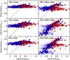 |
Fig. 5 Comparison between observed 3.6 μm–4.5 μm colour and best fit colour for a subsample of zϵ [3.8,5] objects for different models with and without nebular emission. Blue dots show objects identified as “strong” nebular emitters, and red dots are “weak” nebular emitters. |
For the subsample of objects with redshifts z ~ 3.8–5 as discussed above, the observed 3.6 μm–4.5 μm colour provides also an interesting constraint on star formation history and nebular emission. Indeed, models without nebular emission are unable to reproduce the range of observed 3.6 μm–4.5 μm colours at z ~ 4, as shown in Fig. 5. The REF+NEB model (constant star formation) is also unable to reproduce the observations, while the DEC+NEB and RIS+NEB models provide fits fully consistent with this colour (+NEB+Lyα option leads to similar results) with DEC+NEB providing even better results than RIS+NEB. Abandoning the age limitation (age >50 Myr) for the REF+NEB model would allow this model to provide fits consistent with observations. We need to have very large Hα equivalent widths to reproduce the colour of “strong” nebular emitters. This can be obtained for any SFH with young ages (median of ~ 20 Myr for DEC+NEB and RIS+NEB). On the other hand, small EW(Hα) for “weak” nebular emitters are necessary to reproduce their red colour. Since no physical process is able to suppress effectively nebular emission for both rising and constant SFs, DEC+NEB(+Lyα) is the model which best fits both LBG categories. However, RIS+NEB(+Lyα) and REF+NEB(+Lyα) also provide acceptable fits for “weak” nebular emitters, considering errors in colour estimation. Further constraints and results on the timescales of the exponentially declining star formation histories are discussed in Sect. 4.3.5.
Finally, we have found a shift between those best fit with or without Lyα (i.e. between +NEB and +NEB+Lyα option) with redshift, among objects better fit with nebular emission. In this sense the higher-z galaxies favour a larger fraction of objects with Lyα emission. This shows that SED fitting is also sensitive to Lyα emission, which is a finding we have demonstrated and discussed in detail in Schaerer et al. (2011).
4.3. Physical properties of the LBGs
We now turn to discuss the main physical properties (stellar mass, SFR, age, attenuation, and the star formation timescale where appropriate) of the LBGs and their dependence on model assumptions. The median values and uncertainties of the physical parameters derived in several bins of UV magnitude M1500 for all our samples and by using all nine combinations of model assumptions are listed in Tables A.1–A.3. For each physical parameter, we now describe the median properties and their model dependence, explain their origin, and compare the behaviour of the individual values. Furthermore, we examine possible correlations between derived and observed parameters. To do this, we choose the largest subsample, here consisting of 705 B-drop (z ~ 4) galaxies, since the same trends/differences overall are found at all redshifts (except stated otherwise). In Sect. 4.4, we then discuss the redshift evolution of the physical parameters and their model dependence.
4.3.1. Absolute UV magnitude
In what follows, the absolute UV magnitude M1500 refers to the absolute magnitude at 1500 Å. To determine it for each object, we use the integrated SED flux in an artificial filter of 200 Å width centered on 1500 Å. Using the V-band magnitude for U-drop, i-band for B-drop, and z-band for V- and i-drop samples and spectroscopic redshift when availaible to estimate the UV magnitude (Stark et al. 2009) leads to no significant difference on M1500, except for one B-drop, two V-drop, and one i-drop galaxy. These are objects with a spectroscopic redshift identification at low redshift, which passes our selection. As they represent less than 1% (slightly more for i-drop) of each sample, we consider that they can not alter significantly our conclusions. In passing, we note that the number of objects in each UV magnitude bin listed in Tables A.1–A.3 can change from one model to another, mostly due to small differences in photometric redshifts.
 |
Fig. 6 Composite probability distribution of age for REF model and age for all other models at z ~ 4. The points overlaid show the median value properties for each galaxy in the sample. Black dots represent “weak” nebular emitters and white dots “strong” nebular emitters. The overlaid contour indicates the 68% integrated probabilities on the ensemble properties measured from the centroid of the distribution. |
4.3.2. Age
Overall, the ages of individual z ~ 4 LBGs derived from the different models span a wide range, typically from ~4 Myr (if no lower limit is specified) to ~1.5 Gyr, which is the maximum age at this redshift (see Fig. 6). A wide age range is found for all nine model sets.
The individual ages and the resulting median age of the sample depend strongly on the model assumptions. As can be seen in Tables A.1–A.3 and by assuming declining (DEC) or rising (RIS) star formation histories leads for models without nebular emission to median ages younger by a factor 5–10 as compared to constant star formation (REF). These differences are much larger than the typical age uncertainty (~0.15 dex) found for the REF model. The reason is that galaxies keep a high UV rest-frame flux with a constant SF and if the observed SED shows the presence of a Balmer break, older ages are necessary for the population to reproduce the observed break. For a declining or rising SF, much younger ages are enough to obtain a suitable evolved population. Indeed, the observed median ratio of the optical/UV flux is high and consistent with a Balmer break at each redshift (see González et al. 2010; Lee et al. 2011).
The effect of different assumptions on age estimation is more easily understood if we examine the two populations, “weak” and “strong” emitters, separately as defined in Sect. 4.1. For “strong” nebular emitters, median ages are decreased for all SFHs and for all redshift, which is an expected result (Schaerer & de Barros 2009, 2010), since emission lines (mostly [O iii] λλ4959, 5007 and Hβ) can mimic a Balmer break. This effect is strong enough (e.g. by a factor 2–10 for the REF model; see Fig. 6) to lead to significant differences between models, even considering uncertainties. Uncertainties are increased when nebular emission is taken into account: from 0.15 to 0.27 dex for REF models, from 0.39 to 0.55 dex for RIS models. These increased uncertainties are due to double peaked age probability distribution functions (Schaerer & de Barros 2010), since these objects can be fit with young population (and strong lines) or old population (Balmer break). For declining SFH, there is no such effect, since there are already large uncertainties on age (~ 0.4 dex, even without nebular emission) because of the strong degeneracy between age and timescale.
For LBGs with “weak” lines, considering nebular emission leads to older ages, a result that can be easily explained if we assume that these objects have truly weak lines: the only way to decrease emission lines strength is by adopting old ages at least with our assumptions and SFHs. While the trend is the same for all SFHs, there are quantitative differences with older ages by a factor 2–5 for REF and DEC models (at z ~ 4) and a factor 10–20 for rising SF.
In absolute terms, the derived ages of “weak” and “strong” nebular emitters are fairly similar when REF models are assumed. For decreasing and rising SF, the ages of “strong” emitters are systematically decreased when considering nebular emission, while they are increased for “weak” emitters. “Strong” emitters are younger by a factor ~2 (DEC+NEB model) to ~5 (RIS+NEB model) in comparison with “weak” emitters. In any case, the age differences seem to confirm an intrinsic difference between these two LBG categories, and the strength of the lines seems to be the main driver for the age determination at high redshift when nebular emission is taken into account.
4.3.3. Reddening
The attenuation of individual z ~ 4 LBGs derived from the SED fits range from AV = 0 to a maximum of ~1.5–2 mag for a few objects, as shown in Fig. 7. Although all model sets yield a similar range of attenuation, relatively large systematic differences, which we discuss, are found between them.
Whether one considers nebular emission or not for a given SFH a variation no larger than 0.2 mag can be determined. Comparing REF model to other models (without nebular emission), the median AV is higher for the DEC model (+0.2 mag) and for the RIS model (+0.5 mag), which can be partially explained by the well known degeneracy between reddening and age, since DEC and RIS models lead to younger median ages than constant SF (cf. above). Furthermore, a higher attenuation is required to fit the observations, compared to models with constant SF, as already pointed out by Schaerer & Pelló (2005), since young stars always dominate the UV flux for rising star formation histories. Considering this, nebular emission leads to variations no larger than 0.1 mag in reddening for the REF model on average; a slight increase is found when the Lyα line is included (REF+NEB+Lyα model, assuming the maximum case B intensity for Lyα), which is explained by the additional flux from the Lyα line.
On the other hand, nebular emission leads to a systematically lower median AV for rising star formation history, since the contribution of strong nebular lines in the optical and infrared (rest-frame) leads to redder SEDs, because of extremely large EWs (see Table 2). This effect is seen for both “weak” and “strong” categories. These results have to be taken with some caution since typical errors on AV for individual objects are 0.1 mag for constant SF and ~0.2 mag for decreasing and rising SF, which does not allow a clear distinction for example between REF and DEC models.
This latter result can seem surprising since previous studies at z ~2 (e.g. Shapley et al. 2005; Erb et al. 2006b; Reddy et al. 2012b) found that a declining SFH usually leads to lower dust attenuation than a constant SFH due to the best fits with t/τ > 1. This implies that there is a significant population of old stars that explained the redness of UV continuum. This also leads to a discrepancy between the SFR inferred from the SED fitting and other SF indicators (Erb et al. 2006b; Reddy et al. 2012b) with a declining SFH which leads to an underestimated SFR. Our SED modelling results differ from these previous studies on the t/τ ratio, for which we find that 40–50% of our objects (at all redshift) have t/τ < 1. This condition should provide similar results between declining and constant SFH in terms of dust attenuation and SFR. Since we allow younger ages for DEC models than for REF models, we find typically higher dust attenuation and SFR. By comparing our SED modelling with those from Shapley et al. (2005), Erb et al. (2006b), and Reddy et al. (2012b), we find that these three studies rely only on solar metallicity, when we use three different metallicities (0.02, 0.2, and 1 Z⊙). Papovich et al. (2001) shows in their Fig. 10 that the impact of subsolar metallicity on confidence intervals for a composite probability distribution function between age and timescale. While the range of possible values is large at solar metallicity, it is increased at lower metallicity, mainly in the t/τ < 1 area. Indeed, if we consider our models with a declining SFH in our three metallicity bins, we find a trend consistent with this result: objects with t/τ < 1 are 25–30% at Z = Z⊙ up to 60–80% at Z = 0.02 Z⊙. This shows how some parameters can be sensitive to assumption on metallicity. We are remind that we infer median physical parameters of each object and sample through MC simulations with a marginalization over the parameter space. As shown in Tables A.2 and A.3, metallicity is bracketed between 0.2 and 1 Z⊙ at z ~ 3−5, which is consistent with metallicity inferred at z ~ 2 (Erb et al. 2006c). Extreme subsolar metallicity (0.02 Z⊙) is preferred only at z ~ 6. We provide full comparison with several other studies in Sect. 5.2.
 |
Fig. 8 AV distribution at z ~ 4 (DEC+NEB model) for “strong” (blue) and “weak” emitters (red). |
The inclusion of nebular emission with a constant star formation history does not lead to any significant change in dust reddening for “weak” nebular emitters. For declining and rising SF, the extinction decreases strongly (by ~−0.2 to −0.5 mag in AV) when we consider nebular emission. Since these objects seems to have intrinsically no discernible signs of emission lines, models include a nebular emission fit by minimizing equivalent widths, which is achieved by minimizing SFR and UV flux. Model sets based on constant star formation history (REF/REF+NEB/REF+NEB+Lyα models) do not allow sufficient variations to modify the reddening estimation. For “strong” nebular emitters, the median AV increases (by +0.2 to +0.5 mag) between z ~ 3 and ~5 when we consider declining star formation, while it decreases for rising SF (−0.1 to −0.2 mag), as already explained. The increased dust attenuation with DEC+NEB model can easily be explained by the effect of emission lines on age, leading generally to younger ages and thus to a bluer slope.
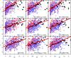 |
Fig. 9 UV-continuum slope β vs. AV for all models at z ~ 4. Each cross shows the median value properties for each galaxy: blue for “strong” nebular emitters and red for “weak” nebular emitters. Black squares are median values by bins of 0.1 AV mag. The dashed red line is the relation between extinction (Calzetti et al. 2000) and a given β if the base spectrum is a young star-forming galaxy of constant star formation (Bouwens et al. 2009). The red line is a linear fit among the whole composite probability distribution function. |
At z ~ 6, effects of modelling with nebular emission are different: for decreasing and rising model sets, the consideration of nebular emission leads to a decrease of the median AV for both “weak” and “strong” nebular emitters, respectively with ~−0.6 and ~−0.2 mag. The SED fits with nebular emission lead to an important contribution of nebular lines longward UV, and so an additional amount of dust attenuation is required, since strong lines are associated with strong UV flux.
Overall, “strong” emitters are more dusty than “weak” emitters. Figure 8 illustrates this for the DEC+NEB model, and a KS-test shows that the AV distributions are drawn from different populations if we consider any model that accounts for nebular emission (at z ~ 4, p < 10-5), even REF+NEB model (constant SF and age >50 Myr). In contrast, p = 0.72 for the REF model.
4.3.4. Reddening and UV-slope
Since the observed UV slope β is often used to measure the attenuation in
LBGs, it is interesting to examine how the attenuation derived from the SED fits are
based on the different model assumptions that compare with β. Such a comparison is
shown in Fig. 9 for the nine model sets applied to
the B-drop
sample. The UV slope has been determined using the same filters and relations as Bouwens et al. (2009). Figure 9 shows that there is a significant trend of increasing
β with
AV, as expected,
albeit with a large scatter for individual objects. We have done linear fits to the 2D
composite probability distribution function, which yields the mean relations indicated
in the plot by red lines. For comparison, the “standard” relation between
β and
AV taken here from
Bouwens et al. (2009) is also shown. As
expected, our relations agree well with the “standard” one for models assuming constant
star formation and ages >50 Myr (REF model sets), since this
corresponds to the main assumptions made to derive the standard β-reddening relation. For
a given SF history, differences between the three options with/without nebular emission
can be explained by the behaviour of AV discussed above.
Since all models with declining and rising star formation histories yield higher
reddening on average (cf. above), a relation shallower than the standard one is found.
Since the relations obtained are fairly similar, we can combine them to obtain the
following mean relations between β and AV for the three
cases: (1) modeling without nebular
emission; (2) +NEB+Lyα; and (3) +NEB. This is shown as 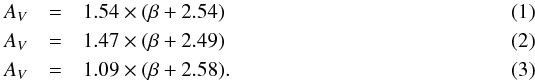 The
last relation (Eq. (3)) is probably the
most appropriate one, since it combines the models which best fit the data (i.e. models
including nebular emission but no strong Lyα for the majority of the galaxies, cf. Schaerer et al. 2011). It should be reminded that
these relations assume a Calzetti attenuation law. To translate this into the colour
excess one has E(B − V) = AV/RV,
where RV = 4.05. In
short, we find that LBGs with a given UV slope have higher attenuation than derived from
the commonly used β–AV relation, from our
new relations derived from a subsample of 705 B-drop galaxies using various star formation
histories. For typical UV slopes of β ~ −2.2 (−1.7) found for faint (bright)
z ~ 4
galaxies, this translates to an increase in the UV attenuation by a factor
~3.
The
last relation (Eq. (3)) is probably the
most appropriate one, since it combines the models which best fit the data (i.e. models
including nebular emission but no strong Lyα for the majority of the galaxies, cf. Schaerer et al. 2011). It should be reminded that
these relations assume a Calzetti attenuation law. To translate this into the colour
excess one has E(B − V) = AV/RV,
where RV = 4.05. In
short, we find that LBGs with a given UV slope have higher attenuation than derived from
the commonly used β–AV relation, from our
new relations derived from a subsample of 705 B-drop galaxies using various star formation
histories. For typical UV slopes of β ~ −2.2 (−1.7) found for faint (bright)
z ~ 4
galaxies, this translates to an increase in the UV attenuation by a factor
~3.
While implications of our different reddening estimation are discussed in Schaerer et al. (2013), we note that our preferred β-AV relation differs from the one found at z ~ 2−3 with radio, X-ray and IR data (Reddy & Steidel 2004; Reddy et al. 2010, 2012a), which is consistent with the β-AV relation established by Meurer et al. (1999). However, this relation relies on several assumptions, such as β0 (UV continuum slope in the absence of dust absorbtion) being dependent from the SFH, metallicity, and IMF (Leitherer & Heckman 1995). The value of β0 = −2.23 is obtained with a constant SFH lasting for 100 Myr, solar metallicity, and a Salpeter IMF. Since we obtain significant fractions of galaxies that have an age <100 Myr, and subsolar metallicities, we find β0 ~ −2.6, which is a value consistent with prediction from Leitherer & Heckman (1995) under similar assumptions.
 |
Fig. 10 Theoretical SEDs in the rest-frame, which are normalized at 2000 Å for models with EW(Hα) = 500 Å (solid lines) and 100 Å (dashed lines) and different star formation timescales (constant SF in red and τ = 10 Myr in blue). For the models with EW(Hα) = 500 Å, the ages are 52 Myr and 16 Myr respectively. For EW(Hα) = 100 Å, 2.1 Gyr and 35 Myr. |
 |
Fig. 11 Evolution of EW(Hα) (blue), and z850LP − 4.5 μm colour (red) with age for τ = 10 Myr (solid lines) and for τ = ∞ (dashed lines). Typical error bars, as shown on the left for EW(Hα) and on the right for the z850LP − 4.5 μm colour, have been derived from error estimation on measured fluxes at z ~ 4. The effect of redddening (AV = 0.5) on z850LP − 4.5 μm is shown with the red arrow. |
 |
Fig. 12 z850LP − 4.5 μm observed colour histogram at z ~ 4. In red, we have best fit objects with τ ≥ 100 Myr, and in blue, best fit objects with τ = 10 Myr for the three models with decreasing SF. The dashed blue, red, and black lines show respectively a median colour for objects that are best fit with τ = 10 Myr, with τ ≥ 100 Myr and for the whole sample. For the two subsamples, KS test for the three models gives p = 7.8 × 10⁻⁸, p = 2.6 × 10⁻¹⁷, and p = 1.3 × 10⁻¹⁶, respectively, for DEC, DEC+NEB+Lyα, and DEC+NEB models, showing that the two subsamples are not drawn from the same population. |
4.3.5. Star formation timescale
For the models with exponentially declining star formation histories (DEC models),
which are found to provide the best fits for the majority of objects (i.e. lower
) but not
always by large margins it is of interest to examine the resulting timescales
τ and the
uncertainties on this quantity. As a reminder, the DEC model set considers 10 different
star formation timescales τ ∈ [10,3000] Myr plus the
limiting case of τ = ∞ that corresponds to constant star formation.
For all options with/without nebular emission (DEC, DEC+NEB+Lyα and DEC+NEB), we find
median values of τ between 10 and 300 Myr in the different UV
magnitude bins (cf. Table A.2). Models including
nebular emission favour shorter timescales on average than those without. Although the
timescales found are relatively short compared to the dynamical timescale at values of
 Myr at z ~ 4 (Bouwens et
al. 2004; Ferguson et al. 2004; Douglas et al. 2010; Förster Schreiber et al. 2009) the uncertainties on τ are large.
Myr at z ~ 4 (Bouwens et
al. 2004; Ferguson et al. 2004; Douglas et al. 2010; Förster Schreiber et al. 2009) the uncertainties on τ are large.
What constrains the SF timescales and why are short timescales preferred? Since SFR ∝ exp(−t/τ), two (or more) observational constraints are needed to determine both the age t and timescale τ. Lets us first consider the case of models that include nebular emission and examine galaxies with z ~ 3.8−5. In this case, we find that t and τ are mostly constrained by a combination of the (3.6−4.5) μm colour tracing EW(Hα) and by a UV/optical (rest-frame) colour. This works as follows. As already discussed above, the 3.6−4.5 μm colour of galaxies at z ~ 3.8–5 reflects the Hα equivalent width. However, it is well known that a given equivalent width can be obtained with different values of t/τ (cf. Fig. 11). To illustrate this, we show the predicted SEDs for galaxies with the same EW(Hα) = 100 (500) Å but different SF timescales (τ = 10 Myr and ∞) in Fig. 10. It is obvious that the main feature allowing to lift this degeneracy is the ratio of the UV/optical flux. At z ~ 4, this ratio is reflected by the z850LP − 4.5 μm colour, whose evolution with t and τ is also shown in Fig. 11. Therefore, these two colours provide good constraints on t and τ, assuming they are not strongly affected by reddening (cf. below). Within the typical 68% error bars, these two extreme SFHs can be discriminated by their colour and EW(Hα) for t ≳ 20–30 Myr. For younger ages, the uncertainties in both EW(Hα) and colour do not allow a clear separation. A posteriori, we can verify that the objects best fit with “long” timescales do indeed statistically differ from those with “short” timescales. Figure 12 shows a statistically significant difference between galaxies best fit with τ = 10 Myr, which are bluer in z850LP − 4.5 μm and τ > 100 Myr galaxies showing redder colours.
We also have to consider dust attenuation, which can increase z850LP − 4.5 μm, as shown in Fig. 11, and introduce a degeneracy between SFHs. However, considering the observed median colour and dust attenuation for the REF and DEC model sets, we expect to have higher extinction for REF model sets than for DEC model sets, but we find the opposite with a median AV that is larger by 0.1–0.2 mag for DEC models. Furthermore, Fig. 11 shows that it is more difficult to reproduce a given red colour with a constant SF than with a declining SF. This shows that dust attenuation seems to be only weakly correlated with z850LP − 4.5 μm colour at z ~ 4, which allows us to conclude that the ratio of UV/near-IR flux and equivalent widths of different emission lines (mainly Lyα, Oiii and Hα) drive the choice of τ for models with declining star formation. Despite the possibility to discriminate two extreme SFHs like constant SF and decreasing SF with τ = 10 Myr, large uncertainties on τ estimates are found (from 0.7 dex for DEC+NEB+Lyα model to ~2 dex for DEC+NEB model), which prevents us to derive strong constraints on τ. These uncertainties come mainly from reddening; indeed, fixing reddening to an arbitrary value (AV = 0) also lead to a low median τ (<300 Myr) but with lower typical uncertainties from ~0.4 dex for the DEC+NEB+Lyα model to ~0.6 dex for the DEC model.
Interestingly, our models with declining SF histories indicate a possible increase of the timescale τ with UV luminosity also with stellar mass but only for “strong” nebular emitters. It is tempting to suggest that this could be due to a decrease of the feedback efficiency with increasing galaxy mass, since the star formation timescale is likely related to the dynamical one and modulated by feedback (e.g. Wyithe & Loeb 2011). We do not see any evolution of the timescale for the “weak” nebular emitters, which is easily explained by weaker constraints due to the absence of strong distinctive features. This explains why the trend of τ with UV magnitude cannot be seen in Table A.2, where the combined data for the entire sample is listed.
4.3.6. Stellar mass
Stellar mass is generally considered as the most reliable parameter that is estimated by SED fitting, since relatively small differences are found when varying assumptions like the star formation history or dust extinction. Finlator et al. (2007) estimates that differences due to different assumptions on SFHs are typically not higher than 0.3 dex, and Yabe et al. (2009) who adds effects of metallicity and extinction law, estimates differences to be not higher than ~0.6 dex. Our stellar mass comparisons based on different model assumptions are shown in Fig. 13 and in Tables A.1–A.3. Our results confirm the earlier results about the stellar mass dependence on the assumed SFH. Indeed, median stellar masses do not differ by more than ~0.3 dex among different star formation histories from z ~ 3 to z ~ 6, when we do not account for nebular emission, even using metallicity as a free parameter. With respect to models with constant star formation and without nebular emission (REF), all other models and options (+NEB or +NEB+Lyα) lead systematically to lower stellar masses with differences larger than the typical uncertainty of ~0.15 dex found with the REF model. The REF+NEB/+NEB+Lyα models (constant SF, nebular emission and age >50 Myr) lead to stellar mass differences of the same order as typical uncertainty, not larger than ~0.2 dex. For DEC and RIS models and the accounted nebular emission, we find stellar masses that are lower by ~0.4 dex on average compared with REF model.
Differences in stellar mass found between “strong” and “weak” emitters are again consistent with an intrinsic difference between these two categories. When we consider nebular emission, stellar mass estimation of “strong” emitters are more affected than for “weak” emitters. Typically, stellar masses decrease by ~0.4–0.9 (0.2) dex for “strong” (“weak”) nebular emitters in comparison to stellar mass estimates from the REF model. Furthermore, when we account for nebular emission, “strong” emitters are slightly less massive than “weak” emitters for any SFH (~0.1 dex), while both categories overall span the same range of stellar mass and MUV.
This is due to the less extended range of possible EW, since the impact of nebular emission on stellar mass estimation is correlated with this quantity. Indeed, as shown in Fig. 11, declining SFH allows EW(Hα) variations up to 3 dex, while our REF+NEB+Lyα/+NEB model shows possible variation of EW(Hα) by a factor ~5. For these latter models, contribution of emission lines to broadband photometry is roughly similar for any objects, and thus, by considering nebular emission, does not introduce large variation on stellar mass estimation.
 |
Fig. 14 Composite probability distribution of M1500 and M⋆ for all the models at z ~ 4. The dashed black line represents the M⋆–M1500 trend found by González et al. (2011), and the dotted black lines show a scatter of ±0.5 dex. The solid red line shows a linear fit established by considering the whole composite probability distribution. The points overlaid show the median value properties for each object in the sample, black dots for “weak” nebular emitters and white dots for “strong” nebular emitters. The overlaid contour indicates the 68% integrated probabilities on the ensemble properties measured from the centroid of the distribution. |
 |
Fig. 15 Composite probability distribution of M⋆ and age at z ~ 4. The points overlaid show the median value properties for each object in the sample, black dots for “weak” nebular emitters and white dots for “strong” nebular emitters. The overlaid contour indicates the 68% integrated probabilities on the ensemble properties measured from the centroid of the distribution. |
In Fig. 14, we show the stellar mass–M1500 relation found for all our models at z ~ 4. For constant star formation with or without nebular emission, we find, as expected, a relation in good agreement with the one found in González et al. (2011) within a scatter of ±0.5 dex. Indeed, our REF model is based on assumptions similar to those of González et al. (2011), except for the metallicity (We assume Z = Z⊙ when they assume Z = 0.2 Z⊙.) and for the minimum age (We assume 50 Myr when they assume 10 Myr.) Considering that the solar metallicity leads to ~0.06 dex of increase in mass in comparison with 0.2 Z⊙ and a higher minimal age increasing the lower bound in M⋆, the slight offset of our stellar mass–M1500 Å relation is easily explained. Although differences exist in the M⋆–M1500 relation obtained among different model sets, our relation remains overall (within the scatter of ± 0.5 dex) fairly similar to the relation derived in González et al. (2011).
A correlation between stellar mass and age is found for all the models, as shown in Fig. 15. Since age estimation depends on the mass to light ratio, this relation is trivial if we describe the star formation history with a monotonic function. Indeed, luminosity is fixed by both measured fluxes and redshift, and the near-IR data putting strong constrains on the stellar mass estimation. The stellar mass-age relation simply reflects the increase in the mass to light ratio with age. As previously explained, different assumptions on the SFH lead to different trends between “weak” and “strong” nebular emitters when analysed with SEDs that include nebular emission: for variable star formation histories (both rising or declining) “weak” nebular emitters are found to be older and more massive on average than “strong” nebular emitters. In contrast, physical properties of the two populations do not differ when constant star formation and an age >50 Myr is assumed (REF model).
In Fig. 16, we show the relation between the dust attenuation AV and stellar mass for a selected model set. For all models, a similar trend is found with the median AV which increases with galaxy mass, and a wide range of attenuations that are allowed between 0 and ~1.5 mag. Figure 17 helps to understand the correlation between stellar mass and dust reddening, since it shows that the dispersion comes mainly from age scatter. Indeed, we find a clear trend of increasing extinction with increasing stellar mass for a given range of age. This trend has already been highlighted at lower redshifts (eg. Buat et al. 2005, 2008; Burgarella et al. 2007; Daddi et al. 2007; Reddy et al. 2006, 2008; Sawicki 2012; Domínguez et al. 2013), and it also seems to be observed at higher redshift (Yabe et al. 2009; Bouwens et al. 2009; Schaerer & de Barros 2010). This is clearly compatible with our results but with large uncertainties. While this trend could be explained by the age-reddening degeneracy, fixing age at a given value leads to no change. The most likely natural explanation of this trend is probably that the dust attenuation is related to the stellar mass-metallicity relation (cf. Tremonti et al. 2004; Erb et al. 2006a; Finlator et al. 2007; Maiolino et al. 2008).
 |
Fig. 17 Relation between stellar mass and reddening for DEC+NEB model at z ~ 4. Blue dots represent galaxies with median age ≤ 107 years; red squares: 107 < age ≤ 108, yellow upward triangles: 108 < age ≤ 109 and black downward triangles: age >109 years. |
 |
Fig. 19 Distribution of the ratio t/τ at z ~ 4, with objects with age ≤50 Myr in blue, and objects with age >50 Myr in red. |
4.3.7. Star formation rate
The star formation rate (defined here as the instantaneous value at the age t) depends strongly on the model assumptions, as illustrated in Fig. 18. For the REF model (constant SF and age >50 Myr), the inclusion of nebular emission leads to higher SFRs on average due to the younger age, which requires a higher attenuation. The largest differences (up to ~1 dex) with respect to constant SFR models are obtained with DEC models. The reason for such differences is obviously due to the variations in the UV output with time and young ages (<50 Myr), which also imply a higher attenuation on average (cf. above).
An interesting feature of the declining SF histories is that it also allows for SFRs which are lower than those derived using the canonical calibrations, assuming constant SFR. Typically, galaxies with t/τ ≲ 1 have higher SFR (up to 1 dex), if the timescale is short enough to diverge significantly from REF models. The range of τ values in our sample is given in Table A.2, while Fig. 19 shows the range of ratio t/τ for the DEC model at z ~ 4. Galaxies with t/τ ≳ 2 are more quiescent1 and have lower SFR (up to 1 dex). Lastly, intermediate galaxies have SFRs that are consistent with results from the REF model. This larger “dynamic range” may well be physical, as indicated by the existence of “strong” and “weak” nebular emitters, as we discuss below. Models with rising star formation histories lead to the highest SFRs, since their SED is always dominated by young stars. This implies a narrower range of UV-to-optical fluxes, hence requiring a higher attenuation on average than for other SF histories (cf. above, Schaerer & Pelló 2005). For rising SF with ages above ~108 yr, all galaxies follow the canonical relation (Kennicutt 1998). Below this age, the SFR estimated by SED fitting is higher for the same reason as for decreasing SF (regardless of dust reddening).
 |
Fig. 20 Same as Fig. 15 for M⋆ and SFR. The dashed line represents the SFR–M⋆ relation found in Daddi et al. (2007) at z ~ 2. |
We determine that nebular emission does not lead to any significant changes in the median SFR for the REF model, while the median SFRs are lower for decreasing SF (mainly for +NEB+Lyα) or equal (mainly for +NEB). For rising SF, the median SFRs are systematically lower, typically by a factor ~2. From z ~ 3 to 5, this effect is due to the difference in dust reddening and age estimations, and to the contribution from Lyα line in the case of +NEB+Lyα due, which can decrease the UV flux necessary to fit the measured fluxes.
Relying on our previous identification of “strong” nebular emitters and “weak” nebular emitters (Sect. 4.1), we are able to check the consistency of star formation rate estimation. Since emission lines are produced by the strong UV flux from OB stars in H ii regions, we should find a higher SFR for “strong” nebular emitters in comparison with “weak” nebular emitters, for a given stellar mass. As shown in Fig. 18, the REF model does not reproduce such a separation between “strong” and “weak” emitters, since SFRs are roughly similar for both populations or even showing an opposite trend to what is expected. The inclusion of nebular emission in the REF model does not lead to a significant difference on median SFR estimations between the two populations. Other models without nebular emission (DEC and RIS) do not provide a better result than the REF model, since they also provide an opposite trend to what is expected – a higher median SFR at a given stellar mass for “weak” nebular emitters. On the other hand, the two populations are naturally separated in terms of SFR, as shown in Fig. 18 when nebular emission is included. This reveals the “strong” nebular emitters as objects with a strong ongoing star formation episode, and “weak” emitters as a more quiescent population. The capacity of both the declining and rising star formation histories to distinguish these populations can be easily understood, since young ages (<50 Myr) lead to deviate from the canonical UV to SFR relation (Reddy et al. 2012b). Separating the two LBG populations, we find that the median SFR is higher by ~0.6 dex (up to 0.75) for the “strong” nebular emitters from z ~ 3 to z ~ 5 compared to the “weak” emitters, although the typical uncertainty is relatively large (~0.5 dex). Since the stellar mass is not significantly different between “weak” and “strong” emitters, the specific SFR (SFR/M⋆) of the “strong” is higher than that of the “weak”. At z ~ 6, only DEC/RIS+NEB+Lyα models lead to the expected trend (separation between “weak” and “strong” emitters in term of SFR–M⋆ relation), showing that the presence of just one emission line, such as Lyα can have a large impact on parameter estimation (Schaerer et al. 2011).
We now explore the SFR–M1500 relation, as illustrated in Fig. 22 for the z ~ 4 sample using three different models sets. For the constant star formation (REF) model, the SFR–M1500 match with the Kennicutt calibration (Kennicutt 1998), once accounting for the effect of dust extinction. As explained in Kennicutt (1998), the relation is valid for galaxies with continuous star formation over time scales of 108 years. The SFR/L1500 will be significantly higher in bursty galaxies with a decreasing SF and a short timescale, or for simply galaxies younger than 108 years (cf. Reddy et al. 2012b; Schaerer et al. 2013). This leads to significantly higher SFR than those given by the Kennicutt relation, regardless of dust reddening. The SFRs found cover a large range of possible values, which strongly depend on both SFH and whether they fit or not with nebular emission (see Table A.1–A.3). Again, only rising and declining SF with nebular emission are able to separate the two populations previously identified as “strong” and “weak” nebular emitters, since they naturally separate these groups into higher and lower SFR galaxies at a given MUV.
The SFR as a function M⋆ is plotted in Fig. 20 for the z ~ 4 sample. The figure shows that we find a relation compatible to that found at z ~ 2 by Daddi et al. (2007) with a relatively small dispersion, and no significant difference if we consider nebular emission for constant star formation (REF model). For decreasing SF, our results remain compatible with the relation at z ~ 2 but with a very large dispersion, which can be explained by the large range of timescale. For rising SF, the star formation rates are systematically higher than those expected from the SFR–mass relation derived at z ~ 2. For rising and decreasing star formation, we note that the galaxies seem to be separated in two groups: actively star forming galaxies, showing higher SFRs than expected from the Daddi et al. (2007) relation, and a group of more quiescent galaxies, which are compatible with this relation. These groups correspond again to those previously identified as “weak” and “strong” nebular emitters.
The specific star formation rate (sSFR = SFR/M⋆) is plotted for z ~ 4 as function of stellar mass in Fig. 21. For all models, it decreases on average with increasing M⋆ and with decreasing redshift. The relation is fairly similar among all models but decreasing and rising star formation histories lead to higher sSFR values by more than 1 dex. This increase is significant compared to the typical errors, which range from ~0.2 dex for models with constant SF to ~0.6 for decreasing and rising SFHs. For decreasing and rising SF, the presence of Lyα leads to a slightly lower SFR and a higher M⋆ (except at z ~ 6 where this trend is reversed), which explains the lower sSFR when compared to models that assume no Lyα emission. By comparing declining star formation histories to others, we find that they yield lower sSFR for some galaxies. With both the DEC+NEB(+Lyα) and RIS+NEB(+Lyα) models, “strong” nebular emitters have a slightly lower median M⋆, and a higher SFR than the “weak” nebular emitters. In other words, we find that “strong” emitters show a higher sSFR than “weak” nebular emitters at a given mass.
4.3.8. Metallicity
Metallicity is the least constrained parameter by our SED fits. For individual objects the 68% confidence interval for all samples basically covers the three metallicity values (0.02, 0.2, 1 Z⊙) used here. Considering the median metallicity, there is a trend for RIS+NEB(+Lyα) and DEC+NEB(+Lyα) models to show an increase in the metallicity with galaxy mass. However, the uncertainties are too large to provide firm conclusions. This is consistent with the well known fact that metallicity is poorly constrained by SED fitting.
4.3.9. Physical properties: summary
Accounting for nebular emission in the SED fitting decreases the estimated age in most cases2, since some strong lines can mimic a Balmer break, increase dust attenuation, and decrease stellar mass, as already found earlier (Schaerer & de Barros 2009, 2010). The extent of this impact strongly depends on assumptions on both star formation history and the allowed age range. An increasing SFH produces strong lines at any age, while constant and declining SFHs lead to a decreasing impact of emission lines with age (Fig. 11). We find that young ages (<50 Myr) are required to reproduce the most extreme observed (3.6−4.5) μm colours of Fig. 5, which corresponds to strong Hα emission at zϵ [3.8,5] (Shim et al. 2011). Only DEC+NEB and RIS+NEB models are able to reproduce these colours.
 |
Fig. 22 Composite probability distribution of M1500 and SFR for the REF (top), DEC+NEB (centre) and RIS+NEB model (bottom) for the sample at z ~ 4 as determined for each galaxy from our 1000 Monte Carlo simulations. The overlaid points show the median value properties for each object in the sample with black dots for “weak” nebular emitters and white dots for “strong” nebular emitters. The overlaid contours indicate the 68% integrated probabilities on the ensemble properties measured from the centroid of the distribution. The dashed line represents the Kennicutt relation (Kennicutt 1998). |
 |
Fig. 23 Median ages are given in bin of absolute magnitude at 1500 Å (no correction for dust) from z ~ 3 to 6 for four models. Squares illustrate constant SFR with downward (upward) triangles decreasing (rising) SFHs. Black symbols stand for models without nebular emission; red symbols for models that include nebular emission (NEB), and blue symbols for NEB+Lyα. The error bars correspond to the 68% confidence limits of the probability distribution in each bin. Dashed lines show the amount of time spanned, since the previous redshift bin. |
From the best fit distribution (Sect. 4.2), we identified two LBG populations, one which seems to show stronger nebular emission than the other, defined as “strong” and “weak” emitters (respectively). Using DEC+NEB and RIS+NEB models, this latter population is slightly more massive, less attenuated, and older than “strong” emitters and also exhibits lower SFR for a given stellar mass, where the parameters are compatible with a more evolved population. While differences between these two populations are less important with REF+NEB model, it is still possible to statistically distinguish these two populations (e.g. Sect. 4.3.3).
Differences in attenuation naturally lead to a difference in SFR estimation, and a significant fraction of “strong” emitters shows extremely young ages (<50 Myr), which leads to deviation from the SFR–UV standard relation (Kennicutt 1998; Madau et al. 1998).
4.4. Evolution of the physical properties from z ~ 3 to z ~ 6
We now examine the evolution of the median physical properties with redshift and discuss several implications. To allow a meaningful comparison that avoids variations of the completeness limit and the galaxy luminosity function with z, we make comparisons in bins of absolute UV magnitude. To discuss the physical parameters derived from the models that include nebular emission, we choose the models with the Lyα flux set to zero (+NEB option) for z ~ 3–5, and the NEB+Lyα option with maximum Lyα emission for z ~ 6. Within the options discussed in this paper, this choice best describes the trend of increasing strength of Lyα with redshift as observed from spectroscopic surveys (e.g. Ando et al. 2006; Ouchi et al. 2008; Stark et al. 2010), other studies (Blanc et al. 2011; Hayes et al. 2011), and our models that allow for varying Lyα strength (Schaerer et al. 2011).
In the following, we notice that there is a very small number of objects in the brightest bin at each redshift, while we plot parameters as a function of M1500, in bins of magnitude. The faintest bin falls beyond the completeness limit. It is therefore more appropriate to mainly consider the three intermediate bins to examine trends of the physical properties with UV magnitude.
4.4.1. Age
The evolution of median ages with z is shown in Fig. 23. The median age increases with decreasing redshift for the four models, typically by one order of magnitude, with no significant trend with MUV. Although declining and rising SFs lead to very similar ages at the highest redshift, they start to diverge with decreasing redshift. We found that the age differences are essentially driven by the group of quiescent galaxies with “weak” nebular emission. This is explained by both nebular emission and the intrinsically aging population with decreasing redshift. Quiescent galaxies with declining star formation prefer systematically short timescales τ (median at 10 Myr at each redshift) because the SED fitting minimize the contribution of nebular emission, which is achieved with ages significantly older than τ (at least t/τ ≳ 2), and produce a significant Balmer break. On the other hand, the only way to minimize the contribution of nebular emission for rising SF (i.e. minimize the equivalent widths of lines) is by choosing relatively old ages. Therefore, fitting SEDs that are both devoid of strong emission lines and with a strong Balmer break requires older ages than for DEC models.
Except for the model with constant SFR and no nebular emission (REF), Fig. 23 leads one to conclude that the bulk of the LBG populations at each redshift are dominated by young galaxies that were not present or visible at the previous redshift. For a constant (REF+NEB) and rising (RIS+NEB) star formation, these results imply that an important number of galaxies formed in the interval from one redshift to another, in ~300–400 Myr. For decreasing star formation, we can interpret this result with a scenario with episodes of active star formation which are followed by more quiescent episodes, because of the presence of actively star-forming and quiescent galaxies. In this scenario, age becomes a poorly constrained parameter since the underlying older stellar population, which is formed in previous episodes of strong activity, can be dominated by a newly emerged population. Obviously, the absolute ages also depend on the SF timescale. For example, fixing the timescale to τ = 100 (300) Myr for the DEC+NEB models leads to no significant differences on the median values of the stellar mass, SFR, or reddening, whereas the median age increases by a factor ~ 2 (3) for both active and quiescent galaxies.
4.4.2. Reddening
As shown in Fig. 24, the median dust attenuation decreases with increasing redshift for all the four models considered here. Inclusion of nebular emission for a constant star formation does not provide a significant difference, while decreasing and rising star formation histories lead to +0.1–0.2 and +0.3–0.4 mag respectively in reddening compared to constant SFR. Many studies (eg. Bouwens et al. 2009; Castellano et al. 2012) have shown that there is a trend of decreasing β with increasing absolute UV magnitude, which corresponds to a similar trend on M1500 − AV, which is not seen in Fig. 24. This trend should be found for the actual β − AV relation, since both the classical relation (Bouwens et al. 2009) and the relation found at z ~ 4 in this study (Sect. 4.3.4) cannot change the sign of the slope. We attempt to retrieve this trend with our different models by fitting the entire composite probability distribution function AV–M1500. However, no model among the nine considered here has been able to reproduce the expected slope, while the β–M1500 relation obtained for our z ~ 4 sample is consistent with previous studies (eg. Bouwens et al. 2009). Important degeneracies and a high dispersion for each individual object can explain this effect.
As already mentioned in Sect. 4.3.4, the median UV attenuation obtained from our models with rising and declining star formation histories and nebular emission is higher than predicted from conventional methods that rely on the average UV slope. For all models, reddening evolves similarly with redshift: it increases with decreasing redshift.
Unfortunately, while photometry in the filters commonly used to determine β (Bouwens et al. 2012) is available for the whole sample at z ~ 4, this is not the case at z ~ 5 and 6, where less than 20% of the necessary fluxes are available for the V- and i-drop samples. To circumvent this shortcoming, we use the fluxes predicted by the best fit model in these filters. At z ~ 5, we also find a deviation from the classical AV–β relation by using the equations of Bouwens et al. (2012) to derive β, although it is less important than at z ~ 4, which is an intermediate relation between the classical relation and the one we found at z ~ 4. The result is consistent with Eqs. (1)–(3) at z ~ 6, but does not allow us to distinguish among them since they are very similar at low AV, and there are only few objects at z ~ 6 with a significantly high extinction. We have to notice that we use a J-band from VLT/ISAAC, while Bouwens et al. (2012) use data from Hubble/WFC3, which can lead to some differences for the z ~ 6 objects.
 |
Fig. 25 Same as Fig. 23 for SFR and for active galaxies (i.e. “strong” emitters). The dashed line shows the Kennicutt relation (Kennicutt 1998). |
 |
Fig. 26 Same as Fig. 23 for SFR and for quiescent galaxies (i.e. “weak” emitters). The dashed line shows the Kennicutt relation. |
4.4.3. Star-formation rate
The behaviour of the instantaneous SFR as a function of the UV magnitude and for all redshifts is shown in Figs. 25 and 26, where we have separated the sample in the two groups, LBGs with “strong” and “weak” nebular emission (also referred to as “active” and “quiescent” galaxies here), as identified earlier. As previously stated, only DEC+NEB and RIS+NEB models are able to provide a consistent separation between these two populations in terms of SFR–M⋆ relation (see Sect. 4.3.7). While there is a large dispersion for individual objects, the median sSFR of “strong” emitters at each redshift is larger by ≥1 dex (≥2 dex) for DEC+NEB (RIS+NEB) models compared to REF models, whereas smaller differences (<1 or <2 dex, respectively) are found for “weak” emitters. For each group, we do not observe a significant change of the SFR with redshifts. The SFR–MUV relation does not evolve with redshift, since the median age increases with decreasing redshift, while median reddening decreases, so the two effects cancel out on average.
Figures 25 and 26 clearly show the difference between “active” and “weak” emitters in terms of SFR: “weak” emitters follow the Kennicutt relation for any model, while “strong” emitters deviate from this relation for DEC+NEB and RIS+NEB models. This can be explained by a higher dust attenuation (since we use uncorrected M1500) and/or by younger age (<50 Myr). While RIS+NEB leads to significant higher dust attenuation, differences in dust attenuation between models with constant SF and declining SF are not large (Sect. 4.3.3). Therefore, only young ages can explain the observed discrepancy between SFR(SED) and the Kennicutt relation. As shown in Sect. 4.1, these young ages are correlated with objects showing strong Hα emission at z ~ 4.
In the next section, we discuss some implications from these results on the star formation history.
4.4.4. Stellar mass and implications for star formation history
Stark et al. (2009) suggest the exploration of the star formation history of LBGs through the evolution of the stellar mass in bins of UV magnitude, since the (observed/uncorrected) UV magnitude is the most reliable tool at a high redshift to track star formation, and since stellar mass is the most reliable parameter, because it is the least dependent on different assumptions (SFH, metallicity, dust, Finlator et al. 2007; Yabe et al. 2009). While this study challenges this last assumption (Section 4.3.6), the M⋆–M1500 relation remains a useful tool to test/falsify some scenarios, specifically constant star formation history. As explained in Stark et al. (2009), if the bulk of galaxies formed stars with a constant star formation rate over sufficiently long time, we would expect to see a systematic increase in the normalisation of the M⋆–M1500 relation with cosmic time, and so with decreasing redshift. If no such change is observed, the SFR cannot be constant, at least not for more than Δt ≳ 300–400 Myr, which is the time corresponding to Δz ≈ 1 between our samples. In other words, a non-evolution of the M⋆–M1500 relation with redshift would require other star formation histories or the repeated emergence of new galaxies dominating the LBG population at each redshift.
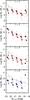 |
Fig. 27 Same as Fig. 23 for stellar mass. In each panel, we plot the M⋆–M1500 found at z ~ 4 for a more convenient comparison with other studies (Stark et al. 2009; Lee et al. 2011). Solid black line: relationship for REF model, dashed black line: REF+NEB model, dashed red line: DEC+NEB, and dash-dotted red line: RIS+NEB. |
The predicted relation between mass and UV magnitude, as obtained from all model sets and for all redshifts, is shown in Fig. 27. Although the absolute stellar masses depend on the model assumptions, all models yield essentially no evolution of the M⋆–M1500 relation between z ~ 5 to 3, but some shift between z ~ 6 and 5. In particular, models from redshift 5 to 3 with constant star formation (both with or without nebular emission, i.e. REF+NEB or REF) do not yield an evolution of stellar mass, which is inconsistent with the assumption of constant SFR. By considering the median ages obtained from the fits (Fig. 23), it seems difficult to reconcile the picture of constant star formation with the derived parameters. In contrast, the evolution of M⋆–M1500 from z ~ 6 to 5 for the REF model is fully compatible with what is expected from a constant star formation, while we still do not see the expected evolution for the same model with nebular emission. However, median ages for this latter case allow us to assume that young LBGs dominate samples at each redshift. We conclude that constant SF over long timescales is not compatible with the data.
Assuming a constant star formation and no strong evolution of the dust contain or its geometric distribution with cosmic time, we expect galaxies to evolve at constant MUV. Assuming this SFH, the evolution of UV luminosity function should be mainly due to the emergence of new galaxies (if we do not consider the effects of possible mergers). For MUV = −20.5, the number of galaxies per Mpc3 increases by a factor ~3 between z ~ 6 and z ~ 4 (Bouwens et al. 2007), which means that at least one third of the LBGs seen at z ~ 4 must have LBGs at z ~ 6 as progenitors at this magnitude. Indeed, our sample shows one third of the LBGs having an age >700 Myr at z ~ 4 and for MUV ≃ −20.5 for REF+NEB model, which correspond to the time spans between z ~ 6 to z ~ 4. We predict the median stellar mass of these galaxies at z ~ 4, using our parameter estimation at z ~ 6: the median stellar mass should be ≃ 1010.11M⊙, while our sample of galaxies at z ~ 4 that are sufficently older to be the descendants of z ~ 6 galaxies have a median stellar mass ≃ 109.55. This difference of ~0.6 dex is three times larger than the typical uncertainty on stellar mass estimation with REF+NEB model, leading us to conclude that despite a better consistency of the data with constant SF, when accounting for nebular emission, there is still significant discrepancies.
What about the rising star formation history adopted here? It is straightforward to compute how the stellar mass and SFR of each galaxy evolves with time, both forward and backward. Starting from the best fit of the 1000 MC simulations for each object, we determine how they would evolve in the future. Taking, for example LBGs at z ~ 5, which have a median stellar mass of 108.9M⊙ and a median SFR ~ 30M⊙ yr-1, we find that they would have a median stellar mass of 1011.4M⊙ and median SFR ~ 2000M⊙ yr-1 (corresponding to MUV ≃ −26 assuming the Kennicutt relation) after ~400 Myr at z ~ 4. Obviously, such extreme objects are not seen, certainly not in large numbers! To hide most of them from the LBG selection, a strong increase in dust attenuation with time would be necessary, and in this case, it should be fairly easy to find this large populations as IR/sub-mm galaxies. More likely, this discrepancy implies that the average rising star formation history adopted from the simulations of Finlator et al. (2011) are not representative for typical z ≲ 6 galaxies: that is, the growth does not continue significantly beyond the current ages of the LBGs, or the growth is too fast, or that a combination of these arguments apply3. In any case, the study of Papovich et al. (2011) shows that to have an observed number counts at z ~ 3–8 compatible with a cosmologically average rising star formation history, the growth of the SFR has to be fairly slow. Their SFR(t) ∝ (t/τ)α with α = 1.7 ± 0.2 and τ = 180 ± 40 Myr corresponds to an increase in the SFR by a factor ~2 per Δz = 1 from redshift 6 to 3, which is much slower in growth than predicted during the first ~100–400 Myr of the star formation history of Finlator et al. (2011). Hence, applying the average rising SFH of Papovich et al. (2011) to our individual galaxies4 should yield results fairly close to those obtained from our models with constant SFR. This includes their inability to reproduce the observed diversity of emission line strengths traced by the (3.6−4.5)μm colour at z ~ 3.8–5. We therefore conclude that both rapidly and slowly rising star formation histories over long time scales (Δt ≳ 100–200 Myr) are not appropriate to describe individual galaxies. Some mechanism turning off star formation or leading to episodic phases appears to be required.
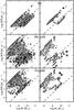 |
Fig. 28 Same as Fig. 20 for three models (top: REF, centre: DEC+NEB, bottom: RIS+NEB) at z ~ 3 (left) and z ~ 6 (right). For z ~ 6, models with declining and rising SF include Lyα. |
For declining SF or other episodic star formation histories, it becomes very difficult to connect galaxy populations at different redshifts and to draw conclusions from such a comparison. This is, of course, due to strong changes in UV luminosity with time and it would lead also to incorrect estimates of some parameters due to the “outshining” effect, where the glare of young massive stars can hide the properties of older stellar population. For example, Papovich et al. (2001) estimates that an hypothetical old stellar population could contain up to ~3–8 times the stellar mass of the young stars that dominate the observed SED.
However, Stark et al. (2009) predict the presence of massive objects with low star-forming activity under the assumption of an episodic star formation model. Since active and quiescent galaxies have similar distribution in stellar mass from z ~ 5 to z ~ 3 and a significant difference in median SFR (~ 0.6 dex), we can interpret this result as a confirmation of this prediction.
A consequence of episodic SF is that age becomes a poorly constrained parameter. It is also difficult to place constraints on the timescale of activity and inactivity and, indeed, to determine if the estimated parameters at different redshift are consistent with this scenario. Lee et al. (2009a) provide a higher limit on duration of star formation activity of 350 Myr based on observed UV luminosity function and clustering at z ~ 4 and z ~ 5. At high-redshift (z ≳ 6) Wyithe & Loeb (2011) found that the starburst timescale is set by the lifetime of massive stars, by comparing different assumptions on supernova feedback and observed evolution in galaxy size and UV luminosity function. These two results promote short timescales, which seems to be confirmed by our results, while uncertainties remain large. Furthermore, the result of Wyithe & Loeb (2011) implies decreasing timescale with increasing redshift. Figure 28 show the difference in SFR–M⋆ relation between z ~ 3 and z ~ 6. At z ~ 6, active and quiescent galaxies form two clearly separate groups while at z ~ 3, the two groups populate all the intermediate states. We can interpret this result as an evolving star formation timescale, which is shorter at z ~ 6 than at z ~ 3.
Under the assumption of episodic star formation, age becomes a tracer of the most recent star formation episode, since the youngest stars dominate the observed fluxes. This parameter does not allow us to determine if observed high redshift LBGs are progenitors of the observed low redshift LBGs. In this scenario, the number of free parameters (including duration of star-formation activity, duration of inactivity, the possibility for LBGs to evolve into a state with no star formation activity) are too large to conclude.
Several studies (Bouché et al. 2010; Wuyts et al. 2011) suggest other SFHs, such as exponentially increasing or delayed star formation. These scenarios have been studied in Schaerer et al. (2013).
 |
Fig. 29 Median specific star formation rate as a function of redshift for four models with a 68% confidence limit based on the whole probability distribution function with comparison of results from different studies (Noeske et al. 2007; Daddi et al. 2007; Stark et al. 2009; Reddy et al. 2012b) and results from studies accounting for nebular emission effect (Stark et al. 2013; Smit et al. 2013). At z ~ 6, we show results with +NEB+Lyα option for declining and rising SFHs. Typical errors are ~ 0.3 dex. The dashed line shows the relation expected from Bouché et al. (2010) for an exponentially increasing star formation at a fixed M⋆ = 109.5 M⊙. The dotted line given by sSFR = 2 Gyr-1 is shown to guide the eye. |
4.5. Specific star formation rate
Since our study gives some elements supporting episodic star formation histories at high redshift, we compare the evolution of sSFR with results from other studies in Fig. 29, using the compilation from González et al. (2010), which is given at fixed stellar mass M⋆ = 5 × 10⁹ M⊙ (Noeske et al. 2007; Daddi et al. 2007; Stark et al. 2009). Since our different models lead to significant different median stellar masses (for e.g., 109.6 M⊙ for REF model at z ~ 3 and 108.6 M⊙ for DEC+NEB+Lyα model at z ~ 6), we compare the median sSFR for entire samples at each redshift. Typically, other studies found no significant change in median stellar mass with redshift and the median value of sSFR at M⋆ = 5 × 10⁹ M⊙ is near the median value for the whole sample (e.g. González et al. 2010). Due to incompleteness, our values can be considered as a lower limit, since we find a trend of increasing sSFR with decreasing stellar mass for all models, albeit this trend is moderate with constant star formation (see Fig. 21). However, we cannot exclude the presence at these redshift of star forming galaxies enshrouded with dust, so our results have to be considered with appropriate caution. The impact of nebular emission on the sSFR evolution with redshift is also considered in Stark et al. (2013) and Smit et al. (2013), and while these studies conclude that the sSFR is higher than in previous studies not accounting for nebular emission, the exact evolutionary trend remains very uncertain. However, these studies confirm our main result: nebular emission can have a significant impact on stellar mass and star formation rate estimation at high-redshift.
Summary of other studies in the literature as compared with our results.
While our results for constant star formation seem to be consistent with those of Stark et al. (2009) for z ~ 4 and z ~ 5, we find a higher median sSFR at z ~ 6. Looking at IRAC channels, galaxies at z ~ 6 with high sSFR (~20 Gyr-1) have on average 2 to 3 channels with no detection (or no data), while galaxies with lower sSFR (median ~1.7 Gyr-1) have typically no more than 1 channel with no detection. No detection in the (rest-frame) optical bands leads to lower stellar mass estimation (~1 dex), while the estimated SFR stays similar. This explains the higher sSFR found for the REF models at z ~ 6 compared to Stark et al. (2009). It is difficult to conclude if it is an effect due only to the lack of IRAC detection, or if it is physical. However, the difference of IRAC detections among the objects should correlate with physical differences in stellar mass. The precise extent of these differences is more difficult to constrain; additional data are needed. The consideration of nebular emission with a constant star formation (REF+NEB) leads to higher sSFRs, and an evolution compatible with the trend from (Bouché et al. 2010). This increase in sSFR is mainly due to a slight decrease in stellar mass estimation with a redshift due to an increase in emission lines strength with redshift (see Table 2).
Our results with declining and rising star formation, which includes nebular emission, differ significantly from previous studies, with a higher median sSFR and a trend of increasing sSFR with redshift. Large confidence limits are due to a large dispersion of individual objects. For DEC+NEB and RIS+NEB, this dispersion is larger due to the two different LBG populations of “weak” and “strong” emitters. While studies neglecting nebular emission lead to the conclusion that star formation seems to be driven by different principles below and above z ~ 2, the different assumptions used here and the results provided by DEC+NEB and RIS+NEB models highlight the possibility to reconcile theoretical expectations with inferred physical parameters.
5. Discussion
5.1. Do we obtain realistic ages?
Since we have not imposed a lower limit for age estimation for both declining and rising SF, both models lead to a significant number of galaxies with an age below a typical dynamical timescale, especially for active galaxies (i.e. “strong” emitters). Indeed, the median ages for this latter population are almost always close to our dynamical time estimate (Sect. 4.3.5). Since the age estimation depends on star formation timescale for declining SF, we test some fixed values of τ to examine the effect on age and other parameters estimation. With τ = 100 Myr, we do not observe any significant change in median values of the different parameters, except for age, which increases by a factor ~ 2.5 for both active and quiescent galaxies (i.e. “weak” galaxies) at each redshift. However, if we look at the age distribution, there is still a significant number of galaxies with age t < tdyn. Imposing a lower limit of ~40 Myr leads to an explanation of the previous result: nebular emission of active galaxies seems to be correctly fit only with very young ages. Using our sample at z ϵ [3.8, 5] with 3.6 μm and 4.5 μm fluxes measured, both declining and rising models are then not any more able to produce a significantly better fit of 3.6 μm–4.5 μm colour (in comparison with the REF model), which is correlated with EW(Hα).
While this discrepancy between a significant fraction of our estimated ages and dynamical
timescale may be a concern for our study, we are reminded of two elements. First,
declining and rising models lead to higher uncertainty on age, which are typically by a
factor ~3 when nebular
emission is considered and can allow us to reconcile almost 80% of our samples with the
dynamical timescale. Second, there is no measured velocity dispersion of nebular lines at
z > 3, since this measurement
is confronted to the limit of current facilities. Furthermore, we use typical velocity
dispersion measurements at z ~ 2 ( km s-1, with a 7 km s-1 error in the mean, Förster Schreiber et al. 2009), which lead to a
~40% possible variation in
the dynamical timescale of individual galaxies for a given typical rhl.
km s-1, with a 7 km s-1 error in the mean, Förster Schreiber et al. 2009), which lead to a
~40% possible variation in
the dynamical timescale of individual galaxies for a given typical rhl.
We conclude that apparent discrepancies between dynamical timescale and estimated ages in this study are considerably reduced when uncertainties on estimated age and typical dispersions on velocity dispersion are taken into account. For rising and declining SFH, the estimated age of a fraction of LBGs (~20%) are inconsistent with dynamical timescale, mainly because of the strength of some lines (e.g. Hα), which can be reproduced by our SED fitting code with this set of assumptions only with extremely young ages.
5.2. Comparison with other studies
During the last decade, various papers presented analyse of LBG properties at high redshift. Since we use a large range of star formation histories, we are able to compare our results to several of them, which are carried out for several LBG samples between z ~ 3 and 6. The main assumptions made for the SED fits in these papers, size of their galaxy samples, and our corresponding models for comparison are listed in Table 3. To allow straightforward comparisons, we use the median/mean values derived from our probability distribution functions. Except stated otherwise, we determine the mean over our entire samples. Although derived from the same pdfs, the values from our models quoted here do therefore not correspond to values listed in Tables A.1–A.3 (which are median values, not mean values).
Shapley et al. (2001, hereafter S01) and Papovich et al. (2001, hereafter P01) have studied 74 and 33 LBGs respectively, at z ~ 3. The S01 sample is restricted to brighter objects (MUV ≲ −20.7) than the sample studied here; thus, we use a subsample of our z ~ 3 LBGs with the same magnitude limit. Note that both studies (S01 and P01) include photometry up to the K-band and not longward. For both studies, we find very similar results for median ages (S01 obtain ~350 Myr and P01 ~70 Myr) and age distributions when corresponding models without nebular emission are used. This is not surprising since age is mainly constrained by the presence of the Balmer Break, which both studies can constrain from KS and J (or H) band data. We also find a similar median stellar mass compared to P01 (3 × 10⁹M⊙), while we obtain mean stellar mass slightly lower by ~0.2 dex compared to S01 (2 × 10¹⁰ M⊙). Since P01 provide best fit parameters for their sample, we can see that significant discrepancies appear on dust attenuation estimation. For both studies extinction factors are ~2 times larger compared to our results. A possible explanation is that we can better constrain this parameter with IRAC data since longer wavelengths are less sensitive to reddening. Furthermore, S01 use a BC96 population synthesis models, while we use BC03 models. Pentericci et al. (2010) have used BC03 models to study a sample of LBGs at z ~ 3, and they found a similar result: same ages and lower dust attenuation in comparison with S01, while they used an exponentially declining SFH. These differences with S01 can come from the use of IRAC data but also from the difference in SFH.
Pentericci et al. (2007, hereafter PG07) and Lee et al. (2011, hereafter L11) provide analysis of 47 and 1913 LBGs at z ~ 4 with indidivual SED fittings in the first case, while L11 uses a stacking procedure in UV magnitude bins. The large sample of L11 has an upper limit MUV = −21.43, at z ~ 3, so we take care to do an appropriate comparison. Our results are similar with those from L11 in stellar mass, age, and dust extinction, although we have only 17 LBGs with MUV ≤ −21.43. A discrepancy appears with the results from PG07, since we find a lower mean stellar mass by ~0.4 dex, while age, dust extinction, and SFRs are similar.
Stellar masses at z ~ 5 and 6 are also in good agreement with previous studies, when the same/similar assumptions are used. Concretely, V07 found a median stellar mass of 2 × 10⁹ M⊙ (3.6 × 10⁹ M⊙ for our study), and Y09 and S07 found a mean stellar mass of 4.1 × 10⁹ and 7.9 × 10⁹ M⊙ respectively at z ~ 5 (while we find 9.9 × 10⁹ and 1.2 × 10¹⁰M⊙ with REF and DEC models respectively). At z ~ 6, Y06 and E07 found 9.6 × 10⁹ and 1.6 × 10¹⁰ M⊙ respectively, as compared to our masses of 9.9 × 10⁹ and 1.1 × 10¹⁰M⊙. The consistency of our results with other studies, by considering typical uncertainty of ~0.15 dex for REF model and ~0.2 dex for DEC model, confirm that stellar mass is the most reliable parameter, since different assumptions on star formation history and also extinction law lead to similar results (cf. Papovich et al. 2001; Verma et al. 2007; Yabe et al. 2009).
Ages of z ~ 5–6 LBGs obtained in the literature agree overall with our results, except for the study of Verma et al. (2007). Compared to their young median age of 25 Myr, we find 255 Myr, a difference which cannot be explained by uncertainty (~0.15 dex for REF model and ~0.4 dex for DEC model). A possible explanation for the discrepancy with V07 could be the age-reddening degeneracy. However, V07 found a median AV = 0.3 mag, while we find 0.2 mag, which cannot explain the difference on the median age estimate. The origin of this difference remains unclear. On the other hand, Y09 and S07 found median ages of 25 Myr and 288 Myr (compared to 52 Myr and 320 Myr from our study) at z ~ 5, and Y06 and E07 obtained 290 Myr and 400 Myr (262 Myr and 190 Myr) at z ~ 6, which are values in good agreement with our results.
Other differences appear on the reddening estimates: while Y09 found a mean AV ~ 0.9 mag at z ~ 5, we obtain 0.4 mag for the corresponding constant SFR model (typical uncertainty ~0.1 mag). At z ~ 6, E07 found no reddening on average, while we obtain AV = 0.4 for the DEC model (typical uncertainty ~ 0.25 mag). Our result at z ~ 5 with the DEC model (mean AV = 0.4) is consistent with S07, since they found the same mean reddening. The differences on dust reddening estimation can have several explanations: the limited size of the samples compared to ours, or the lack of deep near-IR and IRAC photometry which are able to put stronger constraints both on reddening and age. However, these latter arguments cannot be used to explain the discrepancy with Y09, and we do not find a satisfactory explanation.
These discrepancies on reddening must obviously lead to differences on the derived star formation rates. Indeed, Y09 found a mean SFR of 141 M⊙ yr-1 and V07 found a median SFR of 40 M⊙ yr-1 at z ~ 5, while we find ~ 50 M⊙ yr-1 and 15 M⊙ yr-1 from the models that best correspond to their assumptions. The difference on reddening estimation with Y09 explains the difference on SFR estimation, while the result of V07 can be explained by their very young median age, which leads to a significant deviation from the Kennicutt relation (Kennicutt 1998), and thus to a higher SFR. The sample from S07 does not provide SFR estimations but Y09 fits the parameters of S07: a median value of 20 M⊙ yr-1 was found, which is consistent with our result. However, these refitted parameters differ significantly from the results of S07 for both stellar mass and age, which casts some doubt on the homogeneity of this comparison. For z ~ 6, Y06 and E07 found a mean SFR ≲ 10 M⊙ yr-1. While our results are consistent with Y06 (7 M⊙ yr-1), our SFR estimation differs significantly from E07 with an higher SFR (~ 80 M⊙ yr-1). This latter difference can be explained by the higher estimated dust reddening, since E07 estimates that z ~ 6 galaxies are mainly dust free.
Overall, we find good agreement with other studies in general for identical assumptions. Exceptions are the young ages of V07 and high dust extinction of Y09. When nebular emission is included, however the results change significantly, as we have shown in this study.
5.2.1. Evolution of the mass–UV magnitude relation?
Stark et al. (2009) and González et al. (2011) cover a range of redshift between z ~ 4 to z ~ 6 (up to z ~ 7 for the latter). Both studies present the M⋆–MUV relation, which can be directly compared with our results in Figs. 14 and 27. As already discussed in Sect. 4.3.6, we find similar results as González et al. (2011), although our models for exponentially declining and for the rising star formation history suggest lower masses at high UV luminosities. Overall our relations remain within the scatter of ± 0.5 indicated by their work.
Both Stark et al. (2009) and González et al. (2011) find no evolution of the mass – UV magnitude relation with redshift. In contrast, our results seem to indicate a change of the M⋆–MUV relation between z ~ 5 and 6, as shown in Fig. 30. (cf. also Sect. 4.4.4). The main reason for this change is due to our finding of relatively young ages for z ~ 6 galaxies, which implies a lower M/LUV ratio. This effect was also noticed by McLure et al. (2011) for their z ~ 6–8 sample. A reanalysis of their sample with the same method and assumptions used in the present paper confirms our finding from the z ~ 6 sample (Schaerer & de Barros, in prep.).
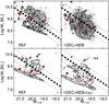 |
Fig. 30 Composite probability distribution of M1500 and M⋆ for REF and DEC+NEB(+Lyα) models at z ~ 5 and z ~ 6. The dashed black line represents the M⋆–M1500 trend found by González et al. (2011) and dotted black lines show a scatter of ±0.5 dex. The points overlaid show the median value properties for each object in the sample: black dots for “weak” nebular emitters, and white dots for “strong” nebular emitters. The overlaid contour indicates the 68% integrated probabilities on the ensemble properties measured from the centroid of the distribution. Red dots are median values of M⋆ in MUV bins. |
5.2.2. LBGs with strong emission lines
An important finding from our quantitative models of LBGs with spectral models that include nebular lines is the distinction of two separate categories of galaxies identified as ”strong” and “weak” nebular emitters (cf. Sect. 4.1) Our work has revealed these categories from comparisons of the fit quality for models with and without nebular emission, and interestingly we found approximately the same fraction of objects (~2/3 strong versus 1/3 weak emitters) at each redshift.
As already mentioned above, two other studies of z ~ 4–5 LBGs have previously found similar objects with strong Hα emission identified by their excess in the 3.6 μm filter with respect to 4.5 μm. From a sample of 74 LBGs with spectroscopic redshifts between 3.8 and 5, Shim et al. (2011) found at least 65% of galaxies that show a 3.6 μm excess attributed to Hα (cf. also Stark et al. 2013, for a recent confirmation). Earlier, Yabe et al. (2009) had already noted a 3.6 μm excess for 70% of their z ~ 5 LBG sample of ~100 galaxies, which attributed to the same effect. Obviously our study finds the same result and a very similar percentage of galaxies. Our work carries this result further by revealing the existence of these two LBG categories among all the samples studied here, ranging from U drops to i drops (i.e. z ~ 3–6), and extending this result to fainter objects, for which no spectroscopy is currently available.
Besides this important agreement, our results differ, however, on severals points from those of Shim et al. (2011). For example, these authors conclude that 60% of their so-called Hα emitters are forming stars at a relatively constant rate by comparing estimated Hα equivalent width (obtained from the 3.6 μm excess) and ages from broadband SED fits, whereas the rest prefer a more “bursty” star formation. Our models yield nearly opposite results (cf. Sect. 4.2). Since the effects of nebular emission affect the estimated ages in particular, the models of Shim et al. (2011), which neglect these effects in their SED modelling, cannot give consistent physical parameters for their strong Hα emitters. Similarly, whereas Shim et al. (2011) prefer the SMC extinction law, our calculations for the B-drop sample using this law show that the vast majority of objects is a better fit with the Calzetti attenuation law, when accounting for nebular emission. Finally, we see no need for a top-heavy IMF or extremely low metallicities from our models, as suggested as possible causes of the strong Hα emission by Shim et al. (2011). In any case, the Hα star formation rates and the Hα equivalent widths derived in Shim et al. (2011) are comparable to ours.
5.3. Remaining uncertainties
5.3.1. Uncertainties affecting individual objects
Our study illustrates the way various physical parameters depend on model assumptions made for the broadband SED fits in detail, and a large range of parameter space has been explored here. Despite these extensive investigations, the impact of some assumptions have not been explored in depth, and several uncertainties remain.
The impact of different extinction laws, for example, has hardly been discussed here. Several papers presenting SED fits of LBGs at different redshifts have examined the differences obtained with the Calzetti attenuation law (adopted here) and the SMC extinction law (Prevot et al. 1984; Bouchet et al. 1985). Among them are the work of Papovich et al. (2001), Verma et al. (2007), and Yabe et al. (2009) who study LBG samples at z ~ 3 and 5. A comprehensive comparison of the impact of different extinction laws (including SMC, LMC, Galactic, and the Calzetti law) is presented in Yabe et al. (2009). To examine how different extinction laws modify the results from SED fitting models that include nebular emission, we have modeled the B-drop sample with the declining star formation history (DEC+NEB model) by adopting the SMC law of (Prevot et al. 1984). Qualitatively, our results show the same trends as found by Yabe et al. (2009); that is, there is no big difference on stellar masses, lower AV, older ages, and lower SFR. However, we find that the Calzetti attenuation law provides a better fit for the vast majority of galaxies. Except for a few special cases such as the lensed galaxies, cB58 and the Cosmic Eye, which are studied in detail and at different wavelengths but also include the IR (see Siana et al. 2008; Wuyts et al. 2011, but cf. Sklias et al. 2014) SMC law appears to be favoured from the measurement of the IR/UV luminosity and the UV slope. It is generally thought that the Calzetti attenuation law is applicable (at least on average) to high redshift star forming galaxies (but see Shim et al. 2011; Oesch et al. 2013).
Our models that include the effects of nebular emission assumed case B recombination to compute the strength of the hydrogen recombination lines (and empirical line ratios for other lines from He and metals) and of nebular continuum emission. In particular we thereby assume that all Lyman continuum photons contribute to nebular emission, which neglects therefore possible losses of ionizing photons due to dust inside HII regions or to escape of Lyman continuum photons. Furthermore, we assume the same extinction/attenuation for stellar and nebular emission, whereas observations of nearby galaxies indicate that emission lines usually suffer from a higher extinction than the stellar continuum (cf. Calzetti et al. 2000). In this sense, our models maximize the effects of nebular emission, whereas the lines could be weaker than predicted by our models in reality. On the other hand, we have adopted empirical line ratios compiled by Anders & Fritze-v. Alvensleben (2003) from nearby galaxies, whereas the conditions in distant galaxies could be different, which leads to higher excitation or stronger lines (Erb et al. 2010; Kewley et al. 2013; Nakajima & Ouchi 2013).
These uncertainties are currently difficult to quantify. In any case, the broadband SEDs clearly reveal the presence of nebular lines, and our models include a wide range between maximum and no nebular emission. Future spectroscopic observations or narrow/intermediate band imaging should try to provide more detailed and accurate observational constraints on the emission line strengths of LBGs at high redshift. Detailed predictions from our models that regard individual lines will be presented elsewhere and can be made available on request.
As clearly shown by our study, assumptions on the star formation history have a significant impact on the estimated physical parameters when broadband SED fits are used. Although certain star formation histories are found to provide better fits than others (cf. Sect. 4.2), it is obvious that the simple parametrisations commonly adopted in literature and in our study can only be very crude representations of the true SF histories of individual galaxies. In a companion paper (Schaerer et al. 2013), we have explored two additional families of star formation histories, a so-called delayed star formation (SFR ∝ texp(−t/τ)) and exponentially rising histories with variable timescales. Using arbitrary star formation histories is, however, not practical, given the limited number of observational constraints. Another approach has been taken by Finlator et al. (2007), who have used the star formation history from their cosmological hydrodynamic simulations to fit observed high-z galaxies. However, such studies have so far been limited to a very small number of galaxies. Future improvements on this issue from both observations and simulations are certainly needed. For example, Reddy et al. (2012b) test different SF histories using IR and UV observations of z ~ 2 LBGs. Along similar lines, we show in Schaerer et al. (2013) how SFHs can be distinguished by measuring their dust emission with future ALMA observations and/or with measurements of emission lines. Sklias et al. (2014) have carried out such an analysis for 7 lensed galaxies using recent Herschel observations.
5.3.2. Biases and selection effects
For obvious reasons, selection effects and various biases affect studies in general of galaxy populations, and these need to be taken into account to compare different samples in the analysis of apparent correlations between derived physical parameters and in other contexts.
To allow meaningful comparisons with other studies, we have presented our detailed results in bins of UV magnitude (see data in Tables A.1–A.3). Especially in the brightest and faintest bins, the number of galaxies is low, so that these results should be taken with care. Of course, the number of galaxies at different redshifts varies strongly, affecting the accuracy of the median physical properties (and confidence range) derived here.
As in most literature studies, selection effects and biases have not been treated here. The impact of biases on the determination of physical parameters of LBGs from broadband SED fitting has been studied by Lee et al. (2009b), who constructs mock galaxy catalogues from semi-analytical models, which are then used to fit the simulated galaxies with a standard SED fitting tool. They find that stellar masses can be recovered well, whereas single-component SED fitting methods underestimate SFRs and overestimate ages. The differences are attributed in part to a “mismatch” of star formation histories between their fitting tool (which assumes exponentially declining SF) and those predicted by their galaxy models (which are often rising). A similar “template mismatch” was also identified as the main cause for differences in the comparison of z ~ 1.5–3 merger simulations with SED fitting results carried out by Wuyts et al. (2009). Our models are also prone to such biases/uncertainties, and the role of the assumed SF histories on the derived physical parameters has already been discussed above. However, since we have covered a wider range of SFHs including rising SF, our results may suffer less from this potential problem. The results from SED fits with additional SFHs (including exponentially declining histories with adjustable timescales) are presented in Schaerer et al. (2013).
Various correlations have been found between physical parameters as the stellar mass, the star formation rate, age, and others in both the literature and in our study. Although our work emphasizes the way the physical parameters depend on various model assumptions, it is important to be aware of the selection effects that may significantly affect such correlations. Stringer et al. (2011) have recently examined the behaviour of the SFR and the specific SFR with stellar mass, two important quantities discussed extensively in the recent literature. From their simulations of mock galaxies to which observational selection criteria and “standard” analysis are applied, they show how true underlying trends can be misrepresented. This study also echoes the caution expressed by Dunne et al. (2009) on the apparent sSFR–mass relation, which they urge, could be severely affected by selection biases. Reddy et al. (2012b) also discussed how the Malmquist bias in UV-selected sample can affect the SFR–M⋆ relation, and thus the sSFR determination. To the best of our knowledge, the effect and extent of selection effects and biases on apparent correlation between extinction and mass, and age and mass (cf. Sect. 4.3.6) has not yet been addressed. A quantitative study of these effects is clearly beyond the scope of the present publication.
6. Summary and conclusions
We present a homogeneous study of a sample of ~ 1700 LBGs at z ~ 3−6 from the GOODS-MUSIC catalogue (Santini et al. 2009) with deep photometry from the U band to 8 μm. Using a modified version of the HyperZ photometric redshift code that takes into account nebular emission (Schaerer & de Barros 2009), we explore a range of star formation history (constant, exponentially decreasing, and rising). We explore a wide parameter space in redshift, metallicity, age, and extinction as described by the Calzetti law (Calzetti et al. 2000) by varying e-folding timescales for star formation and determining whether or not nebular emission is included. The main physical parameters derived from our models are the stellar mass, age, reddening, star formation rate SFR, and specific SFR. Furthermore, our models also provide information on the characteristic SF timescale.
Our method and the selected sample has been described in Sects. 2 and 3. The detailed model results concerning the physical parameters, correlations among them, and the redshift evolution of the galaxy properties have been presented in Sect. 4. Our main results can be summarized as follows:
-
Independent of the adopted star formation history, we find that ~65% of the galaxies are better fit with nebular emission and ~35% without (Fig. 3) at all redshifts. According to the Akaike Information Criterium, models that include nebular emission are 5−10 times more likely to be better model than models without nebular emission for the first group (i.e ~65% of the galaxies), while the rest shows a probability two times larger to be best fit by models without nebular emission. For galaxies with zϵ [3.8, 5], these two groups are clearly identified by their 3.6 μm−4.5 μm colour (Fig. 4), which is correlated with strong Hα emission (cf. Shim et al. 2011). Furthermore, this colour cannot be reproduced if we impose an age limitation >50 Myr (Fig. 5). This observed colour distribution clearly indicates the existence of galaxies with strong emission lines and others with few or no discernible signs of emission lines (see Table 2). Our SED modelling reveals the presence of two LBG groups (dubbed “strong” and “weak” emitters respectively) at all redshifts studied here (z ~ 3–6) from U drops to i drops.
-
Models that include the effects of nebular emission and account for variable (declining or rising) star formation histories naturally separate the two LBG groups according to current star formation rate, where the group of “strong” emitters show a larger SFR than the “weak” emitters (Fig. 20). In a scenario of declining star formation histories, these groups could be seen as starbursts and “post-starbursts” with age differences compatible with this suggestion. Indeed, properties of “weak” emitters are compatible with slightly more evolved population with older ages, lower dust attenuation, and slightly lower stellar mass and SFR, when compared to “strong” emitters. Models with constant SFR, nebular emission, and age >50 Myr cannot reproduce the observed range of 3.6μm−4.5μm colours of z ~ 3.8–5 galaxies.
-
Independent of the star formation history, the inclusion of nebular emission leads to younger ages on average (Fig. 6), since nebular lines in optical (rest-frame) are able to mimic a Balmer break. This confirms our earlier findings (Schaerer & de Barros 2009, 2010) for larger samples and over a wider redshift range.
-
We find that the derived dust attenuation mainly depends on the assumed star formation history and that the treatment of nebular emission does not lead to a general systematic shift. Discrepancies found between our results with decreasing SFH and those from other studies at z ~ 2 (e.g. Shapley et al. 2005; Erb et al. 2006b; Reddy et al. 2012b) seem to come from modelling assumptions on both age and metallicity. The largest attenuation is found with rising star formation histories, since these always predict very recent star formation and hence UV emission, as already discussed by Schaerer & Pelló (2005). In this case, the inclusion of nebular emission decreases the average attenuation, whereas the attenuation increases for declining SFHs, and remains unchanged for constant SFR.
-
Based on our SED fits of 700 z ~ 4 LBGs, we propose a new average relation between the observed UV slope β and the attenuation AV. Our relation deviates from the classical relation (Meurer et al. 1999), which assumes constant SFR, ages ≳100 Myr and solar metallicity, and leads to a higher attenuation for a given β slope.
-
Considering nebular emission, the stellar masses derived from the SED fits decrease by ~0.4 on average and by larger amounts (~0.4−0.9 dex) for LBGs from the “strong” emitter group (Fig. 13). We find a trend of increasing dust attenuation with stellar mass (Fig. 16), as already suggested earlier for z ~ 6–8 galaxies (Schaerer & de Barros 2010), and a trend of increasing age with galaxy mass (Fig. 15).
-
Given the large scatter found in the SFR–M⋆ relation for all models with variable star formation histories, we also find a large scatter for the specific star formation rate sSFR with stellar mass and at all redshifts. Our favoured models show a higher median sSFR at z ~ 3−6 than derived by previous studies (e.g. González et al. 2011). Our results tend to indicate an increase of the median sSFR with redshift, as advocated by several theoretical galaxy formation and evolution models (Bouché et al. 2010; Dutton et al. 2010; Weinmann et al. 2011).
-
While uncertainties on τ remain large, our SED fits favour short median star formation timescales (≲300 Myr). Furthermore, we find tentative evidence of decreasing values of τ with decreasing UV luminosity among the sample of “strong” emitters.
-
As already shown in Stark et al. (2009), constant star formation seems to be irreconcilable with the non-evolution of the M⋆ − M1500 relation between z ~ 5 to 3 and with the UV luminosity function.
-
The rising average star formation of Finlator et al. (2011) used in this study cannot represent the typical history of many individual LBGs over long time, since the predicted increase if continuing into the future, is too fast. This would lead to a strong increase of median stellar masses and the median SFR from one redshift to another, which would also imply an increase in dust attenuation to hide these objects from the LBG selection, since this very massive and strongly star-forming galaxies are not seen in the expected numbers (cf. Reddy et al. 2012b).
-
Two groups of LBGs identified as active and more quiescent galaxies (respectively “strong” and “weak” emitters, Fig. 20) are present. Our finding of best SED fits with declining star formation histories and the consistency of these results with constraints on duty cycles from clustering studies and other theoretical arguments (Lee et al. 2009a; Wyithe & Loeb 2011) all concur to consider episodic star formation as the scenario that best fits observations of LBGs at high redshift.
Our systematic and homogeneous analysis casts new light on the physical properties of LBGs from z ~ 3 to 6 and possibly to higher redshift (cf. Schaerer & de Barros 2010). Obviously, our results have a potentially important impact on a variety of questions, and several implications need to be worked out. On the other hand, our study also calls for new observations and tests.
For example, both our preferred models (variable star formation histories with nebular emission) imply a higher UV attenuation than what is currently derived, using the observed UV slope. At z ~ 4, our models typically predict an increase by a factor ≲3 but smaller changes at higher redshift. Implications on the cosmic star formation history and related topics will be worked out in a separate publication. If correct, a higher UV attenuation should lead to measurable changes in the IR emission of LBGs. A stacking analysis of the LBGs studied in this paper shows that the models presented here are all compatible with the current IR, sub-mm, and radio observations (Greve et al., in prep.). Detailed predictions of the IR-mm emission from our galaxies are presented in Schaerer et al. (2013). More sensitive observations in the future with ALMA should be able to detect individual LBGs over a wide redshift range, to determine their attenuation, and, hence, to also distinguish different star formation histories (Shim et al. 2011; Schaerer et al. 2013).
An important implication from our study is that the idea of a simple, well-defined “star formation main sequence” with the majority of star forming galaxies that show tight relation between SFR and M⋆, as suggested from other studies at lower redshift (z ~ 0–2, cf. Daddi et al. 2007; Elbaz et al. 2007; Noeske et al. 2007), may not be appropriate at high redshift (z ≳ 3). Indeed, a relatively small scatter is only obtained assuming constant star formation over long enough timescales (≳50 Myr), whereas our models clearly provide indications for variable star formation histories and episodic star formation (cf. Sects. 4.3.5, 4.2). A significant scatter is also obtained for models assuming rising or delayed star formation histories (see Sect. 4.3.7 and Schaerer et al. 2013), which are often suggested in the literature. If the scatter found from our models in the SFR–M⋆ relation decreases with decreasing redshift, convergence towards the results from other studies remains to be seen. However, a smaller scatter is naturally found since constant star formation is usually assumed in most models for establishing the standard SFR calibrations used in the literature (Daddi et al. 2007; Elbaz et al. 2007; González et al. 2011; Wuyts et al. 2011) or when analyzing stacked data, which naturally smoothes out any possible variation (Lee et al. 2010). Establishing more precisely the attenuation, current SFR and star formation histories of galaxies is therefore crucial to shed more light on these questions.
Related to the above mentioned scatter is also the behaviour of the specific star formation rate (sSFR) with both galaxy mass and on average with redshift. Basically, the same questions and uncertainties concerning the SFR–M⋆ relation apply here. In any case, it must be recognized that the sSFR is strongly dependent on model assumptions and seems to show a strong dependence on the galaxy mass. Whereas earlier determinations of the sSFR at z > 3 were considered in conflict with recent galaxy evolution models (Bouché et al. 2010), our results are clearly in better agreement with the high sSFR values and the redshift evolution predicted by these models. A detailed confrontation of our results with such models and more refined ones will hopefully provide further insight into galaxy formation and evolution models at high redshift.
Finally, it is clear that our study reveals new aspects on the possibly complex and variable star formation histories of high redshift galaxies. Whereas different arguments are found in the literature that favour short duty cycles and episodic star formation (cf. Sawicki & Yee 1998; Verma et al. 2007; Stark et al. 2009; Lee et al. 2009a; Wyithe & Loeb 2011) based on SED studies, LBG clustering, and other arguments, other studies favour long star formation timescales (Shapley et al. 2001; Lee et al. 2011; Shim et al. 2011). Our study uses quantitatively features probing emission lines for the first time, whose strength is naturally sensitive to relatively rapid variations in the recent SFR. Although such variations have been more difficult to uncover before, this may therefore not be surprising. Direct observations of the emission lines in high-z LBGs should be very useful to test our models and provide more stringent constraints on the importance of nebular emission and on the star formation histories of distant galaxies (Schaerer et al. 2013). Other studies providing new measurement of LBG clustering at z > 4, searches for passive galaxies at high redshift, or theoretical studies on star formation and regulation processes can also help to improve our understanding of these important issues closely related to key questions on galaxy formation and evolution.
Online material
Appendix A
Galaxy properties over 3 ≤ z ≤ 6 for constant star formation and solar metallicity set of models in M1500 bins.
Rising SFHs with varying timescales have been explored in Schaerer et al. (2013).
It must be recognized that the average SFH derived by Papovich et al. (2011) corresponds to a cosmologically averaged history, which a priori does not apply to individual galaxies.
Acknowledgments
We would like to thank numerous colleagues who have contributed to interesting discussions and raised useful questions during the time when this work was being carried out. We thank them here collectively. We acknowledge the GOODS-MUSIC collaboration. We thank the referee for useful comments and suggestions that helped to improve the quality and presentation of this paper. The work of S.d.B. and D.S. is supported by the Swiss National Science Foundation. D.P.S. is supported by an STFC postdoctoral research fellowship. S.d.B. wants to dedicate this work to the memory of Jean Faure-Brac.
References
- Acquaviva, V., Vargas, C., Gawiser, E., & Guaita, L. 2012, ApJ, 751, L26 [NASA ADS] [CrossRef] [Google Scholar]
- Anders, P., & Fritze-v. Alvensleben, U. 2003, A&A, 401, 1063 [NASA ADS] [CrossRef] [EDP Sciences] [Google Scholar]
- Ando, M., Ohta, K., Iwata, I., et al. 2006, ApJ, 645, L9 [NASA ADS] [CrossRef] [Google Scholar]
- Atek, H., Siana, B., Scarlata, C., et al. 2011, ApJ, 743, 121 [NASA ADS] [CrossRef] [Google Scholar]
- Atek, H., Kunth, D., Schaerer, D., et al. 2014, A&A, 561, A89 [NASA ADS] [CrossRef] [EDP Sciences] [Google Scholar]
- Beckwith, S. V. W., Stiavelli, M., Koekemoer, A. M., et al. 2006, AJ, 132, 1729 [NASA ADS] [CrossRef] [Google Scholar]
- Blanc, G. A., Adams, J. J., Gebhardt, K., et al. 2011, ApJ, 736, 31 [NASA ADS] [CrossRef] [Google Scholar]
- Bolzonella, M., Miralles, J., & Pelló, R. 2000, A&A, 363, 476 [NASA ADS] [Google Scholar]
- Bouché, N., Dekel, A., Genzel, R., et al. 2010, ApJ, 718, 1001 [NASA ADS] [CrossRef] [Google Scholar]
- Bouchet, P., Lequeux, J., Maurice, E., Prevot, L., & Prevot-Burnichon, M. L. 1985, A&A, 149, 330 [NASA ADS] [Google Scholar]
- Bouwens, R. J., Illingworth, G. D., Blakeslee, J. P., Broadhurst, T. J., & Franx, M. 2004, ApJ, 611, L1 [NASA ADS] [CrossRef] [Google Scholar]
- Bouwens, R. J., Illingworth, G. D., Franx, M., & Ford, H. 2007, ApJ, 670, 928 [NASA ADS] [CrossRef] [Google Scholar]
- Bouwens, R. J., Illingworth, G. D., Franx, M., et al. 2009, ApJ, 705, 936 [NASA ADS] [CrossRef] [Google Scholar]
- Bouwens, R. J., Illingworth, G. D., Oesch, P. A., et al. 2012, ApJ, 754, 83 [NASA ADS] [CrossRef] [Google Scholar]
- Bouwens, R. J., Illingworth, G. D., Oesch, P. A., et al. 2013, ApJ, submitted [arXiv:1306.2950] [Google Scholar]
- Brinchmann, J., Charlot, S., White, S. D. M., et al. 2004, MNRAS, 351, 1151 [NASA ADS] [CrossRef] [Google Scholar]
- Bruzual, G., & Charlot, S. 2003, MNRAS, 344, 1000 [NASA ADS] [CrossRef] [Google Scholar]
- Buat, V., Iglesias-Páramo, J., Seibert, M., et al. 2005, ApJ, 619, L51 [NASA ADS] [CrossRef] [Google Scholar]
- Buat, V., Boissier, S., Burgarella, D., et al. 2008, A&A, 483, 107 [NASA ADS] [CrossRef] [EDP Sciences] [Google Scholar]
- Bunker, A. J., Stanway, E. R., Ellis, R. S., & McMahon, R. G. 2004, MNRAS, 355, 374 [NASA ADS] [CrossRef] [Google Scholar]
- Burgarella, D., Le Floc’h, E., Takeuchi, T. T., et al. 2007, MNRAS, 380, 986 [NASA ADS] [CrossRef] [Google Scholar]
- Calzetti, D., Armus, L., Bohlin, R. C., et al. 2000, ApJ, 533, 682 [NASA ADS] [CrossRef] [Google Scholar]
- Castellano, M., Fontana, A., Grazian, A., et al. 2012, A&A, 540, A39 [NASA ADS] [CrossRef] [EDP Sciences] [Google Scholar]
- Charlot, S., & Longhetti, M. 2001, MNRAS, 323, 887 [NASA ADS] [CrossRef] [Google Scholar]
- Cristiani, S., Appenzeller, I., Arnouts, S., et al. 2000, A&A, 359, 489 [NASA ADS] [Google Scholar]
- Curtis-Lake, E., McLure, R. J., Pearce, H. J., et al. 2012, MNRAS, 422, 1425 [NASA ADS] [CrossRef] [EDP Sciences] [Google Scholar]
- Daddi, E., Renzini, A., Pirzkal, N., et al. 2005, ApJ, 626, 680 [NASA ADS] [CrossRef] [Google Scholar]
- Daddi, E., Dickinson, M., Morrison, G., et al. 2007, ApJ, 670, 156 [NASA ADS] [CrossRef] [Google Scholar]
- de Barros, S., Schaerer, D., & Stark, D. P. 2011, in SF2A-2011: Proceedings of the Annual meeting of the French Society of Astronomy and Astrophysics, eds. G. Alecian, K. Belkacem, R. Samadi, & D. Valls-Gabaud, 95 [Google Scholar]
- Doherty, M., Bunker, A. J., Ellis, R. S., & McCarthy, P. J. 2005, MNRAS, 361, 525 [NASA ADS] [CrossRef] [Google Scholar]
- Domínguez, A., Siana, B., Henry, A. L., et al. 2013, ApJ, 763, 145 [NASA ADS] [CrossRef] [Google Scholar]
- Douglas, L. S., Bremer, M. N., Lehnert, M. D., Stanway, E. R., & Milvang-Jensen, B. 2010, MNRAS, 409, 1155 [NASA ADS] [CrossRef] [Google Scholar]
- Dunlop, J. S., Rogers, A. B., McLure, R. J., et al. 2013, MNRAS, 432, 3520 [NASA ADS] [CrossRef] [Google Scholar]
- Dunne, L., Ivison, R. J., Maddox, S., et al. 2009, MNRAS, 394, 3 [NASA ADS] [CrossRef] [Google Scholar]
- Dutton, A. A., van den Bosch, F. C., & Dekel, A. 2010, MNRAS, 405, 1690 [NASA ADS] [Google Scholar]
- Elbaz, D., Daddi, E., Le Borgne, D., et al. 2007, A&A, 468, 33 [NASA ADS] [CrossRef] [EDP Sciences] [Google Scholar]
- Erb, D. K., Shapley, A. E., Pettini, M., et al. 2006a, ApJ, 644, 813 [NASA ADS] [CrossRef] [Google Scholar]
- Erb, D. K., Steidel, C. C., Shapley, A. E., et al. 2006b, ApJ, 647, 128 [NASA ADS] [CrossRef] [Google Scholar]
- Erb, D. K., Steidel, C. C., Shapley, A. E., et al. 2006c, ApJ, 646, 107 [NASA ADS] [CrossRef] [Google Scholar]
- Erb, D. K., Pettini, M., Shapley, A. E., et al. 2010, ApJ, 719, 1168 [NASA ADS] [CrossRef] [Google Scholar]
- Eyles, L. P., Bunker, A. J., Stanway, E. R., et al. 2005, MNRAS, 364, 443 [NASA ADS] [CrossRef] [Google Scholar]
- Eyles, L. P., Bunker, A. J., Ellis, R. S., et al. 2007, MNRAS, 374, 910 [NASA ADS] [CrossRef] [Google Scholar]
- Ferguson, H. C., Dickinson, M., Giavalisco, M., et al. 2004, ApJ, 600, L107 [NASA ADS] [CrossRef] [Google Scholar]
- Finkelstein, S. L., Rhoads, J. E., Malhotra, S., Grogin, N., & Wang, J. 2008, ApJ, 678, 655 [NASA ADS] [CrossRef] [Google Scholar]
- Finkelstein, S. L., Papovich, C., Salmon, B., et al. 2012, ApJ, 756, 164 [NASA ADS] [CrossRef] [Google Scholar]
- Finlator, K., Davé, R., & Oppenheimer, B. D. 2007, MNRAS, 376, 1861 [NASA ADS] [CrossRef] [Google Scholar]
- Finlator, K., Oppenheimer, B. D., & Davé, R. 2011, MNRAS, 410, 1703 [NASA ADS] [Google Scholar]
- Fioc, M., & Rocca-Volmerange, B. 1997, A&A, 326, 950 [NASA ADS] [Google Scholar]
- Förster Schreiber, N. M., Genzel, R., Bouché, N., et al. 2009, ApJ, 706, 1364 [NASA ADS] [CrossRef] [Google Scholar]
- Giacconi, R., Zirm, A., Wang, J., et al. 2002, ApJS, 139, 369 [NASA ADS] [CrossRef] [Google Scholar]
- Giavalisco, M., Dickinson, M., Ferguson, H. C., et al. 2004, ApJ, 600, L103 [NASA ADS] [CrossRef] [Google Scholar]
- González, V., Labbé, I., Bouwens, R. J., et al. 2010, ApJ, 713, 115 [NASA ADS] [CrossRef] [Google Scholar]
- González, V., Labbé, I., Bouwens, R. J., et al. 2011, ApJ, 735, L34 [NASA ADS] [CrossRef] [Google Scholar]
- González, V., Bouwens, R., llingworth, G., et al. 2012 [arXiv:1208.4362] [Google Scholar]
- Gronwall, C., Ciardullo, R., Hickey, T., et al. 2007, ApJ, 667, 79 [NASA ADS] [CrossRef] [Google Scholar]
- Hathi, N. P., Malhotra, S., & Rhoads, J. E. 2008, ApJ, 673, 686 [NASA ADS] [CrossRef] [Google Scholar]
- Hayes, M., Schaerer, D., Östlin, G., et al. 2011, ApJ, 730, 8 [NASA ADS] [CrossRef] [Google Scholar]
- Hildebrandt, H., Arnouts, S., Capak, P., et al. 2010, A&A, 523, A31 [NASA ADS] [CrossRef] [EDP Sciences] [Google Scholar]
- Kennicutt, Jr., R. C. 1998, ARA&A, 36, 189 [Google Scholar]
- Kewley, L. J., Maier, C., Yabe, K., et al. 2013, ApJ, 774, L10 [Google Scholar]
- Labbé, I., Oesch, P. A., Bouwens, R. J., et al. 2013, ApJ, 777, L19 [NASA ADS] [CrossRef] [Google Scholar]
- Le Fèvre, O., Saisse, M., Mancini, D., et al. 2003, in Proc. SPIE 4841, eds. M. Iye, & A. F. M. Moorwood, 1670 [Google Scholar]
- Le Fèvre, O., Vettolani, G., Paltani, S., et al. 2004, A&A, 428, 1043 [NASA ADS] [CrossRef] [EDP Sciences] [Google Scholar]
- Lee, K.-S., Giavalisco, M., Conroy, C., et al. 2009a, ApJ, 695, 368 [NASA ADS] [CrossRef] [Google Scholar]
- Lee, S.-K., Idzi, R., Ferguson, H. C., et al. 2009b, ApJS, 184, 100 [NASA ADS] [CrossRef] [Google Scholar]
- Lee, S.-K., Ferguson, H. C., Somerville, R. S., Wiklind, T., & Giavalisco, M. 2010, ApJ, 725, 1644 [NASA ADS] [CrossRef] [EDP Sciences] [Google Scholar]
- Lee, K.-S., Dey, A., Reddy, N., et al. 2011, ApJ, 733, 99 [NASA ADS] [CrossRef] [Google Scholar]
- Leitherer, C., & Heckman, T. M. 1995, ApJS, 96, 9 [NASA ADS] [CrossRef] [Google Scholar]
- Lidman, C., Hayes, M., Jones, D. H., et al. 2012, MNRAS, 420, 1946 [NASA ADS] [CrossRef] [Google Scholar]
- Madau, P. 1995, ApJ, 441, 18 [NASA ADS] [CrossRef] [Google Scholar]
- Madau, P., Pozzetti, L., & Dickinson, M. 1998, ApJ, 498, 106 [NASA ADS] [CrossRef] [Google Scholar]
- Maiolino, R., Nagao, T., Grazian, A., et al. 2008, A&A, 488, 463 [NASA ADS] [CrossRef] [EDP Sciences] [Google Scholar]
- McLinden, E. M., Finkelstein, S. L., Rhoads, J. E., et al. 2011, ApJ, 730, 136 [NASA ADS] [CrossRef] [Google Scholar]
- McLure, R. J., Dunlop, J. S., de Ravel, L., et al. 2011, MNRAS, 418, 2074 [NASA ADS] [CrossRef] [Google Scholar]
- Meurer, G. R., Heckman, T. M., & Calzetti, D. 1999, ApJ, 521, 64 [NASA ADS] [CrossRef] [Google Scholar]
- Mignoli, M., Cimatti, A., Zamorani, G., et al. 2005, A&A, 437, 883 [NASA ADS] [CrossRef] [EDP Sciences] [Google Scholar]
- Nakajima, K., & Ouchi, M. 2013, MNRAS, submitted [arXiv:1309.0207] [Google Scholar]
- Nilsson, K. K., Møller, P., Möller, O., et al. 2007, A&A, 471, 71 [NASA ADS] [CrossRef] [EDP Sciences] [Google Scholar]
- Noeske, K. G., Weiner, B. J., Faber, S. M., et al. 2007, ApJ, 660, L43 [Google Scholar]
- Nonino, M., Dickinson, M., Rosati, P., et al. 2009, ApJS, 183, 244 [NASA ADS] [CrossRef] [Google Scholar]
- Oesch, P. A., Bouwens, R. J., Illingworth, G. D., et al. 2013, ApJ, 773, 75 [NASA ADS] [CrossRef] [Google Scholar]
- Oke, J. B., & Gunn, J. E. 1983, ApJ, 266, 713 [NASA ADS] [CrossRef] [Google Scholar]
- Ono, Y., Ouchi, M., Shimasaku, K., et al. 2010, ApJ, 724, 1524 [NASA ADS] [CrossRef] [Google Scholar]
- Ouchi, M., Shimasaku, K., Akiyama, M., et al. 2008, ApJS, 176, 301 [NASA ADS] [CrossRef] [Google Scholar]
- Papovich, C., Dickinson, M., & Ferguson, H. C. 2001, ApJ, 559, 620 [NASA ADS] [CrossRef] [Google Scholar]
- Papovich, C., Finkelstein, S. L., Ferguson, H. C., Lotz, J. M., & Giavalisco, M. 2011, MNRAS, 412, 1123 [NASA ADS] [Google Scholar]
- Pentericci, L., Grazian, A., Fontana, A., et al. 2007, A&A, 471, 433 [NASA ADS] [CrossRef] [EDP Sciences] [Google Scholar]
- Pentericci, L., Grazian, A., Scarlata, C., et al. 2010, A&A, 514, A64 [NASA ADS] [CrossRef] [EDP Sciences] [Google Scholar]
- Popesso, P., Dickinson, M., Nonino, M., et al. 2009, A&A, 494, 443 [NASA ADS] [CrossRef] [EDP Sciences] [Google Scholar]
- Prevot, M. L., Lequeux, J., Prevot, L., Maurice, E., & Rocca-Volmerange, B. 1984, A&A, 132, 389 [NASA ADS] [Google Scholar]
- Ravikumar, C. D., Puech, M., Flores, H., et al. 2007, A&A, 465, 1099 [NASA ADS] [CrossRef] [EDP Sciences] [Google Scholar]
- Reddy, N. A., & Steidel, C. C. 2004, ApJ, 603, L13 [NASA ADS] [CrossRef] [Google Scholar]
- Reddy, N. A., Steidel, C. C., Fadda, D., et al. 2006, ApJ, 644, 792 [NASA ADS] [CrossRef] [Google Scholar]
- Reddy, N. A., Steidel, C. C., Pettini, M., et al. 2008, ApJS, 175, 48 [NASA ADS] [CrossRef] [Google Scholar]
- Reddy, N. A., Erb, D. K., Pettini, M., Steidel, C. C., & Shapley, A. E. 2010, ApJ, 712, 1070 [NASA ADS] [CrossRef] [Google Scholar]
- Reddy, N., Dickinson, M., Elbaz, D., et al. 2012a, ApJ, 744, 154 [NASA ADS] [CrossRef] [Google Scholar]
- Reddy, N. A., Pettini, M., Steidel, C. C., et al. 2012b, ApJ, 754, 25 [NASA ADS] [CrossRef] [Google Scholar]
- Roche, N. D., Dunlop, J., Caputi, K. I., et al. 2006, MNRAS, 370, 74 [NASA ADS] [Google Scholar]
- Salpeter, E. E. 1955, ApJ, 121, 161 [Google Scholar]
- Santini, P., Fontana, A., Grazian, A., et al. 2009, A&A, 504, 751 [NASA ADS] [CrossRef] [EDP Sciences] [Google Scholar]
- Sawicki, M. 2012, MNRAS, 421, 2187 [NASA ADS] [CrossRef] [Google Scholar]
- Sawicki, M., & Yee, H. K. C. 1998, AJ, 115, 1329 [NASA ADS] [CrossRef] [Google Scholar]
- Schaerer, D., & de Barros, S. 2009, A&A, 502, 423 [NASA ADS] [CrossRef] [EDP Sciences] [Google Scholar]
- Schaerer, D., & de Barros, S. 2010, A&A, 515, A73 [NASA ADS] [CrossRef] [EDP Sciences] [Google Scholar]
- Schaerer, D., & de Barros, S. 2012, IAU Symp., 284, 20 [NASA ADS] [Google Scholar]
- Schaerer, D., & Pelló, R. 2005, MNRAS, 362, 1054 [NASA ADS] [CrossRef] [Google Scholar]
- Schaerer, D., de Barros, S., & Stark, D. P. 2011, A&A, 536, A72 [NASA ADS] [CrossRef] [EDP Sciences] [Google Scholar]
- Schaerer, D., de Barros, S., & Sklias, P. 2013, A&A, 549, A4 [NASA ADS] [CrossRef] [EDP Sciences] [Google Scholar]
- Schenker, M. A., Stark, D. P., Ellis, R. S., et al. 2012, ApJ, 744, 179 [NASA ADS] [CrossRef] [Google Scholar]
- Schenker, M. A., Ellis, R. S., Konidaris, N. P., & Stark, D. P. 2013, ApJ, 777, 67 [NASA ADS] [CrossRef] [Google Scholar]
- Shapley, A. E., Steidel, C. C., Adelberger, K. L., et al. 2001, ApJ, 562, 95 [NASA ADS] [CrossRef] [Google Scholar]
- Shapley, A. E., Steidel, C. C., Pettini, M., & Adelberger, K. L. 2003, ApJ, 588, 65 [NASA ADS] [CrossRef] [Google Scholar]
- Shapley, A. E., Steidel, C. C., Erb, D. K., et al. 2005, ApJ, 626, 698 [NASA ADS] [CrossRef] [Google Scholar]
- Shim, H., Chary, R.-R., Dickinson, M., et al. 2011, ApJ, 738, 69 [NASA ADS] [CrossRef] [Google Scholar]
- Siana, B., Teplitz, H. I., Chary, R.-R., Colbert, J., & Frayer, D. T. 2008, ApJ, 689, 59 [NASA ADS] [CrossRef] [Google Scholar]
- Sklias, P., Zamojski, M., Schaerer, D., et al. 2014, A&A, 561, A149 [NASA ADS] [CrossRef] [EDP Sciences] [Google Scholar]
- Smit, R., Bouwens, R. J., Labbé, I., et al. 2013, ApJ, submitted [arXiv:1307.5847] [Google Scholar]
- Stanway, E. R., Bunker, A. J., & McMahon, R. G. 2003, MNRAS, 342, 439 [NASA ADS] [CrossRef] [Google Scholar]
- Stark, D. P., Bunker, A. J., Ellis, R. S., Eyles, L. P., & Lacy, M. 2007, ApJ, 659, 84 [NASA ADS] [CrossRef] [Google Scholar]
- Stark, D. P., Ellis, R. S., Bunker, A., et al. 2009, ApJ, 697, 1493 [NASA ADS] [CrossRef] [Google Scholar]
- Stark, D. P., Ellis, R. S., Chiu, K., Ouchi, M., & Bunker, A. 2010, MNRAS, 408, 1628 [NASA ADS] [CrossRef] [Google Scholar]
- Stark, D. P., Schenker, M. A., Ellis, R., et al. 2013, ApJ, 763, 129 [NASA ADS] [CrossRef] [Google Scholar]
- Steidel, C. C., Giavalisco, M., Pettini, M., Dickinson, M., & Adelberger, K. L. 1996, ApJ, 462, L17 [NASA ADS] [CrossRef] [Google Scholar]
- Stringer, M., Cole, S., Frenk, C. S., & Stark, D. P. 2011, MNRAS, 414, 1927 [NASA ADS] [CrossRef] [Google Scholar]
- Strolger, L.-G., Riess, A. G., Dahlen, T., et al. 2004, ApJ, 613, 200 [NASA ADS] [CrossRef] [Google Scholar]
- Szokoly, G. P., Bergeron, J., Hasinger, G., et al. 2004, ApJS, 155, 271 [NASA ADS] [CrossRef] [Google Scholar]
- Teplitz, H. I., Desai, V., Armus, L., et al. 2007, ApJ, 659, 941 [NASA ADS] [CrossRef] [Google Scholar]
- Tremonti, C. A., Heckman, T. M., Kauffmann, G., et al. 2004, ApJ, 613, 898 [NASA ADS] [CrossRef] [Google Scholar]
- Trump, J. R., Impey, C. D., Kelly, B. C., et al. 2011, ApJ, 733, 60 [NASA ADS] [CrossRef] [Google Scholar]
- van der Wel, A., Franx, M., van Dokkum, P. G., et al. 2005, ApJ, 631, 145 [NASA ADS] [CrossRef] [Google Scholar]
- van der Wel, A., Straughn, A. N., Rix, H.-W., et al. 2011, ApJ, 742, 111 [NASA ADS] [CrossRef] [Google Scholar]
- Vanzella, E., Cristiani, S., Dickinson, M., et al. 2005, A&A, 434, 53 [NASA ADS] [CrossRef] [EDP Sciences] [Google Scholar]
- Vanzella, E., Cristiani, S., Dickinson, M., et al. 2006, A&A, 454, 423 [NASA ADS] [CrossRef] [EDP Sciences] [Google Scholar]
- Vanzella, E., Cristiani, S., Dickinson, M., et al. 2008, A&A, 478, 83 [NASA ADS] [CrossRef] [EDP Sciences] [Google Scholar]
- Verma, A., Lehnert, M. D., Förster Schreiber, N. M., Bremer, M. N., & Douglas, L. 2007, MNRAS, 377, 1024 [NASA ADS] [CrossRef] [Google Scholar]
- Weinmann, S. M., Neistein, E., & Dekel, A. 2011, MNRAS, 417, 2737 [NASA ADS] [CrossRef] [Google Scholar]
- Wilkins, S. M., Bunker, A., Coulton, W., et al. 2013, MNRAS, 430, 2885 [NASA ADS] [CrossRef] [Google Scholar]
- Williams, R. E., Blacker, B., Dickinson, M., et al. 1996, AJ, 112, 1335 [NASA ADS] [CrossRef] [Google Scholar]
- Wolf, C., Meisenheimer, K., Kleinheinrich, M., et al. 2004, A&A, 421, 913 [NASA ADS] [CrossRef] [EDP Sciences] [Google Scholar]
- Wuyts, S., Franx, M., Cox, T. J., et al. 2009, ApJ, 696, 348 [NASA ADS] [CrossRef] [Google Scholar]
- Wuyts, S., Förster Schreiber, N. M., Lutz, D., et al. 2011, ApJ, 738, 106 [NASA ADS] [CrossRef] [Google Scholar]
- Wyithe, J. S. B., & Loeb, A. 2011, MNRAS, 413, L38 [NASA ADS] [Google Scholar]
- Xu, C., Pirzkal, N., Malhotra, S., et al. 2007, AJ, 134, 169 [NASA ADS] [CrossRef] [Google Scholar]
- Yabe, K., Ohta, K., Iwata, I., et al. 2009, ApJ, 693, 507 [NASA ADS] [CrossRef] [Google Scholar]
- Yan, H., Dickinson, M., Stern, D., et al. 2005, ApJ, 634, 109 [NASA ADS] [CrossRef] [Google Scholar]
- Yan, H., Dickinson, M., Giavalisco, M., et al. 2006, ApJ, 651, 24 [NASA ADS] [CrossRef] [Google Scholar]
- Yang, Y., Flores, H., Hammer, F., et al. 2008, in Pathways Through an Eclectic Universe, eds. J. H. Knapen, T. J. Mahoney, & A. Vazdekis, ASP Conf. Ser., 390, 502 [Google Scholar]
- Zackrisson, E., Bergvall, N., & Leitet, E. 2008, ApJ, 676, L9 [NASA ADS] [CrossRef] [Google Scholar]
All Tables
Median Hα equivalent width (Å) in the rest-frame for “strong” and “weak” nebular emitters with different SFH.
Galaxy properties over 3 ≤ z ≤ 6 for constant star formation and solar metallicity set of models in M1500 bins.
All Figures
|
Fig. 1 Comparison between photometric redshift and spectroscopic redshifts with green, black, red, and blue for the U, B, V, i dropouts. Disagreements within a 68% confidence limit of U, B, V and i dropouts affect 9 objects with a very good/good spectroscopic redshift, 6 uncertain and 5 unreliable. Large error bars are due to sources with maxima probability at low and high redshift. |
| In the text | |
|
Fig. 2 U, B, V, and i-drops redshift distribution after the redshift “cleaning” with respective green, black, red, and blue histograms. |
| In the text | |
|
Fig. 3 3.6 μm–4.5 μm colour histogram for a subsample of zϵ [3.8,5] objects. In blue, we show objects that are best fit with nebular emission and in red, we show objects that are best fit without nebular emission. Both for a decreasing SFH. |
| In the text | |
|
Fig. 4 Comparison between DEC model |
| In the text | |
|
Fig. 5 Comparison between observed 3.6 μm–4.5 μm colour and best fit colour for a subsample of zϵ [3.8,5] objects for different models with and without nebular emission. Blue dots show objects identified as “strong” nebular emitters, and red dots are “weak” nebular emitters. |
| In the text | |
|
Fig. 6 Composite probability distribution of age for REF model and age for all other models at z ~ 4. The points overlaid show the median value properties for each galaxy in the sample. Black dots represent “weak” nebular emitters and white dots “strong” nebular emitters. The overlaid contour indicates the 68% integrated probabilities on the ensemble properties measured from the centroid of the distribution. |
| In the text | |
 |
Fig. 7 Same as Fig. 6 for AV. |
| In the text | |
|
Fig. 8 AV distribution at z ~ 4 (DEC+NEB model) for “strong” (blue) and “weak” emitters (red). |
| In the text | |
|
Fig. 9 UV-continuum slope β vs. AV for all models at z ~ 4. Each cross shows the median value properties for each galaxy: blue for “strong” nebular emitters and red for “weak” nebular emitters. Black squares are median values by bins of 0.1 AV mag. The dashed red line is the relation between extinction (Calzetti et al. 2000) and a given β if the base spectrum is a young star-forming galaxy of constant star formation (Bouwens et al. 2009). The red line is a linear fit among the whole composite probability distribution function. |
| In the text | |
|
Fig. 10 Theoretical SEDs in the rest-frame, which are normalized at 2000 Å for models with EW(Hα) = 500 Å (solid lines) and 100 Å (dashed lines) and different star formation timescales (constant SF in red and τ = 10 Myr in blue). For the models with EW(Hα) = 500 Å, the ages are 52 Myr and 16 Myr respectively. For EW(Hα) = 100 Å, 2.1 Gyr and 35 Myr. |
| In the text | |
|
Fig. 11 Evolution of EW(Hα) (blue), and z850LP − 4.5 μm colour (red) with age for τ = 10 Myr (solid lines) and for τ = ∞ (dashed lines). Typical error bars, as shown on the left for EW(Hα) and on the right for the z850LP − 4.5 μm colour, have been derived from error estimation on measured fluxes at z ~ 4. The effect of redddening (AV = 0.5) on z850LP − 4.5 μm is shown with the red arrow. |
| In the text | |
|
Fig. 12 z850LP − 4.5 μm observed colour histogram at z ~ 4. In red, we have best fit objects with τ ≥ 100 Myr, and in blue, best fit objects with τ = 10 Myr for the three models with decreasing SF. The dashed blue, red, and black lines show respectively a median colour for objects that are best fit with τ = 10 Myr, with τ ≥ 100 Myr and for the whole sample. For the two subsamples, KS test for the three models gives p = 7.8 × 10⁻⁸, p = 2.6 × 10⁻¹⁷, and p = 1.3 × 10⁻¹⁶, respectively, for DEC, DEC+NEB+Lyα, and DEC+NEB models, showing that the two subsamples are not drawn from the same population. |
| In the text | |
 |
Fig. 13 Same as Fig. 6 for M⋆. |
| In the text | |
|
Fig. 14 Composite probability distribution of M1500 and M⋆ for all the models at z ~ 4. The dashed black line represents the M⋆–M1500 trend found by González et al. (2011), and the dotted black lines show a scatter of ±0.5 dex. The solid red line shows a linear fit established by considering the whole composite probability distribution. The points overlaid show the median value properties for each object in the sample, black dots for “weak” nebular emitters and white dots for “strong” nebular emitters. The overlaid contour indicates the 68% integrated probabilities on the ensemble properties measured from the centroid of the distribution. |
| In the text | |
|
Fig. 15 Composite probability distribution of M⋆ and age at z ~ 4. The points overlaid show the median value properties for each object in the sample, black dots for “weak” nebular emitters and white dots for “strong” nebular emitters. The overlaid contour indicates the 68% integrated probabilities on the ensemble properties measured from the centroid of the distribution. |
| In the text | |
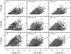 |
Fig. 16 Same as Fig. 15 for AV and M⋆. |
| In the text | |
|
Fig. 17 Relation between stellar mass and reddening for DEC+NEB model at z ~ 4. Blue dots represent galaxies with median age ≤ 107 years; red squares: 107 < age ≤ 108, yellow upward triangles: 108 < age ≤ 109 and black downward triangles: age >109 years. |
| In the text | |
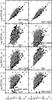 |
Fig. 18 Same as Fig. 6 for SFR. |
| In the text | |
|
Fig. 19 Distribution of the ratio t/τ at z ~ 4, with objects with age ≤50 Myr in blue, and objects with age >50 Myr in red. |
| In the text | |
|
Fig. 20 Same as Fig. 15 for M⋆ and SFR. The dashed line represents the SFR–M⋆ relation found in Daddi et al. (2007) at z ~ 2. |
| In the text | |
 |
Fig. 21 Same as Fig. 15 for specific SFR. |
| In the text | |
|
Fig. 22 Composite probability distribution of M1500 and SFR for the REF (top), DEC+NEB (centre) and RIS+NEB model (bottom) for the sample at z ~ 4 as determined for each galaxy from our 1000 Monte Carlo simulations. The overlaid points show the median value properties for each object in the sample with black dots for “weak” nebular emitters and white dots for “strong” nebular emitters. The overlaid contours indicate the 68% integrated probabilities on the ensemble properties measured from the centroid of the distribution. The dashed line represents the Kennicutt relation (Kennicutt 1998). |
| In the text | |
|
Fig. 23 Median ages are given in bin of absolute magnitude at 1500 Å (no correction for dust) from z ~ 3 to 6 for four models. Squares illustrate constant SFR with downward (upward) triangles decreasing (rising) SFHs. Black symbols stand for models without nebular emission; red symbols for models that include nebular emission (NEB), and blue symbols for NEB+Lyα. The error bars correspond to the 68% confidence limits of the probability distribution in each bin. Dashed lines show the amount of time spanned, since the previous redshift bin. |
| In the text | |
 |
Fig. 24 Same as Fig. 23 for AV. |
| In the text | |
|
Fig. 25 Same as Fig. 23 for SFR and for active galaxies (i.e. “strong” emitters). The dashed line shows the Kennicutt relation (Kennicutt 1998). |
| In the text | |
|
Fig. 26 Same as Fig. 23 for SFR and for quiescent galaxies (i.e. “weak” emitters). The dashed line shows the Kennicutt relation. |
| In the text | |
|
Fig. 27 Same as Fig. 23 for stellar mass. In each panel, we plot the M⋆–M1500 found at z ~ 4 for a more convenient comparison with other studies (Stark et al. 2009; Lee et al. 2011). Solid black line: relationship for REF model, dashed black line: REF+NEB model, dashed red line: DEC+NEB, and dash-dotted red line: RIS+NEB. |
| In the text | |
|
Fig. 28 Same as Fig. 20 for three models (top: REF, centre: DEC+NEB, bottom: RIS+NEB) at z ~ 3 (left) and z ~ 6 (right). For z ~ 6, models with declining and rising SF include Lyα. |
| In the text | |
|
Fig. 29 Median specific star formation rate as a function of redshift for four models with a 68% confidence limit based on the whole probability distribution function with comparison of results from different studies (Noeske et al. 2007; Daddi et al. 2007; Stark et al. 2009; Reddy et al. 2012b) and results from studies accounting for nebular emission effect (Stark et al. 2013; Smit et al. 2013). At z ~ 6, we show results with +NEB+Lyα option for declining and rising SFHs. Typical errors are ~ 0.3 dex. The dashed line shows the relation expected from Bouché et al. (2010) for an exponentially increasing star formation at a fixed M⋆ = 109.5 M⊙. The dotted line given by sSFR = 2 Gyr-1 is shown to guide the eye. |
| In the text | |
|
Fig. 30 Composite probability distribution of M1500 and M⋆ for REF and DEC+NEB(+Lyα) models at z ~ 5 and z ~ 6. The dashed black line represents the M⋆–M1500 trend found by González et al. (2011) and dotted black lines show a scatter of ±0.5 dex. The points overlaid show the median value properties for each object in the sample: black dots for “weak” nebular emitters, and white dots for “strong” nebular emitters. The overlaid contour indicates the 68% integrated probabilities on the ensemble properties measured from the centroid of the distribution. Red dots are median values of M⋆ in MUV bins. |
| In the text | |
Current usage metrics show cumulative count of Article Views (full-text article views including HTML views, PDF and ePub downloads, according to the available data) and Abstracts Views on Vision4Press platform.
Data correspond to usage on the plateform after 2015. The current usage metrics is available 48-96 hours after online publication and is updated daily on week days.
Initial download of the metrics may take a while.