© ESO, 2013

1. Introduction

Spectra of astronomical objects provide a wealth of information, and the increasing need for higher precision has led to the development of very stable and fibre-fed spectrographs. A prospering example is the search for exoplanets with Doppler spectroscopy. Cross-dispersed, high-resolution echelle spectrographs are usually employed to measure radial velocities at a precision of 1 m/s, which corresponds to about 1/1000 of a pixel. Therefore careful calibration, as well as high mechanical, thermal, and pressure stability, is essential.

If aiming for high precision, not only is the hardware important, but also the software algorithms to process the images. Typically, a reduction of echelle spectra consists of several steps: bias subtraction, dark subtraction, scattered light subtraction, flat-fielding, extraction to 1D, deblazing, wavelength calibration, order merging, flux normalisation (e.g. Baranne et al. 1996). In this work we focus on extraction, which is a crucial step in image processing. A widely used method is the so-called optimal extraction (Horne 1986) and its variants (e.g. Marsh 1989; Piskunov & Valenti 2002, Table 1), which basically scales 1D cross-sectional profiles to the imaged spectrum, and the scaling factor is the best flux estimate. Additionally, most algorithms try to model and reconstruct the spatial profile/slit function with polynomial, Gaussian, or other smooth functions. However, for stabilised spectrographs, the order profiles and positions are object- and time-independent, which simplifies the extraction; in particular, there is not necessarily any need to model the spatial profile with empirical functions. We exploit this circumstance, and we derive and test our concept of flat-relative optimal extraction.

2. Principle of flat-relative optimal extraction (FOX)

In the following, we assume that the image processing steps (e.g., bias, dark, and background subtraction, non-linearity correction) preceding extraction are properly done and that, in the image, the main dispersion is oriented in a more or less horizontal direction (x) and the cross-dispersion (echelle orders) in a vertical direction (y).

A spectrograph consists of dispersive elements and a camera that images the slit or the fibre exit to wavelength-dependent positions and shapes. The observed light distribution S(x,y) is a convolution of the input spectrum s(λ) with a wavelength-dependent instrumental point spread function (iPSF) of the spectrograph Ψ(x,y,λ). Therefore a model Ŝ(x,y) for the observed spectrum can be formulated as $\begin{array}{ccc}\mathit{Ŝ}\mathrm{\left(}\mathit{x,y}\mathrm{\right)}\mathrm{=}\mathrm{\Psi }\mathrm{\left(}\mathit{x,y,\lambda }\mathrm{\right)}\mathrm{\otimes }\mathit{s}\mathrm{\left(}\mathit{\lambda }\mathrm{\right)}& & \end{array}$(1)where wavelength λ and the positions x and y in the detector plane are continuous variables (the hat indicates the model or best estimate, while without the hat it indicates observations with noise: S(x,y) = Ŝ(x,y) + σ(x,y)). Furthermore, the spectrum is recorded and binned by detector pixels. Therefore it is convenient to use an effective point spread function (ePSF, Anderson & King 2000) and a discrete version of Eq. (1) as in Bolton & Schlegel (2010)$\begin{array}{ccc}\mathit{Ŝ}\mathit{x,y}\mathrm{=}\sum _{\mathit{\lambda }}{\mathrm{\Psi }}_{\mathit{x,y,\lambda }}{\mathit{s}}_{\mathit{\lambda }}& & \end{array}$(2)where x and y now correspond to pixel indices, and a finite integration over wavelength λ still has to be done. The calibration matrix Ψ_x,y,λ tabulates the effective response function of the spectrograph and detector. In Bolton & Schlegel (2010), Eq. (2) serves as model for “perfect” extraction.

Optimal extraction uses the column numbers as extraction grid (λ → x) and basically assumes 1D slit functions; i.e., any input wavelength λ that corresponds to the pixel x is imaged only to that column, meaning only pixels in the spatial direction y are affected, but no neighbouring columns. Under these circumstances the calibration matrix can be separated as $\begin{array}{ccc}{\mathrm{\Psi }}_{\mathit{x,y,\lambda }}\mathrm{=}{\mathit{\delta }}_{\mathit{x,\lambda }}{\mathit{\psi }}_{\mathit{\lambda ,y}}& & \end{array}$(3)where δ_x,λ is the Kronecker delta¹ and ψ_λ,y the wavelength-dependent cross-section. Then the model image in Eq. (2) simplifies to $\begin{array}{ccc}\mathit{Ŝ}\mathit{x,y}\mathrm{=}{\mathit{\psi }}_{\mathit{x,y}}{\mathit{s}}_{\mathit{x}}\mathit{.}& & \end{array}$(4)The response ψ_x,y could be measured directly with a uniform input spectrum s_x = 1, but it is much more challenging to determine Ψ_x,y,λ. In practice, exposures of flat lamps F_x,y are usually taken as part of regular calibration sets. Those flat exposures have high signal-to-noise ratios (S/Ns), and it can be further increased in master flats by coadding many flat exposures. This means that the errors are negligible compared to science exposures and that we can set . The spectrum of a flat lamp f_x is generally not uniform overall, but continuous and featureless, and it varies slowly with wavelength. If f_x is known, we measure the response as ${\mathit{\psi }}_{\mathit{x,y}}\mathrm{=}\frac{{\mathit{F}}_{\mathit{x,y}}}{{\mathit{f}}_{\mathit{x}}}$ directly. However, f_x is usually not known in advance and actually it cannot be measured from the flat exposure alone. It should be characterised externally, either in advance by another flux-calibrated instrument or afterwards by observations of standard stars (with known spectra) with the same instrument as part of the flux calibration step. Since both might not be available, we extract the science spectrum s_x relative to the flat spectrum f_x and write for the model $\begin{array}{ccc}\mathit{Ŝ}\mathit{x,y}\mathrm{=}{\mathit{F}}_{\mathit{x,y}}\frac{{\mathit{s}}_{\mathit{x}}}{{\mathit{f}}_{\mathit{x}}}\mathrm{·}& & \end{array}$(5)We obtain the spectrum $\frac{{\mathit{s}}_{\mathit{x}}}{{\mathit{f}}_{\mathit{x}}}$ by minimising the residuals between observations S_x,y and model Ŝ_x,y, i.e. solving the linear least-square problem $\begin{array}{ccc}{\mathit{\chi }}^{\mathrm{2}}\mathrm{\approx }\sum _{\mathit{x,y}}{\mathit{w}}_{\mathit{x,y}}{\left[{\mathit{S}}_{\mathit{x,y}}\mathrm{-}{\mathit{F}}_{\mathit{x,y}}\frac{{\mathit{s}}_{\mathit{x}}}{{\mathit{f}}_{\mathit{x}}}\right]}^{\mathrm{2}}\mathrm{=}\mathrm{minimum}& & \end{array}$(6)where w_x,y are the weights for each pixel using a noise model σ_x,y (e.g. photon and readout noise; see Sect. 3). These weights may also include a map M_x,y masking bad pixels and pixels outside the extraction aperture (${\mathit{w}}_{\mathit{x,y}}\mathrm{=}\frac{{\mathit{M}}_{\mathit{x,y}}}{{\mathit{\sigma }}_{\mathit{x,y}}^{\mathrm{2}}}$). Setting the derivative of χ² with respect to $\frac{{\mathit{s}}_{\mathit{x}}}{{\mathit{f}}_{\mathit{x}}}$ equal to zero, we get a set of decoupled equations with the solution at each position $\begin{array}{ccc}{\mathit{r}}_{\mathit{x}}\mathrm{\equiv }\frac{{\mathit{s}}_{\mathit{x}}}{{\mathit{f}}_{\mathit{x}}}\mathrm{=}\frac{{\sum }_{\mathit{y}}{\mathit{w}}_{\mathit{x,y}}{\mathit{F}}_{\mathit{x,y}}{\mathit{S}}_{\mathit{x,y}}}{{\sum }_{\mathit{y}}{\mathit{w}}_{\mathit{x,y}}{\mathit{F}}_{\mathit{x,y}}{\mathit{F}}_{\mathit{x,y}}}\hspace{0.17em}\mathit{,}& & \end{array}$(7)where $\frac{{\mathit{s}}_{\mathit{x}}}{{\mathit{fx}}_{}}$ is the best fitting amplitude at each spectral bin x. Figure 1 illustrates the principle of flat-relative optimal extraction (FOX).

Equation (7) is quite similar to the well known optimal extraction equation (e.g. Horne 1986). The difference is that we extract the spectrum s_x relative to the flat spectrum f_x, and F_x,y is not normalised and includes the natural spatial profile and all flat-field effects.

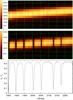Fig. 1 Principle of flat-relative optimal extraction (FOX). Each of the two upper panels shows a 400 pix × 13 pix section of the reddest HARPS order (fibre A). Pixel-to-pixel variations, fringing, order tilt/curvature, and the spatial profile are present in both the master flat Fx,y (top) and the stellar raw spectrum Sx,y which has additional (telluric) absorption lines (middle). The extracted spectrum sx / fx (bottom) is the scaling factor between both spectra for each column within the extraction mask (red lines).

3. Noise model and error estimation

The pixels on the detector (and therefore the extracted values s_x / f_x) are affected by noise σ_x,y. This consists mainly of photon noise ${\mathit{\sigma }}_{\mathrm{ph}}^{\mathrm{2}}\mathrm{=}\mathit{Ŝ}{}_{\mathit{x,y}}$ (if both σ_ph and Ŝ_x,y are in units of photon counts)² and detector noise (e.g. the readout noise ${\mathit{\sigma }}_{\mathrm{rn}}^{\mathrm{2}}$ of a CCD). Therefore, a simple noise model for each pixel is, for instance (now all units in ADU), $\begin{array}{ccc}{\mathit{\sigma }}_{\mathit{x,y}}^{\mathrm{2}}\mathrm{=}{\mathit{\sigma }}_{\mathrm{rn}}^{\mathrm{2}}\mathrm{+}\mathit{g}\mathit{Ŝ}\mathit{x,y}& & \end{array}$(8)where constant gain g (which converts the number of photoelectrons to ADU)³ and constant readout noise ${\mathit{\sigma }}_{\mathrm{rn}}^{\mathrm{2}}$ are assumed.

With a given noise model, one can predict the extraction uncertainties through error propagation of Eq. (7) $\begin{array}{ccc}\mathrm{var}\mathrm{\left(}{\mathit{r}}_{\mathit{x}}\mathrm{\right)}\mathrm{=}{\mathit{ϵ}}_{{\mathit{r}}_{\mathit{x}}}^{\mathrm{2}}& \mathrm{=}& \sum _{\mathit{y}}{\left(\frac{\mathit{\partial }{\mathit{r}}_{\mathit{x}}}{\mathit{\partial }{\mathit{S}}_{\mathit{x,y}}}\right)}^{\mathrm{2}}{\mathit{\sigma }}_{\mathit{x,y}}^{\mathrm{2}}\mathrm{=}\sum _{\mathit{y}}{\left(\frac{{\mathit{F}}_{\mathit{x,y}}\mathit{/}{\mathit{\sigma }}_{\mathit{x,y}}^{\mathrm{2}}}{{\sum }_{{\mathit{y}}^{\mathrm{\prime }}}{\mathit{w}}_{\mathit{x,}{\mathit{y}}^{\mathrm{\prime }}}{\mathit{F}}_{\mathit{x,}{\mathit{y}}^{\mathrm{\prime }}}^{\mathrm{2}}}\right)}^{\mathrm{2}}{\mathit{\sigma }}_{\mathit{x,y}}^{\mathrm{2}}\\ & \mathrm{=}& \end{array}$(9)(similar to Horne 1986). We also see that the relative error, $\begin{array}{ccc}\frac{{\mathit{ϵ}}_{{\mathit{r}}_{\mathit{x}}}}{{\mathit{r}}_{\mathit{x}}}\mathrm{=}\frac{\sqrt{{\sum }_{\mathit{y}}{\mathit{w}}_{\mathit{x,y}}{\mathit{F}}_{\mathit{x,y}}^{\mathrm{2}}}}{{\sum }_{\mathit{y}}{\mathit{w}}_{\mathit{x,y}}{\mathit{F}}_{\mathit{x,y}}{\mathit{S}}_{\mathit{x,y}}}\hspace{0.17em}\mathit{,}& & \end{array}$(10)is smaller in regions with high flux S_x,y and is scaling invariant with respect to the flat image F_x,y, because multiplying F_x,y by a constant (as happens for a longer flat exposure time) will cancel out in the ratio in Eq. (10).

The a priori predicted uncertainty in Eq. (9) does not account for the goodness of fit and thus does not indicate profile or noise model mismatches. For this reason, the error estimates from the χ² modelling are often rescaled by ${\mathit{\chi }}_{\mathrm{red}}^{\mathrm{2}}$(the reduced χ²) to provide a posteriori estimated errors $\begin{array}{ccc}{\mathit{\sigma }}_{{\mathit{s}}_{\mathit{x}}\mathit{/}{\mathit{f}}_{\mathit{x}}}\mathrm{=}{\mathit{\chi }}_{\mathrm{red}}\mathrm{·}{\mathit{ϵ}}_{{\mathit{s}}_{\mathit{x}}\mathit{/}{\mathit{f}}_{\mathit{x}}}& & \end{array}$(11)where ${\mathit{\chi }}_{\mathrm{red}}\mathrm{=}\sqrt{\frac{\mathrm{1}}{\mathit{N}\mathrm{-}\mathit{\nu }}\hspace{0.17em}{\mathit{\chi }}^{\mathrm{2}}}$ with χ² from the global fit in Eq. (6). The number of degrees of freedom N − ν in the denominator is given by the number of unmasked pixels N =  ∑ _x,yM_x,y within the extraction aperture and the number of fitted parameters ν (extracted spectral values).

One can also consider another, second choice for the scaling factor, namely χ_red,x to be taken from the individual cross-section fits, i.e. ${\mathit{\chi }}_{\mathrm{red}\mathit{,x}}^{\mathrm{2}}\mathrm{=}\frac{\mathrm{1}}{{\mathit{N}}_{\mathit{x}}\mathrm{-}\mathrm{1}}\hspace{0.17em}{\mathit{\chi }}_{\mathit{x}}^{\mathrm{2}}$ where only one free parameter is left (ν = 1), ${\mathit{\chi }}_{\mathit{x}}^{\mathrm{2}}$ is the weighted sum of the residuals only in column x and N_x =  ∑ _yM_x,y is the number of unmasked pixels in that column. However, for fibre-fed spectrographs, the extraction aperture is only a few pixels (N_x ~ 10) wide. This gives low number statistics making χ_red,x itself very uncertain (in contrast to ${\mathit{\chi }}_{\mathrm{red}}^{\mathrm{2}}$ which is approximately the average of all ${\mathit{\chi }}_{\mathrm{red}\mathit{,x}}^{\mathrm{2}}$)⁴. In particular, a considerable number of χ_red,x will occur with values much less than one, when fitting the profiles along the dispersion axis. However, the predicted errors should not be smaller than the fundamental limit (e.g. photon noise).

As discussed in Horne (1986), cosmic ray hits can be efficiently detected and removed with optimal extraction. Those cosmics distort the profile and can be identified as significant outliers by means of the noise model, e.g. by setting an upper threshold $\begin{array}{ccc}{\mathit{S}}_{\mathit{x,y}}\mathrm{-}\mathit{Ŝ}\mathit{x,y}\mathit{>}\mathit{\kappa }\sqrt{\mathrm{var}\mathrm{(}{\mathit{S}}_{\mathit{x,y}}\mathrm{-}\mathit{Ŝ}\mathit{x,y}\mathrm{)}}\mathrm{=}\mathit{\kappa }\mathrm{·}\mathrm{(}{\mathit{\sigma }}_{\mathit{x,y}}^{\mathrm{2}}\mathrm{-}{\mathit{F}}_{\mathit{x,y}}^{\mathrm{2}}{{\mathit{ϵ}}_{{\mathit{s}}_{\mathit{x}}\mathit{/}{\mathit{f}}_{\mathit{x}}}^{\mathrm{2}}}^{\mathrm{)}}\mathit{,}& & \end{array}$(12)(see Appendix A for a derivation of this equation), where the clipping value is typically κ ~ 3 − 5 to reject cosmics. A lower threshold could be set as well, e.g. to detected unmasked cold pixels. Moreover, other or additional criteria are also used (Baranne et al. 1996). The outliers are masked and the extraction process is repeated.

We note that the variance in the residual image S_x,y − Ŝ_x,y is generally not just the pixel variance ${\mathit{\sigma }}_{\mathit{x,y}}^{\mathrm{2}}$. In contrast to Horne (1986) the correction term ${\mathit{F}}_{\mathit{x,y}}^{\mathrm{2}}{\mathit{ϵ}}_{{\mathit{s}}_{\mathit{x}}\mathit{/}{\mathit{f}}_{\mathit{x}}}^{\mathrm{2}}$ should be applied in Eq. (12). Figuratively, the observed dispersion in the residuals will be noticeably smaller than ${\mathit{\sigma }}_{\mathit{x,y}}^{\mathrm{2}}$, because the number of pixels within the aperture is, as already mentioned, small and the profile is usually not uniform, but concentrates most flux in even fewer pixels (~3–4 pixels in fibre-fed spectrographs). Imagine a concentrated profile, where one pixel has a very high weight. This pixel dominates the fit, thus forcing its own residual to zero. As an example, in Fig. 1 the pixel in the profile centre contains about 25% of the total profile flux, and the observed dispersion in this pixel will be smaller than σ_x,y by a factor of 0.56 in case of readout dominated noise (Eq. (A.16)) and by 0.75 in case of pure photon noise (Eq. (A.17)).

4. Conceptual comparison with other optimal extraction implementations

Numerous optimal extraction algorithms (hereafter OXT) exists that are listed in Table 1. Usually, they have to assume a slowly varying spatial profile and differ in the reconstruction method for this profile. Using the spatial profiles of many columns, a mean high S/N model is created. Since OXT aims to estimate “absolute” counts⁵, the profile functions p_x,y are normalised to unity (∑ _yp_x,y = 1).

If there is no or slow order tilt, the profile might be reconstructed by averaging (Hewett et al. 1985) or fitting low-order polynomials in the dispersion direction (Horne 1986), respectively. For echelle spectrographs, this situation occurs only in small sections of the orders, but not in general. For larger tilts, the order trace (which describes the vertical position of the profile along the x direction) appears more or less explicitly in the profile modelling, and sub-pixel grids are introduced. Then neighbouring polynomials in dispersion direction are coupled (Marsh 1989), or recentred cross-sections are fitted by smoothing (spline-like) functions (Piskunov & Valenti 2002; Bolton & Burles 2007). Those algorithms need a good description of the trace to properly position the profile model. In particular, for order regions grazing the detector borders, the order tracing and the application of OXT algorithms is difficult.

An advantage of OXT is that the profile reconstruction can be done on the object spectrum itself. This is crucial for slit spectrographs where the shape and position of the object on the slit and/or detector can be different in the next exposure or change even during an exposure, depending on the seeing, guiding, and temperature. The noise in the mean profiles is then reduced by about the square root of the number of used columns compared to individual profiles (assuming an absorption spectrum; however, this approach may have problems with emission line spectra that have profile information only in a few columns).

The concept of optimal extraction was originally developed for slit spectrographs, and the application to fibre-fed spectrographs seemed natural. If the image shape becomes insensitive to seeing and guiding (as for fibre-fed instruments), one can save the effort of the profile modelling on the object itself (which can become computationally extensive as in Piskunov & Valenti 2002) and a less noisy reference profile model might be taken from a reference image or a flat (Marsh 1989; Baranne et al. 1996). Still, a recentring of the model might be needed to account for sub-pixel shifts (e.g. a nightly shift of 0.1 pixels was reported by Baranne et al. for ELODIE).

If additionally the position of the image is fixed, as for stabilised instruments without mechanical and thermal flexure, then recentring also becomes redundant. In this case there is even no longer any need to model the profile that now can be taken directly from the flat, therefore FOX does not require any choices for model parameters such as the polynomial degree, the subpixel grid size, or the amount of smoothing.

Another benefit of the fixed format is that flat-field effects can be included in the extraction mask, and in this sense FOX does the flat-fielding simultaneously. Also from Eq. (7), we note that there is no need for a pixel-wise division by a flat (an operation one likes to avoid, especially when small numbers occur as in the wings of the cross-sections).

The classical data reduction with OXT requires an additional pre- and/or post-flat-fielding, i.e. before and/or after extraction (Baranne et al. 1996). Flat-fielding has the task of correcting for various multiplicative efficiency effects that have various causes and scales. Locally, there are, e.g., pixel-to-pixel variations owing to different sizes and quantum efficiencies of the detector pixels. Fringe patterns are interference effects that become serious in the red orders and depend on the properties of CCD (layer thickness) and the incident light (wavelength, angle, position). The blaze efficiency along and across the orders depends on the echelle grating and the cross-disperser. Finally, there is also a wavelength-dependent efficiency of the detector and optical elements (e.g. fibre transmission). We may summarise these effects as ε_x,y = ε_pixel,x,y ε_fringe,x,y ε_blaze,x ε_λ,x.

Basically, ε_blaze and ε_λ are only functions of x and they could be corrected after extraction. However, ε_pixel and ε_fringe have spatial components and should be corrected before (or, as in FOX, during) the extraction. If not, the profile mismatches result in less correct flux estimates, and in particular, residing fringe patterns lead to strong, rapid, and systematic profile variations violating the above assumption as needed for the profile modelling.

Data reduction pipelines using OXT create a normalised flat-field image. Those might be obtained as part of the decomposition of flat exposure into a normalised flat image, a normalised profile/order shape, and the blaze function (Piskunov & Valenti 2002). Another technical approach is to use, if existing, wider or moving fibres to get a uniform illumination (similar to a long-slit, Baranne et al. 1996), but fringe patterns are likely not properly captured.

5. FOX in action

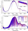Fig. 2 Spectra of HD 60753 and τ Cet extracted with FOX. The orders (alternating colours) are not merged. The spectrum is not flux-corrected, but is relative to the spectrum of the flat lamp. The inset shows the overlap between two orders.

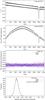Fig. 3 Comparison of the extraction quality for two HARPS spectra of the B3IV star HD 60753 taken in the same night (S / N ~ 170). Top: extraction with FOX. Second panel: spectrum extracted with the HARPS DRS pipeline (not blaze corrected). Third panel: ratio of both exposures for FOX (red dots) and DRS (blue dots). Bottom: histogram of the ratio values. The black line is a Gaussian fit to the FOX histogram having a centre at 0.914 and a width of 0.00905.

To demonstrate the performance of FOX, we extract spectra taken with HARPS, an echelle spectrograph at the 3.6 m ESO telescope in La Silla (Chile), located in a pressure- and temperature-stabilised vacuum tank (Mayor et al. 2003). It is fed by two fibres from the Cassegrain focus, a science fibre (A) and a calibration fibre (B) to simultaneously monitor wavelength drift or sky background. HARPS has a resolving power of R = 110 000 and covers the wavelength range 3800–6900 Å with 72 orders (fibre A) on a 4 k × 4 k CCD. Figure 1 shows a section of a HARPS raw spectrum.

We also choose HARPS observations, because there is an elaborated pipeline for HARPS called data reduction software (DRS, version 3.5)⁶ that already has demonstrated high performance and allows comparison to our extraction results. The DRS employs the Horne (1986) algorithm and since version 3.5 uses coadded flat-fields to define the extraction profile (C. Lovis, Observatoire de Genève, priv. comm.). It is here supposed to represent optimal extraction. Both the raw and reduced spectra are publicly available⁷.

We extracted spectra for a standard star (HD 60753, B3IV) and a solar-like star (τ Cet, G8V). We used the REDUCE package of Piskunov & Valenti (2002) for the preprocessing: the bias frames were averaged to a master bias; five flat exposures were bias-subtracted, averaged to a master flat and the scattered light was subtracted; one order-location frame (a flat lamp illuminating only fibre A) was used to define the order traces of fibre A; from the science images, the master bias and the scattered light were subtracted (no pre-flat-fielding was performed). Then we extracted the science spectra with our FOX algorithm with a spatial extraction width of ten pixels (five whole pixels below and five above the order trace), σ_rn = 5 ADU, and $\mathit{g}\mathrm{=}\mathrm{0.70}\hspace{0.17em}\mathrm{ADU}\mathit{/}{\mathrm{e}}_{\mathrm{ph}}^{\mathrm{-}}$. The wavelength solutions were taken from the DRS pipeline.

Figure 2 shows the result of the FOX extraction for two observations. As can be seen, the extracted orders match in the overlapping regions and seem to be ready to be merged directly. Order merging, however, is not the topic of this work and is not necessary for our RV computations below. Merging also needs some care, since the different resolution and sampling will lead to mismatches in the absorption and emission features, and in this way some information is also lost.

5.1. S/N measurement for the standard star

To measure the extraction quality, we use two observations of the standard star HD 60753, taken three hours apart in the night 2007-03-26; exposures times 9.5 min, and various methods of estimating S/Ns. Figure 3 displays the extracted aperture number 68 (6613–6687 Å) of the standard star (the prominent absorption line is He I).

Using the uncertainties derived from the noise model (Eq. (9)), we estimate for FOX a quadratic mean signal-to-noise of $\mathit{S}\mathit{/}\mathit{N}\mathrm{=}\sqrt{\frac{\mathrm{1}}{\mathit{n}}{\sum }_{\mathit{x}}\frac{{\mathit{r}}_{\mathit{x}}^{\mathrm{2}}}{{\mathit{ϵ}}_{{\mathit{r}}_{\mathit{x}}}^{\mathrm{2}}}}\mathrm{=}\mathrm{169.6}$ (exposure 2: 176.9) per extracted pixel around the central n = 100 pixels. Since no uncertainties are provided for DRS spectra, we assume pure photon noise (${\mathit{ϵ}}_{\mathit{x}}\mathrm{=}\sqrt{{\mathit{s}}_{\mathit{x}}}$). Then the count level in the DRS spectrum implies a mean photon S/N of $\sqrt{⟨{\mathit{s}}_{\mathit{x}}⟩}\mathrm{=}\mathrm{170.4}$ (exposure 2: 178.6)⁸. These S/N values are similar and provide fundamental limits. In this respect, we note that we have χ_red = 1.08 for this order.

Another way to measure the S/N independently of a priori error estimates is to analyse the scatter in a continuum region. (This is the reason for choosing a standard star for the comparison.) For the same central region, the S/N per extracted pixel derived as the ratio of the intensity mean and the standard deviation ($\mathit{S}\mathit{/}\mathit{N}\mathrm{=}\frac{{}_{\mathrm{⟨}}\mathit{s}_{\mathit{x}}{}_{\mathrm{⟩}}}{⟨\mathrm{(}{\mathit{s}}_{\mathit{x}}\mathrm{-}⟨{\mathit{s}}_{\mathit{x}}⟩{\mathrm{)}}^{\mathrm{2}}⟩}$) is 185 (exposure 2: 163) for FOX and 177 (exposure 2: 141) for DRS. These numbers already indicate that the extraction qualities are similar.

In a further comparison (also independent of a priori error estimates), we take the ratio of the two spectra of the standard star and analyse the scatter. Taking the ratio of both spectra cancels out the remaining flat spectrum in the case of FOX and the blaze function in the case of DRS, therefore allowing for a more direct comparison over a wider range and even pixel-wise. We see in the third panel of Fig. 3 that the ratio values of FOX (q_x = r_x,exp1 / r_x,exp2) and DRS (q_x = s_x,exp1 / s_x,exp2) have a similar mean (~0.914, constant over the full order) and are correlated. For both extractions, the scatter appears similar and barely distinguishable by eye. In both cases the scatter increases towards the order edges (since the flux decreases due to the blaze, see second panel of Fig. 3). As before, we measured a S/N from the mean and the standard deviation of the ratio values for the central 100 pixels and find a slightly higher S/N for FOX (S / N_q,FOX = 133 and S / N_q,DRS = 129).

In contrast to the previous method, we can extend this ratio method over the full order and also use regions with stellar lines (assuming that the stellar lines are static, i.e. do not vary in shape and position). A slight, relative shift between both spectra is present owing to the difference in their barycentric radial velocities (212 m/s, ~0.25  pix). The slightly increased scatter noticeable at the position of the strong stellar line is due to this shift as well as to the lower flux level (lower S/N).

The last panel of Fig. 3 shows a histogram for the 4096 ratio values. We see that the ratio values have nearly a Gaussian distribution, and we now measure the mean and dispersion more robustly from a Gaussian fit to the histograms. Using ${\mathrm{S}\mathit{/}\mathrm{N}}_{\mathit{q}}\mathrm{=}\frac{\mathit{\mu }}{\mathit{\sigma }}$, we find values of 100.77 (FOX) and 100.87 (DRS) for order 68. The same procedure was applied to the other orders and the results plotted in Fig. 4. The overall course of the S / N_q values mostly reflects the instrument efficiency (times the stellar energy distribution) along the order. Both FOX and DRS extraction deliver similar S / N_q with quotients close to unity and deviation of ≲1%, whereas in this example FOX provided slightly higher S/N in the blue orders.

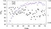Fig. 4 Signal-to-noise S / Nq measured in the spectrum ratio qx of two standard star exposures for several orders from the extraction FOX (red plus) and DRS (blue crosses). The quotient of the S/N values between FOX and DRS (black filled circles) refer to the right axis and are close to unity.

5.2. RV performance for a Sun-like star

As a further, less direct, but probably more relevant proxy for the extraction quality we use radial velocity (RV) measurements. The RV precision depends on the S/N in the observation and the RV information content of the stellar spectral lines (the number and amount of gradients; Bouchy et al. 2001). In particular this means that we are probing the extraction quality in the flanks of spectral lines (rather than in continuum regions as before).

We have chosen an asteroseismology run from the night 2004-10-02 for the star Tau Cet, which is a known RV standard with a dispersion at the 1 m/s level over years (Pepe et al. 2011). This night provides the large number (438) of spectra needed to visualise the close performance of FOX and DRS (Fig. 5). Since all data were taken during the same night, we can defer discussions about the systematics due to the wavelength calibration, which is another crucial step in data reduction.

For the RV measurements we use the method of least-square template matching (Anglada-Escudé & Butler 2012). The RVs are measured over several orders, the ten bluest orders, as well as regions contaminated by telluric absorptions features have been excluded. The top panel in Fig. 5 shows that RV differences resulting from the FOX and DRS extraction are small and at or below the 1 m/s level. The rms is 1.50 m/s with FOX and 1.49 m/s with DRS extraction. Since the DRS pipeline also delivers high-quality RVs measured by cross-correlation with a binary template, we provide a comparison in the lower panel of Fig. 5 showing the impact of using the same extraction method (DRS) but a different RV computation.

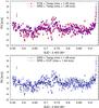Fig. 5 Radial velocities of τ Cet in the night of 2004-10-02 computed with the least square method for FOX and DRS extraction (top) and for comparison the radial velocities from cross-correlation for DRS extraction (bottom).

The two examples presented in this section demonstrate that the concept of FOX can work in practice and indicate that FOX has a similar and comparable performance in terms of S/N and RV precision compared to standard optimal extraction.

6. Limits of optimal extraction

FOX and other optimal extraction algorithms assume 1D slit functions that are aligned with the detector columns. However, in practice the slit or fibre image is usually resolved and sampled by a few pixels in the spatial and dispersion direction, and the injection of a monochromatic wavelength causes a 2D PSF that can be seen in emission line spectra. We investigate this effect in data from HARPS.

Figure 6 shows the sharp features of a spectrum from a laser frequency comb (LFC; Murphy et al. 2007; Wilken et al. 2010) observed with HARPS (order 44). The residuals of the extraction (S_x,y − Ŝ_x,y) are shown in the lower panel, where Ŝ_x,y is computed with the extracted spectrum r_x and Eq. (5)). Of course, the residuals are larger in regions with larger flux (more photon noise). However, a systematic (not random) pattern remains: the residuals are always too low in the peak centre (by ~10%!) and too high up left, as well as down right from the peak centres (this pattern is also similar to the simulation of Bolton & Schlegel 2010; see their Fig. 1). The reason for this pattern is the mismatch between the individual 2D PSF cross-sections and flat-field cross-profiles (which could be thought of as the 2D PSF cross-sections integrated along the disperion axis). Only if the individual 2D PSF cross-sections were self-similar would the mismatch diminish.

We visualise some cross-sections in Fig. 7 at the positions indicated in Fig. 6. This region was selected because the order tilt is small and the LFC peak distances are close to integer values (multiple of 12.0 pixels), i.e. the LFC peaks have only small pixel phase shifts here and samples similar phases of the effective PSF. Each of the 18 profiles (3 cuts for each of the 6 peaks) is normalised to unit area. Obviously the profiles in the flanks have a different form (more peaky and shifted) with respect to the peak centres. The mismatches can be at the 10% level for sharp features (while they are not visible in the flat-field cross-sections taken at the same positions). This will lead to high χ_red-values in optimal extraction and biased extracted spectrum values in sharp, high S/N features.

The visible, systematic residual tilts in Fig. 6 from bottom left to top right results from an asymmetry in the PSF, although the PSF appears like a symmetric 2D Gaussian at first glance. We presume that the physical explanation for this asymmetry (present everywhere on the detector) lies in the quasi Littrow mode configuration, i.e. the usage of R4 echelle grating with an off-plane angle of 1.5° that amplifies by a factor of ≈8 to a spectral line tilt or shear (Hearnshaw 2009) and deforms the circularly symmetric image of the fibre exit.

The shortcoming of “optimal” extraction might be solved with “perfect” extraction that involves a 2D PSF as outlined in Bolton & Schlegel (2010). It can theoretically also deal with stray light and ghost features. However, besides the increased computational effort, the main problem in practice is to obtain the calibration matrix Ψ_x,y,λ.

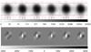Fig. 6 Section of a HARPS laser frequency spectrum Sx,y (top, logarithmic intensity scale) and residuals Sx,y − Ŝx,y after the FOX extraction (bottom, linear scale). Coloured ticks indicate positions of cross-section cuts (see Fig. 7).

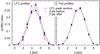Fig. 7 Cross-sections at different positions in the laser frequency comb spectrum and flat-field image. The cut positions are at the LFC peak maximum (black asterisks), two pixels before (blue crosses), and two pixels after (red plus), as indicated by the corresponding colored ticks in Fig. 6; the coloured lines connect the corresponding profile means. The profiles are normalised to unit area.

7. Conclusion

We have introduced a method extracting 1D spectra from 2D raw data using flat-field exposures as a measure of the instrumental profile. This method is similar to standard optimum extraction. It does not make any assumptions about the instrumental profile but requires its temporal stability between flat-field and science exposures. The method is well suited to stabilised fibre-fed spectrographs optimised for high-precision radial velocity work.

One of the main advantages of FOX is that the reconstruction of the instrumental PSF becomes unnecessary. Modelling of the PSF is a time-consuming step, and in regions of low signal, the PSF is often ill-defined in science exposures. It is therefore a strong advantage to take the PSF from well-defined flat-field exposures, which is the main idea of FOX. Following this scheme, extraction, masking, flat-fielding, and blaze correction are all carried out in one step without any need for data fitting when the calibration matrix is constructed. The decrease in required CPU time is significant, which is particularly relevant for large surveys like HARPS and CARMENES (Quirrenbach et al. 2012). Furthermore, FOX has no requirements concerning the spectral format (such as slowly varying spatial profiles), relaxes the need for accurate localisation of spectral orders, and does not involve any numerical unstable operations like division by the flat-field.

We compared the performance of FOX to standard optimal extraction using HARPS data and the HARPS data reduction system. The results are very similar with insignificant differences in the S/N. The spectra of individual orders extracted with FOX match well in the overlap regions showing that the inherent blaze correction works. We computed the RV series from HARPS spectra extracted with FOX and DRS and find them indistinguishable in terms of their rms scatter. We conclude that FOX is a highly efficient and very robust method for extracting astronomical spectroscopic data observed with stabilised fibre-fed spectrographs. FOX cannot overcome the limitations caused by tilted PSFs, stray light, or ghost features, but it can significantly improve the robustness and time efficiency of existing and future data reduction procedures.

Acknowledgments

M.Z. acknowledges support by the European Research Council under the FP7 Starting Grant agreement number 279347. We thank the referee, N. Piskunov, for many useful comments. We are also thankful to C. Lovis and G. Lo Curto for helpful discussions about the HARPS instrument and F. Bauer for reading the manuscript.

References

Appendix A: Appendix A

To estimate for each pixel the residual variance, $\begin{array}{ccc}\mathrm{var}\mathrm{(}{\mathit{S}}_{\mathit{x,y}}\mathrm{-}\mathit{Ŝ}\mathit{x,y}\mathrm{)}\mathrm{=}\mathrm{var}\mathrm{\left(}{\mathit{S}}_{\mathit{x,y}}\mathrm{\right)}\mathrm{+}\mathrm{var}\mathrm{\left(}\mathit{Ŝ}\mathit{x,y}\mathrm{\right)}\mathrm{-}\mathrm{2}\mathrm{cov}\mathrm{\left(}{\mathit{S}}_{\mathit{x,y}}\mathit{,}\mathit{Ŝ}\mathit{x,y}\mathrm{\right)}\mathit{,}& & \end{array}$(A.13)we need the pixel variance, which is $\mathrm{var}\mathrm{\left(}{\mathit{S}}_{\mathit{x,y}}\mathrm{\right)}\mathrm{=}{\mathit{\sigma }}_{\mathit{x,y}}^{\mathrm{2}}\mathrm{=}\frac{\mathrm{1}}{{\mathit{w}}_{\mathit{x}\mathit{.}\mathit{y}}}$, and an expression for the model Ŝ_x,y. Inserting Eqs. (7) and (9) into Eq. (5) gives $\begin{array}{ccc}\mathit{Ŝ}\mathit{x,y}\mathrm{=}{\mathit{F}}_{\mathit{x,y}}{\mathit{r}}_{\mathit{x}}\mathrm{=}{\mathit{F}}_{\mathit{x,y}}{\mathit{ϵ}}_{{\mathit{r}}_{\mathit{x}}}^{\mathrm{2}}\sum _{\mathit{y}}{\mathit{w}}_{\mathit{x,y}}{\mathit{F}}_{\mathit{x,y}}{\mathit{S}}_{\mathit{x,y}}\hspace{0.17em}\mathit{.}& & \end{array}$(A.14)We see that S_x,y itself contributes to Ŝ_x,y and a covariance term will persist. Assuming that the pixels are otherwise independent,

the variance of the residuals is given by $\begin{array}{ccc}\mathrm{var}\mathrm{(}{\mathit{S}}_{\mathit{x,y}}\mathrm{-}\mathit{Ŝ}\mathit{x,y}\mathrm{)}& \mathrm{=}& {\mathit{\sigma }}_{\mathit{x,y}}^{\mathrm{2}}\mathrm{+}{\mathit{F}}_{\mathit{x,y}}^{\mathrm{2}}\mathrm{var}\mathrm{\left(}{\mathit{r}}_{\mathit{x}}\mathrm{\right)}\mathrm{-}\mathrm{2}{\mathit{F}}_{\mathit{x,y}}^{\mathrm{2}}{\mathit{ϵ}}_{{\mathit{r}}_{\mathit{x}}}^{\mathrm{2}}{\mathit{w}}_{\mathit{x,y}}{\mathit{\sigma }}_{\mathit{x,y}}^{\mathrm{2}}\\ & \mathrm{=}& \end{array}$(A.15)This equation can be simplified for three special cases.

• Case 1. For pixelswith relatively low profile weights(${\mathit{F}}_{{}_{\mathit{x,y}}}^{\mathrm{2}}{\mathit{ϵ}}_{{\mathit{r}}_{\mathit{x}}}^{\mathrm{2}}\mathrm{\ll }{\mathit{\sigma }}_{\mathit{x,y}}^{\mathrm{2}}$), e.g. in the wings of spatial profiles, the residual variance just becomes ${\mathit{\sigma }}_{\mathit{x,y}}^{\mathrm{2}}$.

• Case 2. When the pixel variance is the same for all pixels σ_x,y = σ₀, e.g. readout noise dominates, we have (${\mathit{ϵ}}_{{\mathit{r}}_{\mathit{x}}}^{\mathrm{2}}\mathrm{=}{\mathit{\sigma }}_{\mathrm{0}}^{\mathrm{2}}\frac{\mathrm{1}}{\sum {\mathit{F}}_{\mathit{x,y}}^{\mathrm{2}}}$) $\begin{array}{ccc}{\mathrm{var}\mathrm{(}{\mathit{S}}_{\mathit{x,y}}\mathrm{-}\mathit{Ŝ}\mathit{x,y}\mathrm{)}|}_{{\mathit{\sigma }}_{\mathit{x,y}}\mathrm{=}{\mathit{\sigma }}_{\mathrm{0}}}& & \mathrm{=}\left[\mathrm{1}\mathrm{-}\frac{{\mathit{F}}_{\mathit{x,y}}^{\mathrm{2}}}{\sum {\mathit{F}}_{\mathit{x,y}}^{\mathrm{2}}}\right]{\mathit{\sigma }}^{\mathrm{2}}\mathrm{·}\end{array}$(A.16)Moreover, for a uniform profile (F_x,y = 1) the factor in the bracket becomes $\frac{\mathit{N}\mathrm{-}\mathrm{1}}{\mathit{N}}$ (a well known correction factor for the unbiased variance).

• Case 3. Assuming ${\mathit{\sigma }}_{\mathit{x,y}}^{\mathrm{2}}\mathrm{=}\mathit{g}\mathit{Ŝ}{}_{\mathit{x,y}}\mathrm{=}\mathit{g}{\mathit{r}}_{\mathit{x}}{\mathit{F}}_{\mathit{x,y}}$, i.e. photon noise dominates, we find $\left({\mathit{ϵ}}_{{\mathit{r}}_{\mathit{x}}}^{\mathrm{2}}\mathrm{=}\frac{\mathrm{1}}{{\sum }_{\mathit{y}}{\mathit{F}}_{\mathit{x,y}}}\mathit{g}{\mathit{r}}_{\mathit{x}}\mathrm{=}\frac{\mathrm{1}}{{\sum }_{\mathit{y}}{\mathit{F}}_{\mathit{x,y}}}\frac{{\mathit{\sigma }}_{\mathit{x,y}}^{\mathrm{2}}}{{\mathit{F}}_{\mathit{x,y}}}\right)$$\begin{array}{ccc}{\mathrm{var}\mathrm{(}{\mathit{S}}_{\mathit{x,y}}\mathrm{-}\mathit{Ŝ}\mathit{x,y}\mathrm{)}|}_{{\mathit{\sigma }}_{\mathit{x,y}}^{\mathrm{2}}\mathrm{=}\mathit{g}\mathit{Ŝ}\mathit{x,y}}& & \mathrm{=}\left[\mathrm{1}\mathrm{-}\frac{{\mathit{F}}_{\mathit{x,y}}}{\sum {\mathit{F}}_{\mathit{x,y}}}\right]{\mathit{\sigma }}_{\mathit{x,y}}^{\mathrm{2}}\hspace{0.17em}\mathit{.}\end{array}$(A.17)Again for a uniform profile the prefactor becomes $\frac{\mathit{N}\hspace{0.17em}\mathrm{-}\hspace{0.17em}\mathrm{1}}{\mathit{N}}\mathrm{·}$

All Tables

All Figures

Fig. 1 Principle of flat-relative optimal extraction (FOX). Each of the two upper panels shows a 400 pix × 13 pix section of the reddest HARPS order (fibre A). Pixel-to-pixel variations, fringing, order tilt/curvature, and the spatial profile are present in both the master flat Fx,y (top) and the stellar raw spectrum Sx,y which has additional (telluric) absorption lines (middle). The extracted spectrum sx / fx (bottom) is the scaling factor between both spectra for each column within the extraction mask (red lines).

In the text

	Fig. 2 Spectra of HD 60753 and τ Cet extracted with FOX. The orders (alternating colours) are not merged. The spectrum is not flux-corrected, but is relative to the spectrum of the flat lamp. The inset shows the overlap between two orders.
In the text

Fig. 3 Comparison of the extraction quality for two HARPS spectra of the B3IV star HD 60753 taken in the same night (S / N ~ 170). Top: extraction with FOX. Second panel: spectrum extracted with the HARPS DRS pipeline (not blaze corrected). Third panel: ratio of both exposures for FOX (red dots) and DRS (blue dots). Bottom: histogram of the ratio values. The black line is a Gaussian fit to the FOX histogram having a centre at 0.914 and a width of 0.00905.

In the text

	Fig. 4 Signal-to-noise S / Nq measured in the spectrum ratio qx of two standard star exposures for several orders from the extraction FOX (red plus) and DRS (blue crosses). The quotient of the S/N values between FOX and DRS (black filled circles) refer to the right axis and are close to unity.
In the text

	Fig. 5 Radial velocities of τ Cet in the night of 2004-10-02 computed with the least square method for FOX and DRS extraction (top) and for comparison the radial velocities from cross-correlation for DRS extraction (bottom).
In the text

	Fig. 6 Section of a HARPS laser frequency spectrum Sx,y (top, logarithmic intensity scale) and residuals Sx,y − Ŝx,y after the FOX extraction (bottom, linear scale). Coloured ticks indicate positions of cross-section cuts (see Fig. 7).
In the text

	Fig. 7 Cross-sections at different positions in the laser frequency comb spectrum and flat-field image. The cut positions are at the LFC peak maximum (black asterisks), two pixels before (blue crosses), and two pixels after (red plus), as indicated by the corresponding colored ticks in Fig. 6; the coloured lines connect the corresponding profile means. The profiles are normalised to unit area.
In the text

References

- Anderson, J., & King, I. R. 2000, PASP, 112, 1360 [NASA ADS] [CrossRef] [Google Scholar]
- Anglada-Escudé, G., & Butler, R. P. 2012, ApJS, 200, 15 [NASA ADS] [CrossRef] [Google Scholar]
- Baranne, A., Queloz, D., Mayor, M., et al. 1996, A&AS, 119, 373 [NASA ADS] [CrossRef] [EDP Sciences] [Google Scholar]
- Bolton, A. S., & Burles, S. 2007, New J. Phys., 9, 443 [NASA ADS] [CrossRef] [Google Scholar]
- Bolton, A. S., & Schlegel, D. J. 2010, PASP, 122, 248 [NASA ADS] [Google Scholar]
- Bouchy, F., Pepe, F., & Queloz, D. 2001, A&A, 374, 733 [NASA ADS] [CrossRef] [EDP Sciences] [Google Scholar]
- Hearnshaw, J. 2009, Astronomical Spectrographs and their History (Cambridge University Press) [Google Scholar]
- Hewett, P. C., Irwin, M. J., Bunclark, P., et al. 1985, MNRAS, 213, 971 [NASA ADS] [CrossRef] [Google Scholar]
- Horne, K. 1986, PASP, 98, 609 [NASA ADS] [CrossRef] [EDP Sciences] [Google Scholar]
- Marsh, T. R. 1989, PASP, 101, 1032 [NASA ADS] [CrossRef] [Google Scholar]
- Mayor, M., Pepe, F., Queloz, D., et al. 2003, The Messenger, 114, 20 [NASA ADS] [Google Scholar]
- Murphy, M. T., Udem, T., Holzwarth, R., et al. 2007, MNRAS, 380, 839 [NASA ADS] [CrossRef] [Google Scholar]
- Pepe, F., Lovis, C., Ségransan, D., et al. 2011, A&A, 534, A58 [NASA ADS] [CrossRef] [EDP Sciences] [Google Scholar]
- Piskunov, N. E., & Valenti, J. A. 2002, A&A, 385, 1095 [NASA ADS] [CrossRef] [EDP Sciences] [Google Scholar]
- Quirrenbach, A., Amado, P. J., Seifert, W., et al. 2012, in Proc. SPIE, 8446, 33 [Google Scholar]
- Robertson, J. G. 1986, PASP, 98, 1220 [NASA ADS] [CrossRef] [Google Scholar]
- Urry, M., & Reichert, G. 1988, NASA IUE Newsletter, 34, 96 [Google Scholar]
- Wilken, T., Lovis, C., Manescau, A., et al. 2010, in Proc. SPIE, 7735, 28 [Google Scholar]