| Issue |
A&A
Volume 561, January 2014
|
|
|---|---|---|
| Article Number | A5 | |
| Number of page(s) | 13 | |
| Section | Stellar structure and evolution | |
| DOI | https://doi.org/10.1051/0004-6361/201322578 | |
| Published online | 17 December 2013 | |
The wind of W Hydrae as seen by Herschel
I. The CO envelope⋆
1 Astronomical Institute Anton Pannekoek, University of Amsterdam, PO Box 94249, 1090 GE, Amsterdam, The Netherlands
e-mail: theokhouri@gmail.com
2 Instituut voor Sterrenkunde, KU Leuven, Celestijnenlaan 200D 2401, 3001 Leuven, Belgium
3 SRON Netherlands Institute for Space Research, Sorbonnelaan 2, 3584 CA Utrecht, The Netherlands
4 RAL Space, Rutherford Appleton Laboratory, Chilton, Didcot, Oxfordshire OX11 0QX, UK
5 Dept. of Physics & Astronomy, University College London, Gower St., London WC1E 6BT, UK
6 Observatorio Astronómico Nacional (IGN), Alfonso XII No 3, 28014 Madrid, Spain
7 Department of Physics and Astrophysics, Vrije Universiteit Brussel, Pleinlaan 2, 1050 Brussels, Belgium
8 Observatorio Astronómico Nacional (OAN-IGN), Apartado 112, 28803 Alcalá de Henares, Spain
9 Centro de Astrobiología (CSIC/INTA), Ctra. de Torrejón a Ajalvir, km 4, 28850 Torrejón de Ardoz, Madrid, Spain
10 Koninklijke Sterrenwacht van België, Ringlaan 3, 1180 Brussels, Belgium
11 Onsala Space Observatory, Dept. of Earth and Space Sciences, Chalmers University of Technology, 43992 Onsala, Sweden
12 University of Vienna, Department of Astrophysics, Türkenschanzstraße 17, 1180 Wien, Austria
13 European Southern Observatory, Karl Schwarzschild Str. 2, 85748 Garching bei München, Germany
14 European Space Astronomy Centre, Urb. Villafranca del Castillo, PO Box 50727, 28080 Madrid, Spain
15 Harvard-Smithsonian Center for Astrophysics, Cambridge MA 02138, USA
16 Max-Planck-Institut für Radioastronomie, auf dem Hügel 69, 53121 Bonn, Germany
17 Department of Astronomy, AlbaNova University Center, Stockholm University, 10691 Stockholm, Sweden
18 Institute for Space Imaging Science, University of Lethbridge, 4401 University Drive, Lethbridge, Alberta T1J 1B1, Canada
19 N. Copernicus Astronomical Center, Rabiańska 8, 87-100 Toruń, Poland
Received: 30 August 2013
Accepted: 3 October 2013
Context. Asymptotic giant branch (AGB) stars lose their envelopes by means of a stellar wind whose driving mechanism is not understood well. Characterizing the composition and thermal and dynamical structure of the outflow provides constraints that are essential for understanding AGB evolution, including the rate of mass loss and isotopic ratios.
Aims. We characterize the CO emission from the wind of the low mass-loss rate oxygen-rich AGB star W Hya using data obtained by the HIFI, PACS, and SPIRE instruments on board the Herschel Space Observatory and ground-based telescopes. 12CO and 13CO lines are used to constrain the intrinsic 12C/13C ratio from resolved HIFI lines.
Methods. We combined a state-of-the-art molecular line emission code and a dust continuum radiative transfer code to model the CO lines and the thermal dust continuum.
Results. The acceleration of the outflow up to about 5.5 km s-1 is quite slow and can be represented by a β-type velocity law with index β = 5. Beyond this point, acceleration up the terminal velocity of 7 km s-1 is faster. Using the J = 10–9, 9–8, and 6–5 transitions, we find an intrinsic 12C/13C ratio of 18 ± 10 for W Hya, where the error bar is mostly due to uncertainties in the 12CO abundance and the stellar flux around 4.6 μm. To match the low-excitation CO lines, these molecules need to be photo-dissociated at ~500 stellar radii. The radial dust emission intensity profile of our stellar wind model matches PACS images at 70 μm out to 20′′ (or 800 stellar radii). For larger radii the observed emission is substantially stronger than our model predicts, indicating that at these locations there is extra material present.
Conclusions. The initial slow acceleration of the wind may imply inefficient dust formation or dust driving in the lower part of the envelope. The final injection of momentum in the wind might be the result of an increase in the opacity thanks to the late condensation of dust species. The derived intrinsic isotopologue ratio for W Hya is consistent with values set by the first dredge-up and suggestive of an initial mass of 2 M⊙ or more. However, the uncertainty in the isotopologic ratio is large, which makes it difficult to set reliable limits on W Hya’s main-sequence mass.
Key words: stars: AGB and post-AGB / circumstellar matter / stars: individual: W Hydrae / stars: mass-loss / line: formation / radiative transfer
© ESO, 2013
1. Introduction
The asymptotic giant branch (AGB) represents one of the final evolutionary stages of low and intermediate mass stars. AGB objects are luminous and have very extended, weakly gravitationally bound and cool atmospheres. Their outermost layers are expelled by means of a dusty stellar wind (e.g. Habing & Olofsson 2003). The high mass-loss rate during the AGB phase prevents stars with masses between 2 M⊙ and 9 M⊙ from evolving to the supernova stage.
During their lives, low and intermediate mass stars may undergo three distinct surface enrichment episodes. Those are referred to as dredge-ups, and they happen when the convective streams from the outer layers reach deep into the interior. Elements synthesized by nuclear fusion or by slow-neutron capture in the interior of AGB stars are brought to the surface and eventually ejected in the wind (e.g. Habing & Olofsson 2003). In this way, AGB stars contribute to the chemical enrichment of the interstellar medium and, in a bigger context, to the chemical evolution of galaxies.
First and second dredge-up processes occur when these stars ascend the giant branch (Iben & Renzini 1983). The third dredge-up is in fact a series of mixing events during the AGB phase, induced by thermal pulses (TPs, Iben 1975). Evolutionary models predict by how much the surface abundance of each element is enriched for a star with a given initial mass and metallicity (Ventura & Marigo 2009; Karakas 2010; Cristallo et al. 2011, and references therein). These models, however, need to be compared with observations. In particular, the change in surface chemical composition of AGB stars depends on initial mass and the assumed mass loss as a function of time. A very powerful diagnostic for the enrichment processes are surface isotopic ratios. From evolutionary model calculations, these ratios are found to vary strongly depending on the dredge-up events the star has experienced, and, therefore, evolutionary phase, and on the main sequence mass of the star (e.g. Boothroyd & Sackmann 1999; Busso et al. 1999; Charbonnel & Lagarde 2010; Karakas 2011, and references therein).
Since the outflowing gas is molecular up to large distances from the star (typically up to ≈1000 R⋆), the isotopic ratios must be retrieved from isotopologic abundance ratios. In this paper, we use an unparalleled number of 12CO and 13CO emission lines and the thermal infrared continuum to constrain the structure of the outflowing envelope of the oxygen-rich AGB star W Hya and, specifically, the isotopic ratio 12C/13C.
W Hya was observed by the three instruments on board the Herschel Space Observatory (Pilbratt et al. 2010). These are the Heterodyne Instrument for the Far Infrared (HIFI; de Graauw et al. 2010), the Spectral and Photometric Imaging Receiver Fourier-Transform Spectrometer (SPIRE FTS; Griffin et al. 2010), and the Photodetector Array Camera and Spectrometer (PACS; Poglitsch et al. 2010). We supplemented these data with earlier observations from ground-based telescopes and the Infrared Space Observatory (ISO; Kessler et al. 1996). The observations carried out by Herschel span an unprecedented range in excitation energies for the ground vibrational level and cover, in the case of W Hya, CO lines from an upper rotational level Jup = 4 to 30. When complemented with ground-based observations of lower excitation transitions, this dataset offers an unique picture of the outflowing molecular envelope of W Hya. This allows us to reconstruct the flow from the onset of wind acceleration out to the region where CO is dissociated, which is essential for understanding the poorly understood wind-driving mechanism. Specifically, the velocity information contained in the line shapes of the HIFI high-excitation lines of 12CO, J = 16–15 and 10–9 probe the acceleration in the inner part of the flow; the integrated line fluxes from J = 4–3 to J = 11–10 measured by SPIRE and the highest J transitions observed by PACS give a very complete picture of the CO excitation throughout the wind. Finally, the low-J transitions secured from the ground probe the outer regions of the flow.
The availability of multiple 13CO transitions, in principle, permits constraints to be placed on the intrinsic 13CO/12CO isotopologic ratio. A robust determination of this ratio is sensitive to stellar parameters and envelope properties, and for this reason is not easy to obtain. We modelled the CO envelope of W Hya in detail and discuss the effect of uncertainties on the parameters adopted to the derived 12CO/13CO ratio.
Together with the gas, we simultaneously and consistently model the solid state component in the outflow and constrain the abundance and chemical properties of the dust grains by fitting the ISO spectrum of W Hya. In this way we can constrain the dust-to-gas ratio.
In Sect. 2, the target, W Hya, and the available dataset are introduced, and the envelope model assumptions are presented. Section 3 is devoted to discussing radiative transfer effects that hamper determinations of isotopic ratios from line strength ratios, especially for low mass-loss rate objects. We present and discuss the results of our models in Sects. 4 and 5. Finally, we present a summary of the points addressed in this work in Sect. 6.
2. Dataset and model assumptions
2.1. Basic information on W Hya
W Hya is one of the brightest infrared sources in the sky and the second brightest AGB star in the K band (Wing 1971). This bright oxygen-rich AGB star is relatively close, but some uncertainty on its distance still exists. Distances reported in the literature range from 78 pc to 115 pc (Knapp et al. 2003; Glass & van Leeuwen 2007; Perryman & ESA 1997). In this study we adopt the distance estimated by Knapp et al. (2003, 78 pc), following Justtanont et al. (2005). The current mass-loss rate of the star is fairly modest. Estimates of this property do, however, show a broad range, from a few times 10-7 M⊙ yr-1 (Justtanont et al. 2005) to a few times 10-6 M⊙ yr-1 (Zubko & Elitzur 2000). This range is likely the result of the use of different diagnostics (SED fitting, H2O and CO line modeling), and/or model assumptions. W Hya is usually classified as a semi-regular variable, although this classification is somewhat controversial (Uttenthaler et al. 2011). Its visual magnitude changes between six and ten with a period of about 380 days.
The star was one of the first AGB stars for which observations of H2O rotational emission were reported, using the ISO (Neufeld et al. 1996; Barlow et al. 1996). W Hya was also observed in the 557 GHz ground-state water transition using SWAS (Harwit & Bergin 2002) and using Odin (Justtanont et al. 2005). The water emission from this object is strong, and a lot of effort has been invested in modelling and interpreting the observed lines (e.g. Neufeld et al. 1996; Barlow et al. 1996; Zubko & Elitzur 2000; Justtanont et al. 2005; Maercker et al. 2008, 2009). The results usually point to high water abundance relative to H2, ranging from 10-4 to a few times 10-3.
The dust envelope of W Hya was imaged using the Infrared Astronomical Satellite (IRAS) and found to be unexpectedly extended (Hawkins 1990). Cox et al. (2012) reported W Hya to be the only oxygen-rich AGB star in their sample to show a ring-like structure. The data, however, have to be studied in more detail before a firm conclusion on the cause of the structures can be drawn.
Zhao-Geisler et al. (2011) monitored W Hya in the near-IR (8–12 μm) with MIDI/VLTI and fitted the visibility data with a fully limb-darkened disk with a radius of 40 mas (4 AU). The authors set a lower limit on the silicate dust shell radius of 28 photospheric radii (50 AU). They propose that there is a much smaller Al2O3 shell that causes, together with H2O molecules, the observed increase in diameter at wavelengths longer than 10 μm. This is consistent with the later observations by Norris et al. (2012) of close-in transparent large iron-free grains. These two works point to a picture in which an inner shell with large transparent grains is enclosed by an outer shell of more opaque silicate grains.
Furthermore, Zhao-Geisler et al. (2011) discuss evidence seen on different scales and presented by different authors that point to a non-spherical symmetrical envelope of W Hya. The observations reported in the literature usually indicate that the departures from spherical symmetry can be explained by an ellipsoid source. The PACS 70 μm images published recently by Cox et al. (2012) also show signs of asymmetry.
2.2. Dataset
We compiled a dataset of W Hya’s 12CO and 13CO emission lines that comprises observations carried out by all instruments on board Herschel, as well as data from ISO and ground-based telescopes. These ground-based observatories are the Atacama Pathfinder EXperiment (APEX), the Arizona Radio Observatory Sub-Millimeter Telescope (SMT), and the Swedish-ESO 15 m Submillimeter Telescope (SEST).
Observed 12CO and 13CO line fluxes for W Hya.
The CO lines were obtained as part of several projects: the HIFI observations were part of the HIFISTARS Herschel guaranteed time key programme and were presented by Justtanont et al. (2012); the SPIRE and PACS data were obtained by the MESS consortium (Groenewegen et al. 2011); and the ground-based data were presented by De Beck et al. (2010).
The line properties and the measured integrated flux are listed in Table 1. The 13CO lines from W Hya are too weak to be seen above the noise in both the PACS and SPIRE spectra. We did not include the integrated line fluxes for the ground-based observations (for which the source size is comparable to the beam size of the telescopes, also presented in Table 1), since the conversion from antennae temperatures to fluxes for partially or fully spatially resolved lines is a function of the size of the emitting region. All together, the observed transitions used to constrain our models span a range from J = 1–0 to J = 24–23. This covers excitation energies of the upper level from 5.5 K to 1656 K. We did not include lines with upper rotational levels higher than 24 in our analysis. Transitions J = 25–24 and J = 26–25 are in a region where spectral leakage occurs so the measurements of PACS are not reliable. The even higher excitation lines (Tex ≥ 2000 K) are expected to be formed partially or fully inside the dust condensation radius. In this region, shocks may be important for the excitation structure of molecules. We present the extracted values of all transitions.
Since the dust properties affect the excitation of the gas lines, our approach is to consistently fit gas and dust emission. The dust emission was characterized by comparing our dust model to ISO observations of the dust excess (Justtanont et al. 2004) and PACS and SPIRE photometric measurements (Groenewegen et al. 2011). A comparison of our model to the PACS image at 70 μm (Cox et al. 2012) shows dust emission at distances beyond 20″ that is not reproduced by our constant mass-loss rate dust model. We do not attempt to fit the 70 μm image but use it as evidence that the wind of W Hya will not be reproduced well by our model beyond these distances.
2.2.1. PACS spectra
The original observations were performed on 2010 August 25 (observation identifiers 1 342 203 453 and 1 342 203 454), but an anomaly on board the spacecraft resulted in the absence of data in the red channel. The observations were then rescheduled for 2011 January 14 (observation identifier 1 342 212 604), band B2A, covering 51–73 μm, and R1A, 102–146 μm) and on 2011 July 9 (observation identifier 1 342 223 808) band B2B, covering 70–100 μm and R1B, 140–200 μm).
The data were reduced with Herschel Interactive Pipeline (HIPE) 10 and calibration set 45. The absolute flux calibration was performed via PACS internal calibration blocks and the spectral shape derived through the PACS relative spectral response function. The data were rebinned with an oversampling factor of 2, which corresponds to Nyquist sampling with respect to the resolution of the instrument. From a spectroscopic point of view, W Hya was considered a point source, because the transitions observed by PACS are formed deep in the molecular wind, a region that is small compared to the beam size. The corresponding beam correction was applied to the spectrum of the central spatial pixel.
Wavelength shifts greater than 0.02 μm were observed between the two spectra obtained in band B2A. In band B2B, the continua measured by both observations agree within 10%. Still, the spectral lines as measured on the first observation date were significantly weaker than those obtained on the later date. These two features indicate that there was a pointing error during the earlier observations. We have mitigated this by only considering the data obtained on 2011 January 14 in our line-flux determinations. The effect of mispointing is marginal in the red, and no CO line was detected shortwards of 70 μm, so that the mispointing that affected the first observations has no impact on our results.
The CO lines were fitted using a Gaussian profile on top of a local, straight continuum. Whenever necessary, multiple profiles were fitted to a set of neighbouring lines to account for blending and to improve the overall quality of the fit. For the continuum fit we used two spectral segments, one on each side of the fitted group of lines. These segments were taken to be four times the expected full width at half maximum (FWHM) of a single line.
We considered an intrinsic error of 20% on the measured line fluxes, owing to calibration uncertainties, on top of the error from the Gaussian fitting.
2.2.2. SPIRE FTS spectra
The SPIRE FTS spectra were taken on 2010 January 9 (observation identifier 1 342 189 116). Seventeen scans were taken in high spectral resolution, sparse pointing mode giving an on- source integration time of 2264 s. The native spectral resolution of the FTS is 1.4 GHz (FWHM) with a sinc-function instrument line shape. The data were reduced using the HIPE SPIRE FTS pipeline version 11 (Fulton et al., in prep.) into a standard spectrum of intensity versus frequency assuming W Hya to be a point source within the SPIRE beam. To allow the CO lines to be simply fitted with a Gaussian profile, the data were apodized to reduce ringing in the wings of the instrumental line function using the extended Norton-Beer function 1.5 (Naylor & Tahic 2007). The individual CO lines were then fitted using the IDL GAUSSFIT function. The fitted peak heights were converted to flux density using the measured average line width of 2.18 GHz and the error on the fitted peak height taken as a measure of the statistical uncertainty. The absolute flux calibration has been shown to be ±6% for the SPIRE FTS (Swinyard et al., in prep.). We adopt a total uncertainty of 15% for the extracted line fluxes, to which we add the errors of the individual Gaussian fits.
2.3. Observed line shapes
The CO lines observed by HIFI, APEX, and SMT are shown in Fig. 1. A first inspection of the data already unveils interesting properties of W Hya and indicates which region of the envelope is being probed by each transition.
The low and intermediate excitation transitions (Jup ≤ 6) of 12CO show profiles characteristic of an optically thin wind. There seem to be no indications of strong departure from spherical symmetry. These lines probe the outermost regions of the wind, where material has reached the terminal expansion velocity.
The J = 16–15 transition observed with HIFI shows a triangularly shaped profile characteristic of being formed in a region where the wind has not yet reached the terminal velocity (Bujarrabal et al. 1986). This profile is, therefore, an important tool for understanding the velocity profile of the accelerated material. The observations of transition J = 16–15 were partially affected by standing waves, and the vertical polarization could not be used. The horizontal polarization, in its turn, was not affected, and the line shape and flux obtained from it are the ones used in this paper.
2.4. Model assumptions
To model 12CO and 13CO emission lines, we use the non-local thermodynamic equilibrium (non-LTE) molecular excitation and radiative transfer code GASTRoNOoM (Decin et al. 2006, 2010). We calculate the dust temperature and emissivity as a function of radius with MCMax, a Monte Carlo dust continuum radiative transfer code presented by Min et al. (2009). The two codes are combined to provide a consistent physical description of the gaseous and dusty components of the circumstellar envelope (Lombaert et al. 2013).
The central stellar emission was approximated by a 2500 K black body with 5400 L⊙, based on the comparison with the ISO spectrum and adopting the value for W Hya’s distance published by Knapp et al. (2003; 78 parsecs). Based on these assumptions, our model has a stellar radius, R⋆, of 2.7 × 1013 cm. Whenever we give values in units of stellar radii, we refer to this number.
We assumed a constant mass-loss rate and spherical symmetry. However, observations of W Hya’s photosphere and the region immediately surrounding it, i.e. the molecular layer seen in IR bands and the radio photosphere, seem to be reproduced better by an ellipsoid than a sphere, and may even show a slow bipolar outflow or a rotating disk-like structure (Vlemmings et al. 2011). As pointed out by Zhao-Geisler et al. (2011), however, the position angles reported for the orientation of the ellipsoid in the plane of the sky are sometimes contradictory, and therefore, no firm conclusions can be drawn on the exact value of this observable. In an absolute sense, the departures from spherical symmetry reported are not large. We conclude that using a spherical symmetrical model should not affect our findings in a significant way.
2.4.1. MCMax and dust model
MCMax calculates the dust temperature as a function of radius for the different species being considered. Kama et al. (2009) implemented dust-sublimation calculations. In this way, grains are only present in regions where they can exist with a temperature lower than their sublimation temperature. The inner radius of the dust envelope is thus determined in a consistent way based on the dust species input. The dust temperature and opacity as a function of radius output by MCMax are fed to the molecular line code GASTRoNOoM.
Our dust model is based on the work carried out by Justtanont et al. (2004), who calculated dust extinction coefficients assuming spherical grains using Mie theory. They took the grain size distribution to be the same as found by Mathis et al. (1977) for interstellar grains. Following Lombaert et al. (2013), we instead represent the shape distribution of the dust particles by a continuous distribution of ellipsoids (CDE, Bohren & Huffman 1998; Min et al. 2003). In the CDE approximation, the mass-extinction coefficients are determined for homogeneous particles with constant volume. The grain size, aCDE, in this context, is understood as the radius of a sphere with an equivalent volume to the particle considered. This approximation is valid in the limit where aCDE ≪ λ. We assume aCDE = 0.1 μm. A CDE model results in higher extinction efficiencies relative to spherical particles and more accurately reproduces the shape of the observed dust features (Min et al. 2003).
In our modelling, we include astronomical silicates (Justtanont & Tielens 1992), amorphous aluminium oxides, and magnesium-iron oxides. The optical constants for amorphous aluminium oxide and magnesium-iron oxide were retrieved from the University of Jena database from the works of Begemann et al. (1997) and Henning et al. (1995), respectively.
2.4.2. GASTRoNOoM
The velocity profile of the expanding wind is parametrized as a β-type law,  (1)where ν° is the velocity at the dust-condensation radius r°. We set ν° equal to the local sound speed (Decin et al. 2006). The flow accelerates up to a terminal velocity ν∞. The velocity profile in the wind of W Hya seems to indicate a slowly accelerating wind (Szymczak et al. 1998), implying a relatively high value of β. We adopt a standard value of β = 1.5. We explore in Sect. 4.2.4 the impact of changing this parameter on the fit to the high-excitation line shapes. The value of r° can be constrained from the MCMax dust model, and is discussed in Sect. 4.2.4. The value of ν∞ can be constrained from the width of low excitation CO lines, but depends on the adopted value for the turbulent velocity, νturb. The velocity profile inside r° is also taken to be a β-type law but with an exponent of 0.5, which is typical of an optically thin wind.
We parametrize the gas temperature structure of the envelope using a power law where the exponent, ϵ, is a free parameter,  (2)This simple approach was motivated by uncertainties in the calculations of the cooling due to water line emission in the envelope of AGB stars. The final free parameter is related to the photo-dissociation of CO by an external ultraviolet radiation field. We follow Mamon et al. (1988) who propose a radial behaviour for the CO abundance
 ![\begin{eqnarray} \label{eq:r_1/2} f_{\rm CO}(r) = f_{\rm CO}(r_\circ) \, {\rm exp}{\left[-{\rm ln}(2) \left(\frac{r}{{\rm r}_{\rm1/2}}\right)^{\alpha}\right]}, \end{eqnarray}](/articles/aa/full_html/2014/01/aa22578-13/aa22578-13-eq97.png) (3)where fCO(r°) is the CO abundance at the base of the wind, and the exponent value α is set by the mass-loss rate. A value of 2.1 is suitable for W Hya. The parameter r1/2 represents the radius at which the CO abundance has decreased by half; lower values of this parameter correspond to a more efficient CO dissociation and therefore to a photodissociation zone that is closer to the star. The value found by Mamon et al. (1988) that suits a star with parameters similar to W Hya’s is referred to as
(3)where fCO(r°) is the CO abundance at the base of the wind, and the exponent value α is set by the mass-loss rate. A value of 2.1 is suitable for W Hya. The parameter r1/2 represents the radius at which the CO abundance has decreased by half; lower values of this parameter correspond to a more efficient CO dissociation and therefore to a photodissociation zone that is closer to the star. The value found by Mamon et al. (1988) that suits a star with parameters similar to W Hya’s is referred to as  . We assume that both isotopologues have identical dissociation radii, since chemical fractionation is expected to compensate for the selective dissociation (Mamon et al. 1988). The effects of changes in r1/2 are discussed in Sect. 4.2.5.
We adopt a value of 2 × 10⁻⁴ for the initial 12CO abundance number ratio relative to H, fCO(r°). The effect of changes in this value on the derived 12CO/13CO ratio is discussed in Sect. 5. We consider the lowest 60 rotational levels of both the ground and first-excited vibrational levels of the 12CO and 13CO molecules. The adopted radiative and collisional coefficients are identical to those adopted by Decin et al. (2010). The code takes the beam shape of the telescope into account, allowing for a direct comparison of predicted and observed line shapes.
3. The isotopic ratio from observed pure rotational transitions of 12CO and 13CO
For the range of gas temperatures for which CO molecules are formed and observed in a low mass-loss rate AGB star, such as W Hya, we can assume that the isotopologic 12CO/13CO ratio reflects the isotopic 12C/13C ratio directly. Therefore, the measured ratio of integrated line fluxes of corresponding pure rotational transitions of 12CO and 13CO are good probes of the intrinsic 12C/13C abundance ratio. However, owing to the different abundances of these two molecules, the two excitation structures are likely to be significantly different. This means that retrieving isotopologic ratios from observed flux ratios of pure rotational lines is not trivial. Understanding how different these excitation structures can be and how they affect the observed line intensities is a powerful tool when trying to retrieve the intrinsic isotopic ratio. In this section, we explore this mechanism and discuss important observables that may help constrain the 12CO/13CO ratio.
As discussed by Morris (1980), there are two sharply defined excitation regimes for CO molecules: when they are collisionally excited or when excitation is dominated by the near infrared (≈4.6 μm) radiation field. 13CO responds more strongly to excitation governed by the infrared radiation field, since this is the less abundant isotopologue, and the medium is more transparent at the wavelengths of the relevant ro-vibrational transitions. We find that in a low mass-loss rate star, such as W Hya where the stellar radiation field is the main source of infrared photons, 13CO molecules are more efficiently excited by direct stellar radiation to higher rotational levels further away from the star than 12CO. Schöier & Olofsson (2000) discuss that this effect is important even for high mass-loss rate carbon stars.
For low mass-loss rate AGB stars, similar to W Hya, the observed 12CO and 13CO rotational transitions are mostly optically thin, with the highest tangential optical depths reached being around one. Therefore, the total emission of a given observed transition is roughly proportional to the total number of molecules in the corresponding upper rotational level.
In Fig. 2, we show the relative population of level J = 6 for both 12CO and 13CO calculated in a model for a low mass-loss rate star. We define the relative population of a given rotational level J as  , where nJ(r) and nCO(r) are, respectively, the number densities at a distance r of CO molecules excited to level J and of all CO molecules. As can be seen, the same level for the two molecules probes quite different regions of the envelope, and the relative amount of 13CO molecules in level J = 6 is higher than for 12CO. In Fig. 3, we show that this effect influences the rotational levels of these two molecules different by plotting the integrated relative population,
  , of up to J = 12. Therefore, observations of different rotational lines of both isotopologues will result in very different line ratios. Owing to the more efficient excitation of 13CO to higher rotational levels further away from the star, the low-J lines are expected to show a higher 12CO/13CO line flux ratio value than the intrinsic isotopic ratio, and intermediate-J lines are expected to show a lower value than the intrinsic isotopic ratio.
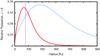 |
Fig. 2 Fractional population of level J = 6 from a model for a low mass-loss rate AGB star for 12CO (full red line) and 13CO (dashed blue line), with an isotopic ratio 12CO/13CO = 20. The vertical purple dashed line marks the point where critical density is reached for 12CO, calculated using the collisional coefficients between H2 and CO for a 300 K gas. 13CO reaches the critical density at a 5% greater distance. |
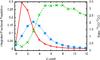 |
Fig. 3 Integrated relative 12CO and 13CO populations in a low mass-loss rate model envelope with an isotopic ratio 12CO/13CO = 20. 12CO is represented by the solid red line; 13CO, by the short-dashed blue line; and the ratio of the two, shown on the right-hand axis by the long-dashed green line. |
The point where the envelope reaches the critical density, below which collisional de-excitation is less probable than spontaneous de-excitation, is also shown in Fig. 2. Parameters such as the total H2 mass-loss rate, which indirectly set in our models by the 12CO abundance, and the stellar luminosity control the location of the point where the critical density is reached. The infrared stellar radiation field will have an impact on the excitation structure of the two molecules, mainly of 13CO, especially when the density is below critical. Therefore, uncertainties on the 12CO abundance, the stellar luminosity, and the infrared stellar radiation field will very likely lead to uncertainties on the determined isotopic ratio. Interferometric observations might be an important tool for determining the 12CO/13CO ratio more precisely, since those would show the region where emission originates for a given level of 12CO and 13CO, hence constraining the 12CO abundance and the importance of selective excitation of 13CO.
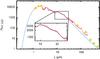 |
Fig. 4 Dust model (dashed blue line) compared to the ISO (red) and PACS and SPIRE (open yellow triangles) photometric observations and to near-IR photometric observations (filled yellow triangles). The fit to the silicate and amorphous aluminium oxide spectral features is shown in detail. The feature at 13 μm is not taken into account in our fit. |
4. Model for W Hya
4.1. Dust model
The model for the 12CO and 13CO emission from W Hya considers a dust component based on the parameters found by Justtanont et al. (2004), but fine-tuned to match our different approximation for calculating the extinction coefficient. This yielded slightly different abundances for each species and a smaller total dust mass-loss rate. We briefly discuss the dust model, stressing the points that are relevant for the CO emission analysis.
A total dust mass-loss rate of 2.8 × 10⁻¹⁰M⊙ yr-1 is needed to reproduce the SED with our dust model. Our best fit model contains 58% astronomical silicates, 34% amorphous aluminium oxide (Al2O3), and 8% magnesium-iron oxide (MgFeO). We prioritized fitting the region between 8 and 30 μm of the IR spectrum (see Fig. 4). However, we did not attempt to fit the 13 μm feature seen in the ISO spectrum of W Hya, since its origin is still a matter of debate. Candidate minerals that might account for this feature are crystalline aluminium oxides, either crystalline corundum (α-Al2O3) or spinel (MgAl2O4). One of these two species, at an abundance of less than 5%, might account for the observed 13 μm feature (see Posch et al. 1999; Zeidler et al. 2013, and references therein). We estimate an uncertainty on each of the derived dust abundances of 30%.
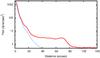 |
Fig. 5 Dust model (dashed blue) compared to the 70 μm PACS image (solid red line; Cox et al. 2012). |
The dust condensation radius found from the sublimation calculations is around 2.5 R⋆ for amorphous aluminium oxide (the species expected to condense first). This value is very similar to the 2 R⋆ inner radius of the shell of large transparent grains recently observed by Norris et al. (2012). The condensation radius found for the astronomical silicates is at 5 R⋆, approximately a factor of 5 lower than inferred by Zhao-Geisler et al. (2011) from interferometric observations. However, these authors calculated an average of several observations taken at different epochs, and this mean is dominated by the data taken during mid-IR maximum. The ISO spectrum we used was obtained shortly after the visual minimum phase. This may explain part of the discrepancy.
The dust model is compared to the ISO spectrum in Fig. 4 and to the recently published PACS 70 μm maps in Fig. 5. In the near infrared, W Hya’s spectrum is dominated by molecular absorption bands, which are not included in our models.
That the assumption of constant mass loss fits the 70 μm PACS maps up to about 20 arcsec (corresponding to 800 R⋆ for our adopted stellar parameters and distance) does not necessarily imply that the envelope is explained well by a constant dust mass-loss rate within that radius, since the contribution from the complex point-spread function is still important up to these distances. The good fit to the ISO spectrum between 10 μm and 30 μm, however, shows that the inner dust envelope is reproduced well by a constant mass-loss rate model. Interestingly, the 70 μm PACS image shows additional dust emission beyond 20 arcsec from the star, which is not expected on the basis of our model. Also, our model under-predicts the ISO spectrum from 30 μm onwards. It is possible that these two discrepancies between our model and the observations could be explained by the extra material around the star seen in the PACS images.
Furthermore, the point where the dust map shows extra emission, 800 R⋆, coincides with what is roughly expected for the CO dissociation radius from the predictions of Mamon et al. (1988) for a gas mass-loss rate of 1.5 × 10⁻⁷ M⊙ yr-1. Since much of the extra dust emission comes from outside of that radius, and we do not expect the extra supply of far-infrared photons produced by this dust to affect the CO excitation in a significant way, we will address the problem of the dust mass-loss history in a separate study. For the work carried out in this paper, it is important to stress that there seems to be an extra amount of material around the region where CO is typically expected to dissociate for a star such as W Hya. The origin of this extra material has not yet been identified and our model does not account for it.
4.2. Model for CO emission
Using GASTRoNOoM, we calculated a grid of models around the parameter values that are most often reported in the literature for W Hya. We used a two-step approach. First, the modelled line fluxes were compared to the SPIRE, PACS, HIFI, ISO, and ground-based observations using a reduced χ2 fit approach. Then, the line shapes were compared by eye to the normalized lines observed by HIFI and ground-based telescopes. Once we had found the region of parameter space with the lower reduced χ2 values and good line shapes fit, we refined the grid in this region in order to obtain our best grid model. The model parameters that are explored in our grid are presented in Table 2, together with the best fit values found by us.
Range of model parameters used for grid calculations.
4.2.1. Result from grid calculation
The best grid models have a terminal velocity of 7.5 km s-1, ϵ = 0.6 or 0.7, and a mass-loss rate of 1.5 × 10⁻⁷ M⊙ yr-1. The turbulent velocity may be determined from the steepness of the line wings, but could not be well constrained. Models with values of 1.0 km s-1 or higher all produce reasonable fits.
Figures 6–8 show the comparison of the best grid prediction with the observed integrated line fluxes, line shapes, and the PACS spectrum, respectively.
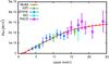 |
Fig. 6 Best grid model for the 12CO observed integrated line fluxes, when considering the dissociation radius as given by Mamon et al. (1988). Transition 12CO J = 16–15 observed by PACS and ISO is not used due to line blending (see Table 1). |
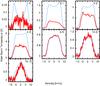 |
Fig. 7 Best grid model (in dashed blue) for the observed 12CO line shapes (in solid red), when considering the photodissociation radius as given by Mamon et al. (1988) compared to the observed line shapes. Observations were carried out by HIFI, APEX, SMT, and SEST (see Table 1). |
The overall fit of our best grid model to the line fluxes observed by SPIRE, PACS, HIFI, and ISO is quite good, and it does reproduce the broad trend of W Hya’s 12CO line emission. However, when we compare our model with the line shapes observed by HIFI and the ground-based measurements, we notice two things. First, as can be seen from Fig. 7, we over-predict the fluxes of the low-excitation 12CO lines, J = 4–3, J = 3–2, J = 2–1, and J = 1–0. Moreover, we predict the profiles to be double-peaked, while the observations do not show that. Since double-peaked line profiles are characteristic of an emission region that is spatially resolved by the beams of the telescopes, W Hya’s 12CO envelope seems to be smaller than what is predicted by our models. We discuss the problem of fitting the low-excitation lines in Sect. 4.2.5. Second, for the highest excitation line for which we have an observed line shape (12CO J = 16–15), our model not only over-predicts the flux observed by HIFI but also fails to match the width of the line profile. The observed triangular shape is characteristic of lines formed in the wind acceleration region (e.g. Bujarrabal et al. 1986). This indicates that either the wind acceleration is slower (equivalent to a higher β) or that the onset of the acceleration is more distant than the 2.5 R⋆ that is assumed in our grid and that corresponds to the condensation radius for amorphous Al2O3. This finding also implies that the velocity law may be more complex than the β-law Eq. (1). We return to this in Sect. 4.2.4.
4.2.2. 13CO abundance
Using our best grid model parameters, we calculated a small second grid of models, varying only the 12CO/13CO ratio and assuming an isotopologic ratio that is constant throughout the envelope.
The results are presented in Fig. 9. An isotopologic ratio of 20 fits the J = 10–9 and J = 9–8 transitions but somewhat over-predicts the J = 6–5 one. Transition J = 2–1 is predicted to be spatially resolved by SMT, though that is not supported by the observations.
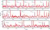 |
Fig. 8 Best grid model (in dashed blue) for the 12CO compared to the PACS spectrum (in solid red). Transition J = 23–22 of 12CO is blended with the water transition JKa,Kc = 41,4–30,3 at 113.54 μm line, and transition J = 22–21 is probably blended with both water transitions JKa,Kc = 93,7–84,4 and ν2 = 1, JKa,Kc = 43,2–50,5 at 118.41 μm and 118.98 μm, respectively. |
As discussed in Sect. 3, our models show that these two molecules have very different excitation structures throughout the envelope. In Fig. 10 we compare the excitation region of the upper levels of the 12CO J = 3–2, 12CO J = 4–3, 12CO J = 6–5, and 13CO J = 6–5 transitions for our best grid model. This comparison shows that the J = 6 level of 13CO has a similar excitation region to the J = 4 level for 12CO. Our probes of the outer wind are the line shapes and strengths of the 12CO J = 4–3 and lower excitation lines and the line strength of the 13CO J = 6–5 line. They all point in the direction of fewer 12CO and 13CO molecules in these levels in the outer wind than our model predicts.
4.2.3. The νLSR of W Hya
A value of 40.7 km s-1 is commonly found for the local standard of rest velocity, νLSR, of W Hya (e.g. Justtanont et al. 2005). However, there is still some uncertainty on this value, as determining it through different methods leads to slightly different results. For example, Uttenthaler et al. (2011) find a value of 40.5 km s-1, while Etoka et al. (2001) suggest 40.6 ± 0.4.
The value of νLSR that best fits our data is 40.4 km s-1. By shifting the modeled lines by this amount, the model fits the lines of 12CO and transition J = 6–5 of 13CO well. For the J = 10–9 and J = 9–8 transitions of 13CO, a νLSR of 39.6 km s-1 seems more appropriate. These two lines are also narrower than our model predicts. This difference points to an asymmetry in the wind expansion, the blue shifted-wing being accelerated faster than the red-wing one. A direction-dependent acceleration from the two higher excitation lines of 13CO is not, however, conclusive at this point.
4.2.4. Fitting the high-excitation lines: velocity profile
A value of 1.5 for the exponent of the β-type velocity profile over-predicts the width of 12CO J = 16–15 observed by HIFI. To reproduce the narrow line profile observed for this high excitation transition, we have to increase β to about 5.0. This corresponds to a very slowly accelerating wind. Increasing β affects not only the line shapes but also the line fluxes. To maintain the fit to the observed fluxes, we have to decrease the mass-loss rate by about 10% to 1.3 × 10⁻⁷M⊙ yr-1. With this change, the low-excitation lines also become roughly 10% weaker. This helps, but does not solve the problem of fitting these lines.
The line shapes of transitions J = 10–9 and J = 6–5 of 12CO and J = 10–9 and J = 9–8 of 13CO (see Figs. 11 and 13) are strongly affected by these changes. In Fig. 11 we show the comparison of our best grid model with the model with β = 5.0 and lower mass-loss rate. As can be seen, the line shape of transition 12CO J = 16–15 is much better fitted by the higher value of β. For transition 12CO J = 10–9, that is also the case for the red wing but not for the blue wing. For transition 12CO J = 6–5, the model with β = 5.0 predicts too narrow a line, while the model with β = 1.5 matches the red wing but slightly over-predicts the emission seen in the blue wing.
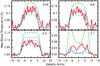 |
Fig. 9 Model calculations for different 12CO/13CO ratios compared to the observed 13CO lines adopting the dissociation radius by Mamon et al. (1988). The solid red line represents the observations. The long-dashed green, short-dashed blue, dotted purple, and dot-dashed light blue lines are for intrinsic isotope ratios 10, 15, 20, and 30, respectively. Transitions J = 10–9 and 9–8 have been smoothed for a better visualization. |
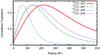 |
Fig. 10 Relative population distribution of different levels of 12CO and 13CO for our best grid model. |
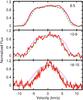 |
Fig. 11 Normalized predicted line shapes for different values of the velocity law exponent compared to the normalized observed line shapes of the 12CO transitions observed by HIFI. The observations are shown by the solid red line, the dashed green line represents a model with β = 5.0, and the dotted purple line a model with β = 1.5. |
Another possibility for decreasing the width of the high excitation lines is to set the starting point of the acceleration of the wind, r° in Eq. (1), further out. For those of our models discussed so far, the starting point of the acceleration is set at the condensation radius of the first dust species to form (amorphous Al2O3), which is at 2.5 R⋆. We need to set r° to 8 R⋆ to get a good fit to the line profile of transition 12CO J = 16–15. As when β is changed, we need to decrease the mass-loss rate by approximately 10% to compensate for the higher density in the inner wind.
Increasing the value of r° has a similar impact to increasing the value of β and, therefore, models with different combinations of these parameters will be able to reproduce the observed line shapes. That the wind has a slower start than expected, either because the gas acceleration starts further out or a very gradual acceleration is consistent with previous interferometric measurements of SiO, H2O, and OH maser emission (Szymczak et al. 1998) and of SiO pure rotational emission (Lucas et al. 1992).
From the final values found for the dust (2.8 × 10⁻¹⁰M⊙ yr-1) and gas (1.3 × 10⁻⁷M⊙ yr-1) mass-loss rate, we derive a value for the dust-to-gas ratio of 2 × 10⁻³. Considering an uncertainty of 50% for both the derived dust and the gas mass-loss rates, we estimate the uncertainty on this value to be approximately 70%.
4.2.5. Fitting the low-excitation lines
We now investigate why, within the parameter space region spanned by our grid calculation, we cannot simultaneously fit the line fluxes of the intermediate and high excitation lines (Jup ≥ 6) and the line fluxes and shapes of the low excitation lines (Jup ≤ 4).
One possible cause could be a variable mass loss. In this case, the low excitation transitions would be tracing gas that was ejected when the mass-loss rate was lower than what it is presently, which is traced by the higher excitation lines. This would be in strong contrast, however, to what we expect from the spatial distribution of the dust, since the PACS 70 μm image shows that there is more dust emission at distances greater than the 20 arcsec (≈800 R⋆) that our dust model can account for. To reconcile this, we would have to invoke not only a change in mass-loss rate but also quite an arbitrary and difficult-to-justify change in the dust-to-gas ratio. Therefore, we argue that a mass-loss rate discontinuity is not a likely explanation for the problem of fitting the low excitation lines in our model of W Hya.
Another possibility would be to consider a broken temperature law with a different exponent for the outer region where the low-excitation lines are formed. We can either increase the exponent given in Eq. (2) to obtain lower temperatures in the outer regions or decrease the exponent to have higher temperatures in the outer regions. Changing the gas temperature does not necessarily have a big impact on the 12CO level populations because the radiation field also plays an important role in the excitation.
We calculated models with both higher (0.9) and lower (0.4) values of ϵ for the outer regions assuming two different breaking points for the temperature power law, either at 80 or 150 R⋆. The breaking points were chosen based on the excitation region of the low-excitation lines, since at 150 R⋆ the population of level J = 4 of 12CO peaks. The models with a breaking point at 80 R⋆ represents an intermediate step between introducing a breakpoint that will only affect the low-excitation lines and changing the exponent of the temperature law in the entire wind. We find that the strength of the low-excitation lines relative to each other changes but that the overall fit does not improve, since most of the lines are still over-predicted. This suggests that we need a lower CO abundance in the outer envelope.
Following Justtanont et al. (2005), another option for tacklng the problem is to vary the parameter that controls the point from which dissociation of CO happens, r1/2. We calculated new models considering values r1/2 = 0.2, 0.3, 0.4, 0.5, and 0.8 . This corresponds to a stronger dissociation than a value of unity, which corresponds to the prediction of Mamon et al. (1988), and, therefore, a smaller CO radius. For  , the CO abundance has decreased by half at ~860 stellar radii. This is at about the region where the PACS images show that there is more dust emission than predicted by our dust model. By decreasing r1/2 to 0.4 , which corresponds to CO reaching half of the initial abundance around 350 stellar radii, being 40% of the size predicted by (Mamon et al. 1988), we could fit the shape of transitions 12CO J = 4–3, 12CO J = 3–2, and 12CO J = 2–1 and the total flux of transitions 12CO J = 3–2 and 12CO J = 2–1. The strength of transition 12CO J = 4–3 is still over-predicted by 60% by this new model, and the number of CO molecules in the J = 1 level becomes so small that the 12CO J = 1–0 transition is predicted to be too weak to observe.
Because the PACS image shows an unexpectedly strong dust emission at the radii where we expect the J = 1–0 line of 12CO to be excited (the J = 1 level population reaches its maximum at 1000 R⋆ in the absence of photo-dissociation), we do not attempt to model this emission further in the context of our model assumptions.
The fit using r1/2 = 0.4 does not affect the flux of J = 8–7 and higher excitation lines, because those are formed deep inside the envelope. The model with smaller CO radius and β = 5.0 is compared to the observed 12CO line shapes in Fig. 12.
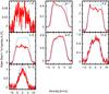 |
Fig. 12 Model with r1/2 = 0.4, β = 5.0, and Ṁ= 1.3 × 10⁻⁷ M⊙ yr-1 for 12CO (in dashed blue) compared to observed line shapes (in solid red). Observations were carried out by HIFI, APEX, SMT, and SEST (see Table 1). |
In Fig. 13 we show models for the 13CO transitions, considering the smaller dissociation radius and β = 5.0. The 13CO J = 10–9, 13CO J = 9–8, and 13CO J = 6–5 lines are now more consistently fitted by an isotopic ratio between 15 and 20. In Sect. 5 we discuss the uncertainty on the determined isotopic ratio. The predicted 13CO J = 2–1 emission is so weak that it should not be measurable, similar to 12CO J = 1–0. Since the population of level J = 2 of 13CO peaks even further out than J = 1 of 12CO, we also refrain from explaining the emission in this line in the context of our current model.
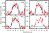 |
Fig. 13 Models with r1/2 = 0.4, β = 5.0, and Ṁ= 1.3 × 10⁻⁷M⊙ yr-1 compared to the 13CO observed lines. The solid red line represents the observations. The long-dashed green, short-dashed blue, dotted pink, and dot-dashed light blue lines represent models with 12C/13C = 10, 15, 20, and 30, respectively. A value of 18 for the 12C/13C ratio reproduces the data best. |
5. Discussion
5.1. The outer CO envelope
The modelling of W Hya suggests a wind structure that is atypical of oxygen-rich AGB sources, both in terms of the behaviour of the CO gas and of the dust, particularly so near the CO photodissociation zone. Using maps of 12CO J = 2–1 and 12CO J = 1–0 for other sources, Castro-Carrizo et al. (2010) show that the location of this zone matches, or is larger than, the photodissociation radius predicted by Mamon et al. (1988). The strengths and shapes of low-excitation lines (Jup ≤ 4) in W Hya, however, clearly indicate that the size of the CO envelope is significantly smaller than predicted by Mamon et al. (1988). That the situation is complex may be discerned from the 12CO J = 1–0 and 13CO J = 2–1 pure rotational lines. Weak emission is observed for these lines, but no emission is predicted when we adopt r1/2 = 0.4 . These lines are, however, mainly excited in the outer parts of the CO envelope (r ≳ 600 R⋆, or 15″ for the adopted stellar parameters and distance), a region where the PACS images show that the envelope of W Hya is not predicted well by our constant mass-loss rate model.
5.2. The 12CO/13CO ratio
For the first time, we have multiple isotopic transitions in 12CO and 13CO available to constrain the 12CO/13CO isotopologic ratio. Three of the four lines for which we have data for the 13CO isotopologue, i.e. J = 10–9, 9–8, and 6–5, point to an intrinsic 12CO/13CO ratio of 18. For comparison, the line ratios between the two isotopologues observed by HIFI are around 8 and 8.7 for transitions J = 10–9 and J = 6–5, respectively. The only previous attempt to constrain the intrinsic ratio is by Milam et al. (2009), who found a value of 35 using the J = 2–1 of 13CO transition. We could not use this particular transition, since it is poorly reproduced by our model. We note that Milam et al. considered a mass loss that is an order of magnitude greater than was found by us and Justtanont et al. (2005), and a three times lower 12CO abundance. They also assumed W Hya to be at a distance of 115 pc, which implies a twice higher luminosity than we have adopted. Given the intricacies in forming the 12CO and 13CO lines, especially in the case of the outer envelope of W Hya, it is hard to assess the meaning of the factor-of-two difference in the intrinsic 12C/13C. We therefore discuss the uncertainties in this ratio in more detail. This discussion is also important in view of a comparison with theoretical predictions, this ratio being a very useful tool for constraining AGB evolution models.
5.2.1. The uncertainty of the determined 12CO/13CO ratio
In order to quantify the robustness of the derived 12CO/13CO ratio, we carried out a test in which we vary parameters that so far were held fixed in our model grid and studied the effect.
First, we investigate the impact of varying the assumed 12CO abundance relative to H (standard at 2.0 × 10⁻⁴) and the stellar luminosity considered (5400 L⊙). We calculated models in which we changed each of these parameters, but only one at a time, by a factor of two – both toward higher and lower values. When these parameters are varied, the 12CO line fluxes and shapes also change. We scaled the mass-loss rate in order to fit the line flux observed by SPIRE, since the 12CO lines observed by this instrument are excited in the same region as 13CO transitions used to determine the isotopic ratio. We did not attempt a fine-tuning to match the strengths and shapes of the profiles. The factor-of-two changes in each of the two parameters affect the line fluxes of 13CO by typically 20 to 25 per cent and at most 30 per cent.
Second, we studied the effect of changes in the input stellar spectrum. As pointed out in Sect. 3, the stellar flux in the near infrared may have an important effect on the CO line strengths as photons of these wavelengths can efficiently pump molecules to higher rotational levels. In our models, the spectral emission of W Hya is approximated by a black body of 2500 K. However, the stellar spectrum is much more complex, and its intensity changes considerably even for small differences in wavelength. Specifically, molecules in the stellar atmosphere can absorb photons, thereby reducing the amount available for exciting 12CO and 13CO further out in the envelope. Figure 4 indicates that the molecular absorption at 4.7 μm is less than a factor of two. We assume a factor-of-two decrease in the stellar flux in the 4.7 μm region to assess the impact of the near-IR flux on the modelled lines. The change in the integrated line flux of 12CO lines is only about five per cent. The 13CO lines respond more strongly, varying by typically 25%.
The combined impact of these three sources of uncertainties on the derived isotopic ratio would be ~40% in this simple approach. Also accounting for uncertainties due to the flux calibration and noise (which are about 25% uncertain) and the actual model fitting (25% uncertain), we conclude that the intrinsic isotopic ratio determined here is uncertain by 50% to 60%. This implies that W Hya has a 12CO/13CO ratio of 18 ± 10. Better signal-to-noise observations of, particularly, 13CO, in combination with spatial maps of both 12CO and 13CO lines, are required to constrain this value better.
5.2.2. Connecting the 12C/13C ratio to stellar evolution
From evolutionary model calculations, the surface 12C/13C ratio is expected to change in dredge-up events. It is found to decrease by a factor of a few after the first dredge-up, taking place during the ascent on the red giant branch (RGB) and reaching a value of typically 20 for stars more massive than 2 M⊙. For stars with masses lower than 2 M⊙, it is found to increase with decreasing mass, reaching about 30 at 0.8 M⊙. In stars that experience the second dredge-up (M⋆ ≳ 4.5 M⊙), this ratio is found to decrease further by a few tens of per cent during the ascent on the AGB (Busso et al. 1999; Karakas 2011). Stars with masses higher than 1.5 M⊙ experience the third dredge-up, a continuous process that occurs during the thermally pulsing AGB phase. Evolutionary models show that this ratio is steadily increasing thanks to the surface enrichment of 12C or is not changing significantly if the star is massive enough, M⋆ ≳ 4.0 M⊙, for hot bottom burning to operate.
Recent calculations include extra-mixing processes to explain the low values of the 12C/13C ratio observed in low mass RGB stars (Tsuji 2007; Smiljanic et al. 2009; Mikolaitis et al. 2012). Extra-mixing processes are thought to occur also during the AGB phase (Busso et al. 2010), but its causes and consequences are more uncertain. Models that include extra mixing in the RGB predict lower isotopic ratios (~10) for low mass stars (~1 M⊙).
When compared to model predictions, a value of 18 for the 12C/13C ratio would be consistent with W Hya having an isotopic ratio that reflects the value set by the first dredge-up (Boothroyd & Sackmann 1999; Charbonnel & Lagarde 2010) for star with masses higher than about 2 M⊙. If W Hya’s mass lies between 1.5 M⊙ and 4.0 M⊙, the value found by us further suggests that the star has experienced few or none of these third dredge-up events.
Our intrinsic isotopic ratio, however, is not very constraining, since it agrees within the uncertainties with three very different scenarios for W Hya’s evolutionary stage: first, having a low value of this ratio (~8), hence having suffered extra mixing in the first dredge-up, characteristic of low mass stars; second, having a ratio of indeed 18, which implies a higher mass; or, third, having a higher ratio (~28) and being on its way to becoming a carbon star. Decreasing the error bars by a factor of three or four would allow one to draw stronger conclusions on this matter. Such accuracy may be achieved with the Atacama Large Millimeter/submillimeter Array.
5.3. The wind acceleration
The wind acceleration in W Hya is quite slow. The highest excitation line for which we have an observed line shape, 12CO J = 16–15, has an excitation of its upper level that peaks at eight stellar radii, decreasing to one-fifth of this peak value at 30 R⋆. The triangular shape and the width of this profile indicate that it is formed in the accelerating part of the flow. The 12CO J = 10–9 line is still explained well by a β = 5.0 model, but the region where this line is excited seems to be where the wind starts to be accelerated faster than our model with β = 5.0. Interestingly, this effect is noted mainly in the blue-shifted part of the flow. The population of level J = 10 of 12CO reaches a maximum at 25 R⋆, decreasing to one-fifth of this peak value at 70 R⋆. This shows that the wind approaches the terminal velocity indeed much later than expected, somewhere around 50 stellar radii. Furthermore, transition J = 6–5 of 12CO is formed in a region where the wind has already reached maximum expansion velocity, contrary to what a model with β = 5.0 predicts. This indicates that, although the wind has a slow start until 5.5–6.0 km s-1, the last injection of momentum happens quite fast. Other authors have also concluded that the wind of W Hya is accelerated slower than expected (Lucas et al. 1992; Szymczak et al. 1998), in agreement with our results.
The shapes of 13CO J = 10–9 and J = 9–8 lines are also asymmetric, as is that of 12CO J = 10–9 line. The reason for this is not clear but may be connected to large scale inhomogeneities that damp out, or smooth out, at large distances. A direction-dependent acceleration law, for example, or direction-dependent excitation structures of the higher levels of these two transitions might be the reason we see this asymmetry. The higher optical depth in the 12CO lines might be able to make this feature less pronounced in the J = 10–9 of this isotopologue. We note that these two 13CO lines do not have a high signal-to-noise ratio, therefore, no firm conclusion can be drawn based on this apparent asymmetry.
6. Summary
We have constrained the wind structure of W Hya using an unprecedented number of 12CO and 13CO emission lines. We were especially interested in understanding the excitation of 12CO and 13CO for this source. The envelope structure derived in this study will enable analysis of other molecular abundances in the outflow, such as ortho- and para-water and its isotopologues, SiO and its isotopologues, SO, SO2, and even carbon-based molecules such as HCN. Specifically, we may thus obtain excitation conditions of these molecules and the heating and cooling rates – mainly thanks to water transitions – associated to it. These species too will add to our understanding of the physical and chemical processes in the wind.
The main conclusions obtained from modelling 12CO and 13CO are
-
The model that best fits the data has a mass-loss rateof 1.3 × 10⁻⁷ M⊙ yr-1, an expansion velocityof 7.5 km s-1, atemperature power-law exponent of 0.65, a COdissociation radius 2.5 timessmaller than what is predicted by theory, and an exponent ofthe β-type velocity law of 5.0. Wenote that the wind has a slow start that is better reproduced by a highvalue of this exponent, but that the envelope reaches its finalexpansion velocity sooner than such a model would predict.
-
The smaller outer CO radius is supported mainly by the line strengths of the low-J lines. Introducing a broken temperature law does not fix this problem, and a varying mass-loss rate, lower in the outer envelope, seems to contradict what is seen in the PACS dust maps.
-
By comparing our constant mass-loss rate dust model with recently published PACS images of W Hya, we note that our dust model does not reproduce the observations beyond 20″, corresponding to 800 R⋆ for the adopted parameters and distance. This extra emission may originate in material expelled in a phase of higher mass loss or be the result of a build up of material from interaction with previously ejected gas or interstellar medium gas.
-
We derive a 12CO to 13CO isotopic ratio of 18 ± 10. The accuracy is not sufficient to draw firm conclusions on the evolutionary stage or main-sequence mass of W Hya, but a ratio of 20 would be expected for an AGB star with mass higher than 2 M⊙ that did not experience 12C enrichment due to the third dredge-up phase. Spatially resolved observations may help constrain the 12CO abundance and the 13CO excitation region and allow for a more precise estimate of this ratio.
Acknowledgments
HIFI has been designed and built by a consortium of institutes and university departments from across Europe, Canada, and the United States under the leadership of SRON Netherlands Institute for Space Research, Groningen, The Netherlands, and with major contributions from Germany, France, and the USA. Consortium members are Canada: CSA, U. Waterloo; France: CESR, LAB, LERMA, IRAM; Germany: KOSMA, MPIfR, MPS; Ireland, NUI Maynooth; Italy: ASI, IFSI-INAF, Osservatorio Astrofisico di Arcetri-INAF; Netherlands: SRON, TUD; Poland: CAMK, CBK; Spain: Observatorio Astronómico Nacional (IGN), Centro de Astrobiología (CSIC-INTA). Sweden: Chalmers University of Technology MC2, RSS & GARD, Onsala Space Observatory, Swedish National Space Board, Stockholm University SStockholm Observatory; Switzerland: ETH Zurich, FHNW; USA: Caltech, JPL, NHSC. PACS has been developed by a consortium of institutes led by MPE (Germany) and including UVIE (Austria); KUL, CSL, IMEC (Belgium); CEA, OAMP (France); MPIA (Germany); IFSI, OAP/AOT, OAA/CAISMI, LENS, SISSA (Italy); IAC (Spain). This development has been supported by the funding agencies BMVIT (Austria), ESA-PRODEX (Belgium), CEA/CNES (France), DLR (Germany), ASI (Italy), and CICYT/MCYT (Spain). SPIRE has been developed by a consortium of institutes led by Cardiff Univ. (UK) and including Univ. Lethbridge (Canada); NAOC (China); CEA, LAM (France); IFSI, Univ. Padua (Italy); IAC (Spain); Stockholm Observatory (Sweden); Imperial College London, RAL, UCL-MSSL, UKATC, Univ. Sussex (UK); Caltech, JPL, NHSC, Univ. Colorado (USA). This development has been supported by national funding agencies: CSA (Canada); NAOC (China); CEA, CNES, CNRS (France); ASI (Italy); MCINN (Spain); SNSB (Sweden); STFC (UK); and NASA (USA). T.Kh. gratefully acknowledges support from NWO grant 614.000.903. R.Sz. and M.Sch. acknowledge support from NCN grant N 203 581040. This work has been partially supported by the Spanish MICINN, programme CONSOLIDER INGENIO 2010, grant “ASTROMOL” (CSD2009-00038). J.B., P.R., B.v.B. acknowledge support from the Belgian Science Policy Office through the ESA PRODEX programme. F.K. is supported by the FWF project P23586 and the ffg ASAP project HIL.
References
- Barlow, M. J., Nguyen-Q-Rieu, Truong-Bach, et al. 1996, A&A, 315, L241 [NASA ADS] [Google Scholar]
- Begemann, B., Dorschner, J., Henning, T., et al. 1997, ApJ, 476, 199 [NASA ADS] [CrossRef] [Google Scholar]
- Bohren, C. F., & Huffman, D. R. 1998, Absorption and Scattering of Light by Small Particles (Wiley) [Google Scholar]
- Boothroyd, A. I., & Sackmann, I.-J. 1999, ApJ, 510, 232 [Google Scholar]
- Bujarrabal, V., Planesas, P., Martin-Pintado, J., Gomez-Gonzalez, J., & del Romero, A. 1986, A&A, 162, 157 [NASA ADS] [Google Scholar]
- Busso, M., Gallino, R., & Wasserburg, G. J. 1999, ARA&A, 37, 239 [NASA ADS] [CrossRef] [Google Scholar]
- Busso, M., Palmerini, S., Maiorca, E., et al. 2010, ApJ, 717, L47 [NASA ADS] [CrossRef] [Google Scholar]
- Castro-Carrizo, A., Quintana-Lacaci, G., Neri, R., et al. 2010, A&A, 523, A59 [NASA ADS] [CrossRef] [EDP Sciences] [Google Scholar]
- Charbonnel, C., & Lagarde, N. 2010, A&A, 522, A10 [NASA ADS] [CrossRef] [EDP Sciences] [MathSciNet] [PubMed] [Google Scholar]
- Cox, N. L. J., Kerschbaum, F., van Marle, A.-J., et al. 2012, A&A, 537, A35 [NASA ADS] [CrossRef] [EDP Sciences] [Google Scholar]
- Cristallo, S., Piersanti, L., Straniero, O., et al. 2011, ApJS, 197, 17 [NASA ADS] [CrossRef] [Google Scholar]
- De Beck, E., Decin, L., de Koter, A., et al. 2010, A&A, 523, A18 [NASA ADS] [CrossRef] [EDP Sciences] [Google Scholar]
- de Graauw, T., Helmich, F. P., Phillips, T. G., et al. 2010, A&A, 518, L6 [NASA ADS] [CrossRef] [EDP Sciences] [Google Scholar]
- Decin, L., Hony, S., de Koter, A., et al. 2006, A&A, 456, 549 [NASA ADS] [CrossRef] [EDP Sciences] [Google Scholar]
- Decin, L., De Beck, E., Brünken, S., et al. 2010, A&A, 516, A69 [NASA ADS] [CrossRef] [EDP Sciences] [Google Scholar]
- Etoka, S., Błaszkiewicz, L., Szymczak, M., & Le Squeren, A. M. 2001, A&A, 378, 522 [NASA ADS] [CrossRef] [EDP Sciences] [Google Scholar]
- Glass, I. S., & van Leeuwen, F. 2007, MNRAS, 378, 1543 [NASA ADS] [CrossRef] [Google Scholar]
- Griffin, M. J., Abergel, A., Abreu, A., et al. 2010, A&A, 518, L3 [Google Scholar]
- Groenewegen, M. A. T., Waelkens, C., Barlow, M. J., et al. 2011, A&A, 526, A162 [NASA ADS] [CrossRef] [EDP Sciences] [Google Scholar]
- Habing, H. J., & Olofsson, H. 2003, Asymptotic Giant Branch Stars, Astron. Astrophys. Lib. (New York, Berlin: Springer) [Google Scholar]
- Harwit, M., & Bergin, E. A. 2002, ApJ, 565, L105 [NASA ADS] [CrossRef] [Google Scholar]
- Hawkins, G. W. 1990, A&A, 229, L5 [Google Scholar]
- Henning, T., Begemann, B., Mutschke, H., & Dorschner, J. 1995, A&AS, 112, 143 [NASA ADS] [Google Scholar]
- Iben, Jr., I. 1975, ApJ, 196, 525 [NASA ADS] [CrossRef] [Google Scholar]
- Iben, Jr., I., & Renzini, A. 1983, ARA&A, 21, 271 [NASA ADS] [CrossRef] [Google Scholar]
- Justtanont, K., & Tielens, A. G. G. M. 1992, ApJ, 389, 400 [CrossRef] [Google Scholar]
- Justtanont, K., de Jong, T., Tielens, A. G. G. M., Feuchtgruber, H., & Waters, L. B. F. M. 2004, A&A, 417, 625 [NASA ADS] [CrossRef] [EDP Sciences] [Google Scholar]
- Justtanont, K., Bergman, P., Larsson, B., et al. 2005, A&A, 439, 627 [NASA ADS] [CrossRef] [EDP Sciences] [Google Scholar]
- Justtanont, K., Khouri, T., Maercker, M., et al. 2012, A&A, 537, A144 [NASA ADS] [CrossRef] [EDP Sciences] [Google Scholar]
- Kama, M., Min, M., & Dominik, C. 2009, A&A, 506, 1199 [NASA ADS] [CrossRef] [EDP Sciences] [Google Scholar]
- Karakas, A. I. 2010, MNRAS, 403, 1413 [NASA ADS] [CrossRef] [Google Scholar]
- Karakas, A. I. 2011, in Why Galaxies Care about AGB Stars II: Shining Examples and Common Inhabitants, eds. F. Kerschbaum, T. Lebzelter, & R. F. Wing, ASP Conf. Ser., 445, 3 [Google Scholar]
- Kessler, M. F., Steinz, J. A., Anderegg, M. E., et al. 1996, A&A, 315, L27 [NASA ADS] [Google Scholar]
- Knapp, G. R., Pourbaix, D., Platais, I., & Jorissen, A. 2003, A&A, 403, 993 [NASA ADS] [CrossRef] [EDP Sciences] [Google Scholar]
- Lombaert, R., Decin, L., de Koter, A., et al. 2013, A&A, 554, A142 [NASA ADS] [CrossRef] [EDP Sciences] [Google Scholar]
- Lucas, R., Bujarrabal, V., Guilloteau, S., et al. 1992, A&A, 262, 491 [NASA ADS] [Google Scholar]
- Maercker, M., Schöier, F. L., Olofsson, H., Bergman, P., & Ramstedt, S. 2008, A&A, 479, 779 [NASA ADS] [CrossRef] [EDP Sciences] [Google Scholar]
- Maercker, M., Schöier, F. L., Olofsson, H., et al. 2009, A&A, 494, 243 [NASA ADS] [CrossRef] [EDP Sciences] [Google Scholar]
- Mamon, G. A., Glassgold, A. E., & Huggins, P. J. 1988, ApJ, 328, 797 [NASA ADS] [CrossRef] [Google Scholar]
- Mathis, J. S., Rumpl, W., & Nordsieck, K. H. 1977, ApJ, 217, 425 [NASA ADS] [CrossRef] [Google Scholar]
- Mikolaitis, Š., Tautvaišienė, G., Gratton, R., Bragaglia, A., & Carretta, E. 2012, A&A, 541, A137 [NASA ADS] [CrossRef] [EDP Sciences] [Google Scholar]
- Milam, S. N., Woolf, N. J., & Ziurys, L. M. 2009, ApJ, 690, 837 [NASA ADS] [CrossRef] [Google Scholar]
- Min, M., Hovenier, J. W., & de Koter, A. 2003, A&A, 404, 35 [NASA ADS] [CrossRef] [EDP Sciences] [Google Scholar]
- Min, M., Dullemond, C. P., Dominik, C., de Koter, A., & Hovenier, J. W. 2009, A&A, 497, 155 [NASA ADS] [CrossRef] [EDP Sciences] [Google Scholar]
- Morris, M. 1980, ApJ, 236, 823 [NASA ADS] [CrossRef] [Google Scholar]
- Naylor, D. A., & Tahic, M. K. 2007, J. Opt. Soc. Am. A, 24, 3644 [NASA ADS] [CrossRef] [Google Scholar]
- Neufeld, D. A., Chen, W., Melnick, G. J., et al. 1996, A&A, 315, L237 [NASA ADS] [Google Scholar]
- Norris, B. R. M., Tuthill, P. G., Ireland, M. J., et al. 2012, Nature, 484, 220 [NASA ADS] [CrossRef] [PubMed] [Google Scholar]
- Perryman, M. A. C., & ESA 1997, The HIPPARCOS and TYCHO catalogues. Astrometric and photometric star catalogues derived from the ESA HIPPARCOS Space Astrometry Mission, ESA SP, 1200 [Google Scholar]
- Pilbratt, G. L., Riedinger, J. R., Passvogel, T., et al. 2010, A&A, 518, L1 [CrossRef] [EDP Sciences] [Google Scholar]
- Poglitsch, A., Waelkens, C., Geis, N., et al. 2010, A&A, 518, L2 [NASA ADS] [CrossRef] [EDP Sciences] [Google Scholar]
- Posch, T., Kerschbaum, F., Mutschke, H., et al. 1999, A&A, 352, 609 [NASA ADS] [Google Scholar]
- Schöier, F. L., & Olofsson, H. 2000, A&A, 359, 586 [NASA ADS] [Google Scholar]
- Smiljanic, R., Gauderon, R., North, P., et al. 2009, A&A, 502, 267 [NASA ADS] [CrossRef] [EDP Sciences] [Google Scholar]
- Szymczak, M., Cohen, R. J., & Richards, A. M. S. 1998, MNRAS, 297, 1151 [NASA ADS] [CrossRef] [Google Scholar]
- Tsuji, T. 2007, in IAU Symp., 239, eds. F. Kupka, I. Roxburgh, & K. L. Chan, 307 [Google Scholar]
- Uttenthaler, S., van Stiphout, K., Voet, K., et al. 2011, A&A, 531, A88 [NASA ADS] [CrossRef] [EDP Sciences] [Google Scholar]
- Ventura, P., & Marigo, P. 2009, MNRAS, 399, L54 [NASA ADS] [CrossRef] [Google Scholar]
- Vlemmings, W. H. T., Humphreys, E. M. L., & Franco-Hernández, R. 2011, ApJ, 728, 149 [NASA ADS] [CrossRef] [Google Scholar]
- Wing, R. F. 1971, PASP, 83, 301 [NASA ADS] [CrossRef] [Google Scholar]
- Zeidler, S., Posch, T., & Mutschke, H. 2013, A&A, 553, A81 [NASA ADS] [CrossRef] [EDP Sciences] [Google Scholar]
- Zhao-Geisler, R., Quirrenbach, A., Köhler, R., Lopez, B., & Leinert, C. 2011, A&A, 530, A120 [NASA ADS] [CrossRef] [EDP Sciences] [Google Scholar]
- Zubko, V., & Elitzur, M. 2000, ApJ, 544, L137 [NASA ADS] [CrossRef] [Google Scholar]
All Tables
All Figures
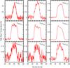 |
Fig. 1 Observed line profiles of 12CO and 13CO. The data is from HIFI, APEX and SMT (see Table 1). |
| In the text | |
|
Fig. 2 Fractional population of level J = 6 from a model for a low mass-loss rate AGB star for 12CO (full red line) and 13CO (dashed blue line), with an isotopic ratio 12CO/13CO = 20. The vertical purple dashed line marks the point where critical density is reached for 12CO, calculated using the collisional coefficients between H2 and CO for a 300 K gas. 13CO reaches the critical density at a 5% greater distance. |
| In the text | |
|
Fig. 3 Integrated relative 12CO and 13CO populations in a low mass-loss rate model envelope with an isotopic ratio 12CO/13CO = 20. 12CO is represented by the solid red line; 13CO, by the short-dashed blue line; and the ratio of the two, shown on the right-hand axis by the long-dashed green line. |
| In the text | |
|
Fig. 4 Dust model (dashed blue line) compared to the ISO (red) and PACS and SPIRE (open yellow triangles) photometric observations and to near-IR photometric observations (filled yellow triangles). The fit to the silicate and amorphous aluminium oxide spectral features is shown in detail. The feature at 13 μm is not taken into account in our fit. |
| In the text | |
|
Fig. 5 Dust model (dashed blue) compared to the 70 μm PACS image (solid red line; Cox et al. 2012). |
| In the text | |
|
Fig. 6 Best grid model for the 12CO observed integrated line fluxes, when considering the dissociation radius as given by Mamon et al. (1988). Transition 12CO J = 16–15 observed by PACS and ISO is not used due to line blending (see Table 1). |
| In the text | |
|
Fig. 7 Best grid model (in dashed blue) for the observed 12CO line shapes (in solid red), when considering the photodissociation radius as given by Mamon et al. (1988) compared to the observed line shapes. Observations were carried out by HIFI, APEX, SMT, and SEST (see Table 1). |
| In the text | |
|
Fig. 8 Best grid model (in dashed blue) for the 12CO compared to the PACS spectrum (in solid red). Transition J = 23–22 of 12CO is blended with the water transition JKa,Kc = 41,4–30,3 at 113.54 μm line, and transition J = 22–21 is probably blended with both water transitions JKa,Kc = 93,7–84,4 and ν2 = 1, JKa,Kc = 43,2–50,5 at 118.41 μm and 118.98 μm, respectively. |
| In the text | |
|
Fig. 9 Model calculations for different 12CO/13CO ratios compared to the observed 13CO lines adopting the dissociation radius by Mamon et al. (1988). The solid red line represents the observations. The long-dashed green, short-dashed blue, dotted purple, and dot-dashed light blue lines are for intrinsic isotope ratios 10, 15, 20, and 30, respectively. Transitions J = 10–9 and 9–8 have been smoothed for a better visualization. |
| In the text | |
|
Fig. 10 Relative population distribution of different levels of 12CO and 13CO for our best grid model. |
| In the text | |
|
Fig. 11 Normalized predicted line shapes for different values of the velocity law exponent compared to the normalized observed line shapes of the 12CO transitions observed by HIFI. The observations are shown by the solid red line, the dashed green line represents a model with β = 5.0, and the dotted purple line a model with β = 1.5. |
| In the text | |
|
Fig. 12 Model with r1/2 = 0.4, β = 5.0, and Ṁ= 1.3 × 10⁻⁷ M⊙ yr-1 for 12CO (in dashed blue) compared to observed line shapes (in solid red). Observations were carried out by HIFI, APEX, SMT, and SEST (see Table 1). |
| In the text | |
|
Fig. 13 Models with r1/2 = 0.4, β = 5.0, and Ṁ= 1.3 × 10⁻⁷M⊙ yr-1 compared to the 13CO observed lines. The solid red line represents the observations. The long-dashed green, short-dashed blue, dotted pink, and dot-dashed light blue lines represent models with 12C/13C = 10, 15, 20, and 30, respectively. A value of 18 for the 12C/13C ratio reproduces the data best. |
| In the text | |
Current usage metrics show cumulative count of Article Views (full-text article views including HTML views, PDF and ePub downloads, according to the available data) and Abstracts Views on Vision4Press platform.
Data correspond to usage on the plateform after 2015. The current usage metrics is available 48-96 hours after online publication and is updated daily on week days.
Initial download of the metrics may take a while.