| Issue |
A&A
Volume 561, January 2014
|
|
|---|---|---|
| Article Number | A98 | |
| Number of page(s) | 9 | |
| Section | The Sun | |
| DOI | https://doi.org/10.1051/0004-6361/201322481 | |
| Published online | 13 January 2014 | |
Magnetic structure of an activated filament in a flaring active region⋆
1 Max-Planck-Institut für Sonnensystemforschung, Max-Planck-Str. 2, 37191 Katlenburg-Lindau, Germany
2 INAF-Osservatorio Astronomico di Capodimonte, Salita Moiariello 16, 80131 Napoli, Italy
e-mail: This email address is being protected from spambots. You need JavaScript enabled to view it.
3 School of Space Research, Kyung Hee University, Yongin, 446-701 Gyeonggi, Republic of Korea
Received: 13 August 2013
Accepted: 4 December 2013
Abstract
Aims. While the magnetic field in quiescent prominences has been widely investigated, less is known about the field in activated prominences. We report observational results on the magnetic field structure of an activated filament in a flaring active region. In particular, we studied its magnetic structure and line-of-sight flows during its early activated phase, shortly before it displayed signs of rotation.
Methods. We inverted the Stokes profiles of the chromospheric He i 10 830 Å triplet and the photospheric Si i 10 827 Å line observed in this filament by the Vacuum Tower Telescope on Tenerife. Using these inversion results, we present and interpret the first maps of the velocity and magnetic field obtained in an activated filament, both in the photosphere and the chromosphere.
Results. Up to five different magnetic components are found in the chromospheric layers of the filament, while outside the filament a single component is sufficient to reproduce the observations. Magnetic components displaying an upflow are preferentially located towards the centre of the filament, while the downflows are concentrated along its periphery. Moreover, the upflowing gas is associated with an opposite-polarity magnetic configuration with respect to the photosphere, while the downflowing gas is associated with a same-polarity configuration.
Conclusions. The activated filament has a very complex structure. Nonetheless, it is compatible with a flux rope, albeit a distorted one, in the normal configuration. The observations are best explained by a rising flux rope in which part of the filament material is still stably stored (upflowing material, rising with the field), while the rest is no longer stably stored and flows down along the field lines.
Key words: Sun: filaments, prominences / Sun: chromosphere / Sun: infrared / Sun: magnetic fields
The movie is available in electronic form at http://www.aanda.org
© ESO, 2014
1. Introduction
Filaments are relatively dense and cold objects, embedded in the surrounding much hotter and thinner corona (Tandberg-Hanssen 1995). When seen projected against the solar disc, filaments are detected in absorption in Hα, appearing as dark, elongated features against the bright disc. They are the on-disc counterparts of prominences that appear as bright features against the dark background above the solar limb. Filaments are always located above the neutral lines that separate regions of opposite magnetic polarity in the photospheric field (Babcock & Babcock 1955) and below the coronal arcades connecting these opposite-polarity regions.
Although prominences have been studied for decades, there are still many open questions regarding their formation, structure, and stability. Magnetic fields are known to play a key role in supporting the prominence material against gravity and to act as a thermal shield for the cool plasma against the million-degree coronal environment (Kippenhahn & Schlüter 1957; Tandberg-Hanssen 1995). Different theoretical models have been developed to explain how the cold prominence plasma can be supported by the magnetic field in the solar corona, many of which propose magnetic configurations with dipped field lines (Kippenhahn & Schlüter 1957; Wu et al. 1990; Antiochos et al. 1994; Choe & Lee 1992; Van Hoven et al. 1992). The first authors to propose and develop a model for the equilibrium and stability of prominence plasma in a magnetic configuration with dipped field-lines were Kippenhahn & Schlüter (1957). They assumed a main field-configuration in which the polarity of the magnetic field lines threading the prominence material is the same as the polarity of the underlying photospheric field. In this case the prominence has a normal-polarity field. Later, Kuperus & Tandberg-Hanssen (1967) proposed a different field configuration that was developed and detailed by Kuperus & Raadu (1974). A closed-loop magnetic field supports the filament material and shields it from the hot coronal plasma. In this model the magnetic field lines threading the prominence material are in the opposite direction of the photospheric magnetic field. In this case the prominence has an inverse-polarity field.
Both models are two-dimensional, with the magnetic field confined to a vertical plane with respect to the solar surface. Different investigations (Hyder 1965; Rust 1967; Leroy et al. 1983; Leroy 1989) revealed that prominences possess a strong magnetic field along the axial direction. This led to the development of three-dimensional models: helical flux ropes that lie horizontally above the polarity inversion line (PIL). The flux rope naturally presents dips (troughs of the helical windings) where plasma can accumulate in a stable manner. The prominence material is located in the lower part of the flux rope in these troughs.
The idea of quiescent prominences supported by helical flux ropes that lie horizontally above the photospheric PIL, with the main axis roughly parallel to the PIL, has been discussed and developed later by, for example, van Ballegooijen & Martens (1989), Priest et al. (1989), and Priest (1990). Research has also moved into the detailed description of the magnetic topology of the flux rope. A large twisted magnetic flux rope is indeed an appealing prominence model because its helical field lines provide support for the mass of the prominence and isolate the cold prominence plasma from the hot corona. A coronal flux rope can be defined as a magnetic structure that contains field lines that twist about each other by more than one winding between the two ends anchored in the photosphere (Priest et al. 1989; Low 2001). Most of the present models are based on flux tubes that possess some degree of twist (van Ballegooijen & Martens 1989; Priest et al. 1989; Priest 1990; Antiochos et al. 1994; Amari et al. 1999). These models also comprise a coronal arcade that overlies the helical field. Depending on the class of models (normal or inverse polarity), the coronal magnetic field around prominences has different characteristics and this most likely plays an important role in the equilibrium and stability of the prominence field.
First measurements of the magnetic field strength in prominences found typical values of 10–20 G and a magnetic field vector lying almost parallel to the axis of the main body of the prominence, forming with it an angle of ~20° in the horizontal plane (see Leroy 1989, for a review). The observations analysed were obtained in the He i D3 line at 5876 Å seen in emission in quiescent prominences. Practically, the measurements have indicated the predominance of horizontal field lines threading the prominence, whose principal component is directed along the long axis of the prominence.
In recent years, Casini et al. (2003) presented the first map of the magnetic field in a prominence. They retrieved the magnetic field vector values by inverting spectropolarimetric data obtained in the He i D3 line seen in emission. The average magnetic field is mostly horizontal and varies between 10 and 20 G. These results confirm previously measured values. However, the maps also show that the field can be significantly stronger than average, up to 80 G, in clearly organised plasma structures of the prominence. The authors also found a slow turn of the field vector away from the prominence axis as the edge of the prominence is approached. Using instead the He i triplet at 10 830 Å, Trujillo Bueno et al. (2002) found horizontal fields with a strength of 20 G in a filament located at the very centre of the solar disc.
The analysis of polarimetric data has suggested that most quiescent prominences have an inverse polarity. Only a minority of prominences, generally low-lying, shows a normal configuration (Bommier et al. 1994). The measurements also show a tendency for the field strength and the alignment of the magnetic vector with the prominence axis to increase with height inside prominences observed at the limb. These two properties have been explained in terms of a magnetic field of a prominence embedded in a flux rope in the inverse configuration. These models have been successful in also explaining other observational constraints on prominences, including the fact that an erupting prominence sometimes resembles a twisted tube.
While the magnetic field in quiescent prominences has been widely investigated, few investigations have dealt with the field in active prominences or filaments. Kuckein et al. (2009) and Xu et al. (2012), for instance, studied the vector magnetic field of active region filaments by analysing spectropolarimetric data in the He i 10 830 Å lines, finding the highest field strengths measured in filaments so far, around 600–700 G (cf. Guo et al. 2010), although parts of the filament may be associated with weaker fields. Xu et al. (2012) and Kuckein et al. (2012a,b) performed a multi-height study of the vector magnetic field in active region filaments, through spectropolarimetric observations in the chromospheric He i 10 830 Å multiplet and the photospheric Si i 10 827 Å line. The inferred vector magnetic fields of the filament suggest a flux rope topology, with the field pointing mainly along the filament. These observations also indicate that the filament is divided into two parts, one that lies in the upper chromosphere and another one that remains trapped in the lower chromosphere/upper photosphere. The complex structure of active region filaments is also suggested by the emergence of a flux rope below an already existing filament (Okamoto et al. 2008). Measurements of the magnetic field in activated or erupting filaments have not been carried out so far, to our knowledge. Such measurements are potentially important for constraining models of erupting filaments (e.g., Gibson & Low 1998; Roussev et al. 2003; Su & van Ballegooijen 2013).
In this paper we report observational results on the magnetic field measurements in an active region filament that was activated by a flare. We provide evidence for a coronal flux rope in this filament, albeit a strongly distorted one. Moreover, we are able to support a normal-polarity configuration of the flux rope structure. The results presented here build on our previous paper, Sasso et al. (2011, hereafter referred to as Paper I), in which we described the inversion of the often broad and very complex Stokes profiles of the He i 10 830 Å filament, observed in the studied activated filament.
The paper is structured as follows: in Sect. 2, we briefly summarise the observations and the results obtained by inverting the Stokes profiles. In Sect. 3, the obtained maps of the magnetic and velocity fields in the filament are presented and critically analysed. Finally, in the discussion and conclusions (Sect. 4), the information obtained from the inversions of the spectropolarimetric data are interpreted in terms of filament models.
2. Observations and data analysis
On 2005 May 18 we observed the active region NOAA 10763, located at 24° W, 14° S on the solar disc, which corresponds to a cosine of the heliocentric angle of μ = 0.9. Some minutes before the spectrograph started scanning the active region, a flare of GOES class C2.0 erupted in the western part of the active region. A filament in the active region close to and partly overlying the flare ribbons was activated by the flare.
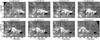 |
Fig. 1 Hα images of the active region NOAA 10763 obtained with the slit-jaw camera at the VTT. We can follow the evolution of the filament from the beginning of the observation at 14:38:33 to the end of the scan at 15:02:30. The drop-shaped dark feature in the lower-right part of the image is an artefact. The temporal evolution of the filament can be seen in a movie attached to the on-line edition. |
To facilitate the description of the filament movements, we show in Fig. 1 some of the simultaneous Hα images (with the UT time given at the top) obtained with the slit-jaw camera at the Vacuum Tower Telescope (VTT). A movie created from these and the remaining Hα slit-jaw images is available as electronic material. The images and the movie illustrate the very rapid evolution of the filament (darker structure) visible at the centre of the images in between the two flare ribbons (bright structures). The vertical line seen in the images is the slit of the spectrometer, while the two hairlines (horizontal lines) delimitate the field of view of the spectrometer. The black spot in the lower-right corner is an impurity on the mirror that holds the spectrograph slit. It does not affect our spectropolarimetric observations since it is only visible in the slit-jaw images. When we started our scan (upper leftmost image) a part of the filament material had already been ejected southward after the flare began at 14:34 (according to the GOES data). The filament initially moves before starting to rotate, possibly after a major reconnection event. The slit moves along the filament during the initial rising phase, but has just reached the right edge of the filament and moved on to the flare ribbons at the moment that it starts to display a rotating motion. Looking carefully at the movie, the rotation takes the form of a rolling motion (i.e. rotation around the axis of the flux rope), which is associated with filament material loosening itself from the main body of the filament and moving off to the sides. The impression we have from the movie is of an unwinding rope, of which one end has been released. Rolling motions in filaments have previously been noticed, for example, by Martin (2003), Panasenco et al. (2011), and Su & van Ballegooijen (2013). However, as indicated earlier, the recorded spectra are not expected to be influenced by the rotation. The filament does not erupt completely and we were unable to find evidence that it was associated with a coronal mass ejection.
The analysed data were recorded with the Tenerife Infrared Polarimeter TIP-II (Collados et al. 2007) mounted at the 70 cm aperture Vacuum Tower Telescope (VTT) at the Teide observatory in Tenerife. The filament was scanned in steps of 0.35′′ perpendicular to the slit orientation (180.51° with respect to the solar N-S direction), from 14:38:29 to 15:02:26 UT, providing a map of the region 36.5 × 25 Mm2 in size.
The reduction of the data has been described in Paper I. There we showed that the observed He Stokes profiles display a remarkably wide variety of shapes, and most of the profiles in the filament show very broad Stokes I absorptions and complex and spatially variable Stokes V signatures. The inversion of the profiles revealed multiple unresolved atmospheric blue- and redshifted components of the He i lines within a single-resolution element (~ 1 arcsec), with supersonic velocities of up to ~ 110 km s-1. Up to five different atmospheric components were found in the same profile, distinguished by their Doppler shifts, which generally differ by more than the sound speed. Note that each component is associated with a magnetic field. We demonstrated in Paper I that even these complex profiles can be reliably inverted.
The atmospheric parameters for the individual He components were retrieved by inverting the Stokes profiles, using the numerical code HeLIx+ (Lagg et al. 2004, 2009). The nine free parameters tuned by the code to fit the observed Stokes profiles were the magnetic field strength B and direction (inclination angle γ and azimuthal angle χ), the line-of-sight (LOS) velocity vLOS, the Doppler width ΔλD, the damping constant Γ, the ratio of the line centre to the continuum opacity η0, the gradient of the source function S1, and the filling factor αi, which defines the contribution of a given atmospheric component i to the total observed He profile. The sum of the filling factors of all atmospheric components within a resolution element is required to be unity, ∑ iαi = 1. We found that the most stable fits to the observed Stokes profiles were obtained by coupling the magnetic field strength B between the various Doppler-shifted He components, but leaving the two angles, γ and χ, of each line free. We also coupled the gradient of the source function S1 between the He atmospheric components. Coupling the field strength in the upper chromosphere is reasonable, because with increasing height in the solar atmosphere, the field becomes more homogeneous in strength and more diverse in direction (e.g. Solanki et al. 2006).
As explained in Paper I, the spectral region covered by the He absorption signature of strongly broadened or shifted profiles contains four photospheric lines (Si i at 10 827.09 Å, Ca i at 10 829.27 and 10 833.38 Å, and Na i at 10 834.85 Å). We had to fit these lines as well to obtain unbiased fits of the He i absorption, which often blends with some or all of these lines within the activated filament. Each photospheric spectral line was assigned its own atmospheric component and the spectropolarimetric inversions were made by coupling the magnetic field vector (B, γ and χ) and the gradient of the source function S1 between the photospheric lines, assuming that a single set of values approximately serves all four lines. This is consistent with the assumption that the four photospheric lines are formed at similar heights and can be represented by a single atmosphere. Among the photospheric lines, the Si i line is the strongest one with the best signal-to-noise ratio and shows clear signatures in the Stokes profiles. Changes in the atmospheric parameters will have a stronger influence on the Stokes profiles of the Si line than on the weaker photospheric lines. Therefore, the photospheric parameters are mainly determined by the shape and strength of the Si Stokes profiles. To obtain a good fit to the strong photospheric Si i line, we had to consider two atmospheric components: a magnetic component and a field-free stray-light component. Only this combination was able to satisfactorily reproduce both the line core and wings of the Si i line. We refer to Paper I for further details of the observations and the inversions.
For all the inverted profile, the vLOS of each atmospheric component was well retrieved with a small error. The inclination angle γ was retrieved with a somewhat larger error. Nonetheless, the inclinations of the different components of the magnetic field can often be clearly distinguished. The error bars on the azimuth angle, χ, were instead quite large, and it was often impossible to distinguish between the azimuths of the different magnetic components. This is mainly because of the complexity and the noise in the Q and U Stokes profiles. The information in the observations for retrieving the azimuth is limited. We therefore refrain from conclusions about the azimuthal direction of the magnetic field in the filament. Because of the unreliably determined magnetic azimuth we did not attempt to convert the magnetic vector from the observer’s frame of reference to local solar coordinates. Note that because Stokes V is generally much stronger than Q and U, Bcosγ is probably the most reliably determined quantity.
3. Results
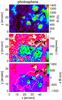 |
Fig. 2 Upper panel: map of the photospheric magnetic field strength determined from the photospheric lines. Middle panel: map of the photospheric magnetic field inclination with respect to LOS. Lower panel: map of the photospheric flux density. Red and white contours outline the border of the filament. The black arrow in the lower panel indicates the direction towards the centre of the solar disc. |
After inverting all the profiles at each pixel position of the map, it was possible to create maps of the more reliably retrieved atmospheric parameters to obtain a picture of the magnetic structure of the observed filament during its active phase.
First, we analysed the values obtained from the photospheric lines. Figure 2 displays maps of the magnetic field strength (upper panel), the magnetic field inclination angle with respect to the LOS (middle panel) and the flux density (αBcosγ, lower panel). Multiplying by the filling factor α, which weights the contribution of the magnetic component to the total profile of a photospheric line (see Sect. 2), ensures that we have the most reliably obtained quantity.
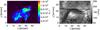 |
Fig. 3 Left: He intensity map obtained by integrating Ic − I over the wavelength covered by the He absorption (10 828–10 835.7 Å). The intensity contribution of the photospheric and telluric spectral lines in the chosen wavelength range has been subtracted. Right: Hα image obtained with the slit-jaw camera at the VTT at 14:22:33 UT. The contour line indicates the position of the inversion line of the magnetic field in the photosphere, that is, where γ = 90° (see Fig. 2). |
The contour line (red or white line) in Fig. 2 marks a total line absorption of I∗ = ∫(Ic − I)dλ equal to 2.0 × 10⁴ counts, where the integration runs over the wavelength range covered by the He absorption (10 828–10 835.7 Å). The intensity contribution of the photospheric and telluric spectral lines in the chosen wavelength range was subtracted to isolate the chromospheric absorption. The same contour was also superimposed on many of the following maps. It marks the boundary of the filament reasonably well, as seen in He i 10 830 Å. This can be judged from the left panel of Fig. 3, in which I∗ is plotted. Note that this outline traces the evolving filament as it was sampled by the moving slit. The average value of I∗ inside the filament is ≈3.5 times higher than the average value calculated in the quiet region around the filament. The highest value of the He absorption observed in the filament is ≈10 times higher than the He absorption in the quiet region.
In the middle panel of Fig. 2, we can clearly identify the position of the PIL where the magnetic field vector changes its polarity from outward (towards the observer, inclination angle close to 0°; green and blue) in the southern part of the scan to the opposite polarity (inclination angle close to 180°; pink and red) in the northern part. Figure 3 (right panel) displays an Hα image obtained with the slit-jaw camera at the VTT at 14:22:33 UT, prior to our scan and prior to the flare eruption. The filament mainly overlies the photospheric polarity inversion line (contour line drawn at γ = 90°, determined from the middle panel of Fig. 2). The horizontal black line is one of the hairlines marking the field-of-view of the TIP-II instrument. The filament contour in He i (obtained from the scan lasting from 14:42:16 to 14:56:54) only partly straddles the inversion line (see Fig. 2), unlike the filament seen in Hα at 14:22:33 (Fig. 3, right panel). The strong He absorption at least in the first part of the scan is clearly situated only above one polarity of the photospheric field, suggesting that the filament (or the flux rope structure) was evolving rapidly after activation by the flare. The movement of the material away from the photospheric inversion line is also deduced from the simultaneous Hα images obtained with the slit-jaw camera at the VTT (see Sect. 2).
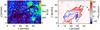 |
Fig. 4 Left: map of the chromospheric magnetic field strength. Right: map of the mean value of the retrieved vLOS for the He components weighted with the respective filling factor α. Red and black contours outline the position of the filament as sampled by the spectropolarimeter’s scan. They are defined as I∗ = ∫(Ic − I)dλ = 2 × 10⁴ counts (see left panel of Fig. 3). |
Figure 4 (left panel) displays the map of the retrieved chromospheric magnetic field strength. As explained in Sect. 2, we obtained the best fits to the observed Stokes profiles by coupling the magnetic field strength B between the He components. The field strength values are generally lower than 400 G inside the region of strong He absorption, which is indicated by the red contour line. Stronger-field regions correspond to the positions of small pores visible in the continuum intensity map (Fig. 1 in Paper I) and other prominent locations of strong field in the photosphere (Fig. 2). The average field strength in the filament ~119 G is lower than its average value in the region around it where is ~190 G. This difference probably reflects the fact that the He i line becomes optically thick inside the filament and is formed considerably higher than the surrounding atmosphere.
As a first impression, helpful for the He data interpretation and the discussion of the results presented in the next section, we show the overall chromospheric velocity pattern (Fig. 4, right panel). We calculated the weighted mean value of vLOS for each spatial pixel. The averaging was made over all atmospheric components deduced from the He-triplet inversions, weighted with their respective filling factors α. The downflows are mainly located at the edges of the filament (possibly corresponding to the footpoints), with the fastest ones at the right edge, while the upflows are mainly located in the body of the filament. As we noted in Sect. 2, the rolling of the filament occurs after the slit has left the filament. This is consistent with the absence of any preferred velocity pattern that would indicate a rolling filament in our resulting velocity maps.
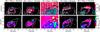 |
Fig. 5 Maps of the retrieved magnetic field inclination (γ, upper panels) and of the LOS magnetic field component (Bcosγ, lower panels) for the He components with retrieved LOS velocity in the range −60 < vLOS < −30 km s-1, −30 < vLOS < −10 km s-1, −10 < vLOS < 10 km s-1, 10 < vLOS < 30 km s-1, and 30 < vLOS < 110 km s-1. The contour line in the upper panels indicates the position of the PIL in the photosphere. The contour line in the lower panels traces the region of strong He absorption. |
Maps of the retrieved chromospheric magnetic field inclination with respect to the LOS are shown in the upper panels of Fig. 5. Inclinations for five ranges of LOS velocity are separated to distinguish between the inclinations retrieved from the different He components. The chosen vLOS ranges are −60 < vLOS < −30, −30 < vLOS < −10 (blueshifted components), −10 < vLOS < 10 (components nearly at rest), 10 < vLOS < 30, and 30 < vLOS < 110 km s-1 (redshifted components). Magnetic inclinations associated with these vLOS ranges are plotted from left to right in the upper panels of Fig. 5. If in one pixel multiple He components with vLOS in a given range coexist, we plot the inclination of the component with the highest filling factor. The contour line indicates the position of the apparent PIL in the photosphere, that is, where γ = 90° (see Fig. 2). The lower panels display the values of the LOS magnetic field in the atmospheric components within the different velocity bands, while the contour line traces the region of strong He absorption.
We first point out the general distribution of the signal in the different frames. This shows the locations of the regions with gas within the velocity ranges covered by the individual panels. Clearly, outside the filament there is only gas that is nearly at rest, with the exception of a few isolated locations of downflows with less than 30 km s-1. There is also a difference in the distribution of the most strongly upflowing and the most strongly downflowing gas (compare the leftmost with the rightmost panels). While the upflowing gas tends to be located in the body of the filament, the very rapidly downflowing gas is concentrated at its periphery. This confirms the general conclusion drawn from the right panel of Fig. 4. There is little spatial overlap between the fastest downflows and upflows.
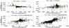 |
Fig. 6 LOS magnetic field component in the chromosphere versus the LOS magnetic field component in the photosphere for the He components with retrieved LOS velocity in the range −30 < vLOS < −10 km s-1 (top left), 30 < vLOS < 110 km s-1 (top right), and − 10 < vLOS < 10 km s-1 (bottom panels). The green lines represent linear regressions. |
We next consider the maps in the first and second columns of Fig. 5, that is, those derived from the blueshifted He components. These maps show a concentration of almost transversal field (γ ≈ 90°) between two regions of more longitudinal field lines with opposite polarities. The magnetic field vector points outward (towards the observer) in the northern part of the scan and inward in the southern part. The positions of the two polarities are opposite to those we retrieved in the photosphere, where the magnetic vector was instead pointing outward in the southern part of the scan and inward in the northern part. This behaviour is supported for the He components with −30 < vLOS < −10 km s-1 by Fig. 6, where we plot the LOS magnetic field component in the chromosphere versus the LOS magnetic field component in the photosphere for different He components (within specific velocity ranges). When the LOS magnetic field component in the photosphere is positive (pointing towards the observer), for the slower blueshifted He components (−30 < vLOS < −10 km s-1, top left panel), it appears to be negative in the chromosphere and vice versa (although the relationship is less clear in the other polarity, possibly due to LOS effects). The scatter plot for the range −60 < vLOS < −30 km s-1 does not show a clear relationship because of the displacement of the neutral line in the chromosphere with respect to the photosphere, which can be deduced from the top-left panel of Fig. 5. Hence, the same pixel in the photospheric and chromospheric map cannot be used to determine the correspondence in polarity. However, it is clear from the comparison of Fig. 2 with the leftmost panels of Fig. 5 that while the positive polarity in the photosphere is mainly concentrated on the south side of the filament, in the chromosphere the positive polarity is concentrated mainly to the north of the negative polarity.
From the maps in Figs. 2 and 5, we also notice that the photospheric field is more longitudinal than the chromospheric one, for which γ is more concentrated around the value of 90°. This result could reflect the situation on the Sun, but can also be an effect of the noise, since the signals in He are weaker than in Si. The resulting lower signal-to-noise ratios lead to the inversion code returning a less vertical field from the He lines than may actually be present in the upper chromosphere.
The panels of the third column of Fig. 5 depict the maps related to chromospheric gas almost at rest (−10 < vLOS < 10 km s-1). Outside the region covered by the filament, but also for the majority of the profiles observed in the filament, the magnetic field maintains the same polarities in both the photosphere and the chromosphere (see also the bottom panels of Fig. 6, left for the points inside the filament and right for the points outside). However, in some regions in the filament, in particular for 10″ < x < 25″, 3″ < y < 18″, the chromospheric magnetic field changes its polarity multiple times across the filament, while the photospheric field does not. Hence in this region the chromospheric field points in the opposite direction as compared to the photospheric magnetic field. This is only scarcely visible in Fig. 6 because Bcosγ is small at these locations.
The redshifted He components displayed in the fourth and fifth columns of Fig. 5 exhibit distributions of polarities of the magnetic field that resemble the photospheric pattern. The field lines run from outward (i.e. directed towards the observer) in the southern part of the scan to the opposite polarity in the northern part. This behaviour is confirmed by the scatter plot in the top-right panel of Fig. 6 for the fastest downflows: the LOS magnetic field components in the photosphere and in the chromosphere show a positive correlation, although with considerable scatter due to the mismatch of the PILs in the photosphere and chromosphere. In the range 10 < vLOS < 30 km s-1 the qualitative behaviour is the same as for the stronger redshifts, but (as for the profiles with −60 < vLOS < − 30 km s-1) the mismatch between the PILs in the photosphere and the chromosphere produces much scatter in a quantitative pixel-by-pixel comparison.
4. Discussion and conclusions
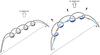 |
Fig. 7 First proposed scenario. Two of the magnetic field lines with different degrees of twist are plotted, which belong to the flux rope underlying the filament. At the left, the flux rope is in equilibrium, while at the right it rises. The filament material is represented by the shadowed regions, where the colours indicate whether the material is blue- or redshifted relative to the observer (who is located above the top of the image). The dashed line is the photospheric polarity inversion line. |
We have presented the, to our knowledge, first maps of the velocity and magnetic field of an activated filament in a flaring active region. The maps were created in both the photosphere and the chromosphere. Up to five different magnetic components were found in the chromospheric layers of the filament, while outside the filament a single component was sufficient to reproduce the observations. These components differ from each other in the gas flows they harbour and in the magnetic field inclination they have, and with different components deduced from the same set of Stokes parameters sometimes show opposite magnetic polarities.
The reliability of the deduced properties of these components was carefully discussed in Paper I. In addition, the reliability is also suggested, at least qualitatively, by the fact that the resulting maps of velocity and magnetic inclination are reasonably smooth and consistent, although individual profiles were inverted without using the values obtained from neighbouring profiles to guide the solution in any way (we recall that the HeLIx+ code makes use of a genetic algorithm that searches for the global minimum in the χ2 surface for every inverted profile).
These results suggest that the activated filament has a very complex structure. However, as we show below, this structure is compatible with a simple flux rope, although with a distorted one. In the following, we combine the information obtained from the inversions of the spectropolarimetric data to compare it with the different models of filament support. We find the best qualitative agreement of our observations with the flux rope model. In particular, this model explains the upflows and downflows well, showing opposite magnetic polarities within one and the same resolution element.
We summarise the main results obtained from the inversions. We measured downflow velocities of up to 110 km s-1 and upflows of up to 60 km s-1 along the LOS. These supersonic flows always coexist within the same resolution element with a component of the upper chromosphere almost at rest, or at least displaying a subsonic flow (−10 < vLOS < +10 km s-1). Upflows and downflows are both found throughout nearly the entire filament, with the following exceptions: at the end points of the filament (i.e. in its lower left and upper right corners) we see only fast downflows. They are associated with an almost longitudinal field with the same polarity as the underlying photospheric field. The central part of the filament mainly harbours upflows (although weaker downflows are present there as well). The blueshifted components of the He i triplet are in general associated with more transverse field lines, although closer to the edges of the filament the blueshifted gas is co-located with a more longitudinal field that has opposite polarities to the downflowing gas in the same pixels. This means that the upflowing gas is associated with opposite-polarity fields compared with the photosphere. We interpret this as signatures of the dips harbouring stable plasma in the rising flux rope.
The downflowing gas is therefore associated with more Ω-shaped field lines, while the upflowing gas appears to be carried by U-shaped field lines. How can this complex picture be reconciled with a filament model? From the sum of these observations we propose the following scenario:
Prior to its activation, the filament is described by an almost horizontal flux rope whose photospheric foot points are located at its lower-left and upper-right corners. Such low-lying filaments are typical for active regions (Zirin 1988; Martin 1990; Tandberg-Hanssen 1995). After this filament is activated, probably by the nearby flare, it starts to evolve rapidly, moving horizontally (see Hα images in Fig. 1 and the movie) and in particular rising, especially in the middle. This distorts the field. The axis of the flux rope, which originally was almost horizontal for most of the length of the filament (see the rough sketch of the filament before it was activated in the left frame of Fig. 7) becomes more curved, reaching higher in the centre, as indicated in the right image of Fig. 7. Later, possibly after a major reconnection event, the movie shows that the filament starts to roll (maybe unwinding). Unfortunately, we do not have spectropolarimetric information to support this interpretation, since the slit had just reached the right edge of the filament at the moment that it started to display this motion.
How do the observed down- and up-flows fit into this scenario? The magnetic field lines in a flux rope twist about its axis by one or multiple windings. The filament plasma comes to rest in the dips produced by these winding field lines. Note that field lines closer to the axis of the flux rope produce only shallow dips, where the filament plasma is more susceptible to perturbations, while field lines lying farther away from the axis have more pronounced dips, where the filament plasma is maintained more stably. In Fig. 7 we show a flux rope indicated by two representative field lines, one of them lying close to the flux rope axis (green line), the other farther away (black line). They both form dips, but possess different degrees of twist. When the flux rope is in equilibrium (left panel), the filament material, represented by the shadowed regions, rests inside the dips of both field lines. After the flux rope is destabilised and rises (right panel), the filament material still trapped inside the dips moves up with the whole flux rope. This is observed as upflows, which should be strongest near the centre of the rising flux rope according to the sketch. This material is trapped mainly in the outer, more twisted field lines. This rising material is associated with a field that displays the opposite polarity to the underlying photospheric field. However, near the footpoints of the flux rope the material may not be stably stored anymore, even in this outermost field line. It will flow down towards the legs. The magnetic polarity at such locations will be similar to that in the photosphere. Material bound to the less twisted inner field line cannot be maintained stably against gravity in the rising flux rope. It starts to flow down along the field line, contributing to the fast downflows at both footpoints of the filament. These downflows are associated with a chromospheric field that has the same polarity as the underlying photospheric field. This qualitative model can explain the coexistence of up- and downflows observed at the same spatial pixel positions as well as all the inclination of the magnetic field vectors associated with these flows.
Field lines with different degrees of twist are present in every flux rope (twisted flux tube). The twist increases from the inside out, with a completely untwisted field line in the centre, purely for symmetry reasons. Parker (1974, 1976) has described this structure, and for instance in the second order thin flux tube approximation (Pneuman et al. 1986; Ferriz-Mas et al. 1989) it is clearly seen that the magnetic field azimuth, χ, changes from zero at the axis to maximum at the edge. The green line in Fig. 7 is an integral part of every twisted flux tube model of a filament or prominence. Such a field line near the core of the flux rope can carry some of the mass, although much of the prominence mass will lie below it (unless the structure of the flux rope is similar to that described by Xu et al. 2012).
Other scenarios that reproduce our observations are also conceivable. One of these is based on the results of by Xu et al. (2012) and Kuckein et al. (2012b), who found plasma trapped both near the top and the bottom of the flux rope. Starting from a configuration similar to the one sketched in Fig. 10 of Xu et al. (2012) in the quiescent state, the activation and rise of the filament would lead to the draining of material from the shallower dips, that is, primarily from around the top of the flux rope (although material stored along the lower part of the more central field lines may also flow down the legs). All these and other conceivable scenarios have the disadvantage that they are more complicated than the one plotted in Fig. 7, and this added complexity does not a priori improve the reproduction of the observations. Therefore, following Occam’s razor, we concentrate here on the simplest model, plotted in Fig. 7.
This same behaviour, that is, upflows near the centre of the rising flux rope where plasma remains trapped in dips, and downflows for field lines that have lost their dips, has been found in recent simulations of the dynamics of cool plasma blobs in an erupting prominence (Su & van Ballegooijen 2013), although on a much larger scale.
An interesting point is that in addition to the supersonically flowing gas, we also found gas nearly at rest (or at least flowing only at subsonic speeds) throughout the filament. At least in the inner part of the filament this gas is associated with locally Ω-shaped field lines. The presence of this gas may suggest that not all field lines expand and bend as the filament becomes unstable. Some parts (possibly lower-lying ones) may have maintained their geometry.
Can we deduce the configuration from our observations? Low & Zhang (2002) proposed two different magnetic configurations of coronal flux ropes, one with the same sense of twist in the flux rope compared to the surrounding field (inverse configuration, see their Fig. 1), and another with the opposite sense of twist (normal configuration, their Fig. 2). Figure 2 shows that at the photospheric level the magnetic field points upward (has positive polarity) on the south-western side of the filament, and downward on the north-eastern side, so that the magnetic field overlying the flux rope is expected to move from SW to NE. However, the first two columns of Fig. 5 show that the blueshifted He components (the upward-moving material inside the flux rope) have positive polarity on the NE side of the flux rope and negative polarity on the SW side. This is opposite to the polarities of the surrounding field, as indicated by the photospheric measurements. This suggests that the observed filament has a sense of twist that is opposite to that of the surrounding arcade. Our observations are consequently more consistent with the normal configuration. From the analysis of the Hα images we can say that the flux rope is sinistral (referring to the direction of the component of magnetic field along the PIL as seen by an observer standing on the positive-polarity side of the filament, e.g., Martin et al. 1994). To be consistent with our results and conclusions, we show in Fig. 7 a sinistral left-helically twisted flux rope (the arrow on the black field line gives the sense of twist) following the normal configuration of Low & Zhang (2002).
Most prominences have an inverse configuration, not a normal one (Bommier et al. 1994). To our knowledge, the only evidence for flux ropes with normal configuration comes from Leroy’s measurements of magnetic fields in prominences above the limb and very recently from the works of Okamoto et al. (2008), Guo et al. (2010), and Kuckein et al. (2012a). Low & Zhang (2002) claimed that flux ropes with a normal configuration are responsible for fast coronal mass ejections from active regions.
Note that in the interpretations given above the plasmas with different LOS speeds within a single spatial resolution element are considered to be lying above each other (cf. Sasso et al. 2011). However, some of the plasma at different speeds may be at roughly the same height, for example, when turbulence or strong counterflows are present in the plasma of the activated prominence.
Online material
Movie of Figure 1 Access Supplementary Material
Acknowledgments
We thank Aad Van Ballegooijgen for reading a draft of this paper and generously providing suggestions. We thank the referee, Arturo López Ariste, for useful suggestions and comments. C.S. thanks the IMPRS on Physical Processes in the Solar System and Beyond for the opportunity to carry out the research presented in this paper. This work was supported by the ASI-INAF contract ASI N. I/013/12/0, Work Package 1310 – Operazioni Scientifiche. This work has been partially supported by the WCU grant No. R31-10016 funded by the Korean Ministry of Education, Science and Technology.
References
- Amari, T., Luciani, J. F., Mikic, Z., & Linker, J. 1999, ApJ, 518, 57 [Google Scholar]
- Andretta, V., & Jones, H. P. 1997, ApJ, 489, 375 [NASA ADS] [CrossRef] [Google Scholar]
- Antiochos, S. K., & Klimchuk, J. A. 1991, ApJ, 378, 372 [NASA ADS] [CrossRef] [Google Scholar]
- Antiochos, S. K., Dahlburg, R. B., & Klimchuk, J. A. 1994, ApJ, 420, 41 [Google Scholar]
- Aulanier, G., & Schmieder, B. 2002, A&A, 386, 1106 [NASA ADS] [CrossRef] [EDP Sciences] [Google Scholar]
- Aznar Cuadrado, R., Solanki, S. K., & Lagg, A. 2005, in Chromospheric and Coronal Magnetic Fields, eds. D. E. Innes, A. Lagg, S. K. Solanki, & D. Danesy (ESA Publication Division), ESA SP-596, 49 [Google Scholar]
- Avrett, E. H., Fontenla, J. M., & Loeser, R. 1994, in Infrared Solar Physics, ed. D. M. Rabin (Dordrecht: Kluwer Academic Publishers), IAU Symp., 154, 35 [Google Scholar]
- Babcock, H. W., & Babcock, H. D. 1955, ApJ, 121, 349 [NASA ADS] [CrossRef] [Google Scholar]
- Bommier, V., Landi Degl’Innocenti, E., Leroy, J. L., & Sahal-Bréchot, S. 1994, Sol. Phys., 154, 231 [NASA ADS] [CrossRef] [Google Scholar]
- Casini, R., López Ariste, A., Tomczyk, S., & Lites, B. W. 2003, ApJ, 598, 67 [Google Scholar]
- Charbonneau, P. 1995, ApJS, 101, 309 [NASA ADS] [CrossRef] [Google Scholar]
- Choe, G. S., & Lee, L. C. 1992, Sol. Phys., 138, 291 [NASA ADS] [CrossRef] [Google Scholar]
- Collados, M., Lagg, A., Díaz García, J. J., et al. 2007, in The Physics of Chromospheric Plasmas, eds. P. Heinzel, I. Dorotovič, & R. J. Rutten (San Francisco: ASP), ASP Conf. Ser., 368, 611 [Google Scholar]
- del Toro Iniesta, J. C. 2003, Introduction to Spectropolarimetry (Cambridge: Cambridge University Press) [Google Scholar]
- Ferriz-Mas, A., Schüssler, M., Anton, V. 1989, A&A, 210, 425 [NASA ADS] [Google Scholar]
- Gaizauskas, V., Mackay, D. H., & Harvey, K. L. 2001, ApJ, 558, 888 [NASA ADS] [CrossRef] [Google Scholar]
- Gibson, S. E., & Low, B. C. 1998, ApJ, 493, 460 [NASA ADS] [CrossRef] [Google Scholar]
- Gilbert, H. R., Holzer, T. E., & Burkepile, J. T. 2001, ApJ, 549, 1221 [NASA ADS] [CrossRef] [Google Scholar]
- Grossmann-Doerth, U., Schüssler, M., & Solanki, S. K. 1989, A&A, 221, 338 [NASA ADS] [Google Scholar]
- Guo, Y., Schmieder, B., Démoulin, P., et al. 2010, ApJ, 714, 343 [NASA ADS] [CrossRef] [Google Scholar]
- Heinzel, P. 2007, in The Physics of Chromospheric Plasmas, eds. P. Heinzel, I. Dorotovič, & R. J. Rutten (San Francisco: ASP), ASP Conf. Ser., 368, 275 [Google Scholar]
- Hyder, C. L. 1965, ApJ, 141, 1374 [NASA ADS] [CrossRef] [Google Scholar]
- Jensen, E. 1990, in Dynamics of Quiescent Prominences, eds. V. Ruzdjak, & E. Tandberg-Hanssen (New York: Springer-Verlag), IAU Colloq., 363, 129 [Google Scholar]
- Kippenhahn, R., & Schlüter, A. 1957, Z. Astrophys., 43, 36 [Google Scholar]
- Kuckein, C., Centeno, R., Martínez Pillet, V., et al. 2009, A&A, 501, 1113 [NASA ADS] [CrossRef] [EDP Sciences] [Google Scholar]
- Kuckein, C., Martínez Pillet, V., Centeno, R. 2012a, A&A, 539, A131 [NASA ADS] [CrossRef] [EDP Sciences] [Google Scholar]
- Kuckein, C., Martínez Pillet, V., Centeno, R. 2012b, A&A, 542, A112 [NASA ADS] [CrossRef] [EDP Sciences] [Google Scholar]
- Kuperus, M., & Raadu, M. A. 1974, A&A, 31, 189 [NASA ADS] [Google Scholar]
- Kuperus, M., & Tandberg-Hanssen, E. 1967, Sol. Phys., 2, 39 [NASA ADS] [CrossRef] [Google Scholar]
- Lagg, A., Woch, J., Krupp, N., & Solanki, S. K. 2004, A&A, 414, 1109 [NASA ADS] [CrossRef] [EDP Sciences] [Google Scholar]
- Lagg, A., Woch, J., Solanki, S. K., & Krupp, N. 2007, A&A, 462, 1147 [NASA ADS] [CrossRef] [EDP Sciences] [Google Scholar]
- Lagg, A., Ishikawa, R., Merenda, L., et al. 2009, in The Second Hinode Science Meeting, eds. B. Lites, M. Cheung, T. Magara, J. Mariska, & K. Reeves (San Francisco: ASP), ASP Conf. Ser., 415, 327 [Google Scholar]
- Landi Degl’Innocenti, E., & Landolfi, M. 2004, Polarization in Spectral Lines (Dordrecht: Kluwer Academic Publishers) [Google Scholar]
- Leroy, J. L. 1989, in Dynamics and Structure of Quiescent Solar Prominences, ed. E. R. Priest (Dordrecht: Kluwer Academic Publishers), 77 [Google Scholar]
- Leroy, J. L., Bommier, V., & Sahal-Bréchot, S. 1983, Sol. Phys., 83, 135 [Google Scholar]
- Leroy, J. L., Bommier, V., & Sahal-Bréchot, S. 1984, A&A, 131, 33 [NASA ADS] [Google Scholar]
- Lin, H., Penn, M. J., & Kuhn, J. R. 1998, ApJ, 493, 978 [NASA ADS] [CrossRef] [Google Scholar]
- López Ariste, A., & Aulanier, G. 2007, in The Physics of Chromospheric Plasmas, eds. P. Heinzel, I. Dorotovič, & R. J. Rutten (San Francisco: ASP), ASP Conf. Ser., 368, 291 [Google Scholar]
- López Ariste, A., & Casini, R. 2006, in Solar Polarization 4, eds. R. Casini, & B. W. Lites (San Francisco: ASP), ASP Conf. Ser., 358, 443 [Google Scholar]
- Low, B. C. 2001, J. Geophys. Res., 106, 25 [Google Scholar]
- Low, B. C., & Hundhausen, J. R. 1995, ApJ, 443, 818 [NASA ADS] [CrossRef] [Google Scholar]
- Low, B. C., & Zhang, M. 2002, ApJ, 564, 53 [Google Scholar]
- Low, B. C., & Zhang, M. 2004, ApJ, 609, 1098 [NASA ADS] [CrossRef] [Google Scholar]
- Martin, S. F. 1990, in Dynamics of Quiescent Prominences, eds. V. Ruzdjak, & E. Tandberg-Hanssen (Berlin: Springer), 1 [Google Scholar]
- Martin, S. F. 2003, Adv. Space Res., 32, 1883 [NASA ADS] [CrossRef] [Google Scholar]
- Martin, S. F., Bilimoria, R., & Tracadas, P. W. 1994, in Solar Surface Magnetism, eds. R. J. Rutten, & C. J. Schrijver (Dordrecht: Kluwer Academic Publishers), 303 [Google Scholar]
- Martínez Pillet, V., Collados, M., Sánchez Almeida, J., et al. 1999, in High Resolution Solar Physics: Theory, Observations, and Techniques, eds. T. R. Rimmele, K. S. Balasubramaniam, & R. R. Radick (San Francisco: ASP), ASP Conf. Ser., 183, 264 [Google Scholar]
- Okamoto, T. J., Tsuneta, S., Lites, B. W., et al. 2008, ApJ, 673, 215 [Google Scholar]
- Osherovich, V. A. 1989, ApJ, 336, 1041 [NASA ADS] [CrossRef] [Google Scholar]
- Panasenco, O., Martin, S., Joshi, A. D., & Srivastava, N. 2011, J. Atmos. Sol. Terrestr. Phys., 73, 1129 [NASA ADS] [CrossRef] [Google Scholar]
- Parker, E. N. 1974, ApJ, 191, 245 [NASA ADS] [CrossRef] [Google Scholar]
- Parker, E. N. 1976, Ap&SS, 44, 107 [NASA ADS] [CrossRef] [Google Scholar]
- Pécseli, H., & Engvold, O. 2000, Sol. Phys., 194, 73 [NASA ADS] [CrossRef] [Google Scholar]
- Penn, M. J. 2000, Sol. Phys., 197, 313 [NASA ADS] [CrossRef] [Google Scholar]
- Penn, M. J., & Kuhn, J. R. 1995, ApJ, 441, 51 [Google Scholar]
- Pneuman, G. W., Solanki, S. K., & Stenflo, J. O. 1986, A&A, 154, 231 [NASA ADS] [Google Scholar]
- Priest, E. R. 1990, in Dynamics of Quiescent Prominences, eds. V. Ruzdjak, E. Tandberg-Hanssen (Berlin: Springer), 150 [Google Scholar]
- Priest, E. R., Hood, A. W., & Anzer, U. 1989, ApJ, 344, 1010 [NASA ADS] [CrossRef] [Google Scholar]
- Rachkowsky, D. N. 1962, Izv. Krym. Astrofiz. Obs., 27, 148 [Google Scholar]
- Rachkowsky, D. N. 1967, Izv. Krym. Astrofiz. Obs., 37, 56 [Google Scholar]
- Roussev, I. I., Forbes, T. G., Gombosi, T. I., et al. 2003, ApJ, 588, 45 [Google Scholar]
- Rüedi, I., Solanki, S. K., & Livingston, W. C. 1995, A&A, 293, 252 [NASA ADS] [Google Scholar]
- Rust, D. M. 1967, ApJ, 150, 313 [NASA ADS] [CrossRef] [Google Scholar]
- Sasso, C., Lagg, A., & Solanki, S. K. 2006, A&A, 456, 367 [NASA ADS] [CrossRef] [EDP Sciences] [Google Scholar]
- Sasso, C., Lagg, A., & Solanki, S. K. 2011, A&A, 426, A42 [NASA ADS] [CrossRef] [EDP Sciences] [Google Scholar]
- Socas-Navarro, H., Trujillo Bueno, J., & Landi Degl’Innocenti, E. 2004, ApJ, 612, 1180 [Google Scholar]
- Socas-Navarro, H., Trujillo Bueno, J., & Landi Degl’Innocenti, E. 2005, ApJ, 160, 312 [Google Scholar]
- Solanki, S. K. 1993, Space Sci. Rev., 63, 1 [NASA ADS] [CrossRef] [Google Scholar]
- Solanki, S. K., & Stenflo, J. O. 1984, A&A, 140, 185 [NASA ADS] [Google Scholar]
- Solanki, S. K., Lagg, A., Woch, J., Krupp, N., & Collados, M. 2003, Nature, 425 [Google Scholar]
- Solanki, S. K., Inhester, B., & Schüssler, M. 2006, Rep. Prog. Phys., 69, 563 [NASA ADS] [CrossRef] [Google Scholar]
- Su, Y., & van Ballegooijen, A. 2013, ApJ, 764, 91 [Google Scholar]
- Tandberg-Hanssen, E. 1995, The Nature of Solar Prominences (Dordrecht: Kluwer Academic Publishers) [Google Scholar]
- Tang, F. 1987, Sol. Phys., 107, 233 [NASA ADS] [CrossRef] [Google Scholar]
- Trujillo Bueno, J. 2001, in Advanced Solar Polarimetry – Theory, Observation, and Instrumentation (San Francisco: ASP), ASP Conf. Ser., 236, 161 [NASA ADS] [Google Scholar]
- Trujillo Bueno, J. 2003, in Solar Polarization 3, eds. J. Trujillo Bueno, & Sanchez Almeida (San Francisco: ASP), ASP Conf. Ser., 307, 407 [Google Scholar]
- Trujillo Bueno, J., & Asensio Ramos, A. 2007, ApJ, 655, 642 [NASA ADS] [CrossRef] [Google Scholar]
- Trujillo Bueno, J., Landi Degl’Innocenti, E., Collados, M., Merenda, L., & Manso Sainz, R. 2002, Nature, 415, 403 [NASA ADS] [CrossRef] [PubMed] [Google Scholar]
- Unno, W. 1956, PASJ, 8, 108 [NASA ADS] [Google Scholar]
- van Ballegooijen, A. A. 2000, in Encyclopedia of Astronomy and Astrophysics, ed. P. Murdin (London: Institute of Physics Publishing), http://www.ency-astro.com [Google Scholar]
- van Ballegooijen, A. A., & Martens, P. C. H. 1989, ApJ, 343, 971 [NASA ADS] [CrossRef] [Google Scholar]
- Van Hoven, G., Mok, Y., & Drake, J. F. 1992, Sol. Phys., 140, 267 [NASA ADS] [Google Scholar]
- Wiegelmann, T., Lagg, A., Solanki, S. K., Inhester, B., & Woch, J. 2005, A&A, 433, 701 [NASA ADS] [CrossRef] [EDP Sciences] [Google Scholar]
- Wu, S. T., Bao, J. J., An, C. H., & Tandberg-Hanssen, E. 1990, Sol. Phys., 125, 277 [NASA ADS] [CrossRef] [Google Scholar]
- Xu, Z., Lagg, A., Solanki, S., & Liu, Y. 2012, ApJ, 749, 138 [NASA ADS] [CrossRef] [Google Scholar]
- You, J., Hui, L., Zhongyu, F., & Sakurai, T. 2001, Sol. Phys., 203, 107 [NASA ADS] [CrossRef] [Google Scholar]
- Zirin, H. 1988, Astrophysics of the Sun (Cambridge: Cambridge University Press) [Google Scholar]
All Figures
|
Fig. 1 Hα images of the active region NOAA 10763 obtained with the slit-jaw camera at the VTT. We can follow the evolution of the filament from the beginning of the observation at 14:38:33 to the end of the scan at 15:02:30. The drop-shaped dark feature in the lower-right part of the image is an artefact. The temporal evolution of the filament can be seen in a movie attached to the on-line edition. |
| In the text | |
|
Fig. 2 Upper panel: map of the photospheric magnetic field strength determined from the photospheric lines. Middle panel: map of the photospheric magnetic field inclination with respect to LOS. Lower panel: map of the photospheric flux density. Red and white contours outline the border of the filament. The black arrow in the lower panel indicates the direction towards the centre of the solar disc. |
| In the text | |
|
Fig. 3 Left: He intensity map obtained by integrating Ic − I over the wavelength covered by the He absorption (10 828–10 835.7 Å). The intensity contribution of the photospheric and telluric spectral lines in the chosen wavelength range has been subtracted. Right: Hα image obtained with the slit-jaw camera at the VTT at 14:22:33 UT. The contour line indicates the position of the inversion line of the magnetic field in the photosphere, that is, where γ = 90° (see Fig. 2). |
| In the text | |
|
Fig. 4 Left: map of the chromospheric magnetic field strength. Right: map of the mean value of the retrieved vLOS for the He components weighted with the respective filling factor α. Red and black contours outline the position of the filament as sampled by the spectropolarimeter’s scan. They are defined as I∗ = ∫(Ic − I)dλ = 2 × 10⁴ counts (see left panel of Fig. 3). |
| In the text | |
|
Fig. 5 Maps of the retrieved magnetic field inclination (γ, upper panels) and of the LOS magnetic field component (Bcosγ, lower panels) for the He components with retrieved LOS velocity in the range −60 < vLOS < −30 km s-1, −30 < vLOS < −10 km s-1, −10 < vLOS < 10 km s-1, 10 < vLOS < 30 km s-1, and 30 < vLOS < 110 km s-1. The contour line in the upper panels indicates the position of the PIL in the photosphere. The contour line in the lower panels traces the region of strong He absorption. |
| In the text | |
|
Fig. 6 LOS magnetic field component in the chromosphere versus the LOS magnetic field component in the photosphere for the He components with retrieved LOS velocity in the range −30 < vLOS < −10 km s-1 (top left), 30 < vLOS < 110 km s-1 (top right), and − 10 < vLOS < 10 km s-1 (bottom panels). The green lines represent linear regressions. |
| In the text | |
|
Fig. 7 First proposed scenario. Two of the magnetic field lines with different degrees of twist are plotted, which belong to the flux rope underlying the filament. At the left, the flux rope is in equilibrium, while at the right it rises. The filament material is represented by the shadowed regions, where the colours indicate whether the material is blue- or redshifted relative to the observer (who is located above the top of the image). The dashed line is the photospheric polarity inversion line. |
| In the text | |
Current usage metrics show cumulative count of Article Views (full-text article views including HTML views, PDF and ePub downloads, according to the available data) and Abstracts Views on Vision4Press platform.
Data correspond to usage on the plateform after 2015. The current usage metrics is available 48-96 hours after online publication and is updated daily on week days.
Initial download of the metrics may take a while.