| Issue |
A&A
Volume 561, January 2014
|
|
|---|---|---|
| Article Number | A39 | |
| Number of page(s) | 14 | |
| Section | Extragalactic astronomy | |
| DOI | https://doi.org/10.1051/0004-6361/201322081 | |
| Published online | 20 December 2013 | |
Ultraviolet to infrared emission of z > 1 galaxies: Can we derive reliable star formation rates and stellar masses?
1
Aix-Marseille Université, CNRS, LAM (Laboratoire d’Astrophysique de
Marseille) UMR7326, 13388
Marseille, France
e-mail:
This email address is being protected from spambots. You need JavaScript enabled to view it.
2
Department of Astronomy CSS Bldg., Rm. 1204, Stadium Dr.
University of Maryland College Park, MD 20742-2421,
USA
3
University of Crete, Department of Physics and Institute of
Theoretical & Computational Physics, 71003
Heraklion,
Greece
4
IESL/Foundation for Research & Technology-Hellas,
71110
Heraklion,
Greece
5
Observatoire de Paris, LERMA (CNRS: UMR8112), 61 Av. de
l’Observatoire, 75014
Paris,
France
6
Institut d’Astrophysique de Paris, UMR 7095, CNRS, UPMC Univ. Paris 06,
98bis
Boulevard Arago, 75014
Paris,
France
7
Institute for Astronomy, University of Hawaii,
Honolulu,
HI, 96822, USA
8
Canada-France-Hawaii telescope, Kamuela, HI, 96743,
USA
Received: 14 June 2013
Accepted: 9 October 2013
Abstract
Aims. Our knowledge of the cosmic mass assembly relies on measurements of star formation rates (SFRs) and stellar masses (Mstar), of galaxies as a function of redshift. These parameters must be estimated in a consistent way with a good knowledge of systematics before studying their correlation and the variation of the specific SFR. Constraining these fundamental properties of galaxies across the Universe is of utmost importance if we want to understand galaxy formation and evolution.
Methods. We seek to derive SFRs and stellar masses in distant galaxies and to quantify the main uncertainties affecting their measurement. We explore the impact of the assumptions made in their derivation with standard calibrations or through a fitting process, as well as the impact of the available data, focusing on the role of infrared emission originating from dust.
Results. We build a sample of galaxies with z > 1, all observed from the ultraviolet to the infrared in their rest frame. The data are fitted with the code CIGALE, which is also used to build and analyse a catalogue of mock galaxies. Models with different star formation histories are introduced: an exponentially decreasing or increasing SFR and a more complex one coupling a decreasing SFR with a younger burst of constant star formation. We define different sets of data, with or without a good sampling of the ultraviolet range, near-infrared, and thermal infrared data. Variations of the metallicity are also investigated. The impact of these different cases on the determination of stellar mass and SFR are analysed.
Conclusions. Exponentially decreasing models with a redshift formation of the stellar population zf ≃ 8 cannot fit the data correctly. All the other models fit the data correctly at the price of unrealistically young ages when the age of the single stellar population is taken to be a free parameter, especially for the exponentially decreasing models. The best fits are obtained with two stellar populations. As long as one measurement of the dust emission continuum is available, SFR are robustly estimated whatever the chosen model is, including standard recipes. The stellar mass measurement is more subject to uncertainty, depending on the chosen model and the presence of near-infrared data, with an impact on the SFR-Mstar scatter plot. Conversely, when thermal infrared data from dust emission are missing, the uncertainty on SFR measurements largely exceeds that of stellar mass. Among all physical properties investigated here, the stellar ages are found to be the most difficult to constrain and this uncertainty acts as a second parameter in SFR measurements and as the most important parameter for stellar mass measurements.
Key words: galaxies: high-redshift / galaxies: evolution / galaxies: photometry
Chercheur Associé.
© ESO, 2013
1. Introduction
Star formation rates (SFR) and stellar masses (Mstar) are the main parameters estimated from large samples of galaxies and they can be used to constrain their star formation history (SFH) and the evolution of their baryonic content. A large number of works found a tight relation between SFR and Mstar both at low and high redshift (e.g., Brinchmann et al. 2004; Daddi et al. 2007; Elbaz et al. 2007; Rodighiero et al. 2011), which is often called main sequence (MS) of galaxies (Noeske et al. 2007). The slope and the scatter of this relation as well as its evolution with redshift put constraints on the SFH of the galaxies as a function of their mass. The galaxies located on this MS may experience a rather smooth star formation evolution during several Gyr (Heinis et al. 2013) and the starburst mode seems to play a minor role in the production of stars (Rodighiero et al. 2011).
The degree to which we can interpret these observations depends on our ability to estimate SFR and Mstar. Two major methods (not independent) are commonly used to measure SFR and Mstar. The first approach consists of using empirical recipes. The SFR is deduced by applying conversion factors between an observed emission coming mostly from young stars and the SFR (e.g., Kennicutt 1998). The impact of dust attenuation has long been identified as a major issue. To overcome it, some calibrations combine different wavelengths and account for all the star formation directly observed in ultraviolet (UV)-optical or reprocessed in thermal infrared (IR; e.g., Hao et al. 2011; Kennicutt & Evans 2012; Calzetti 2012, and references therein). These relations rely on strong assumptions on SFH (Boissier 2013; Calzetti 2012), which are valid for local, normal galaxies, but may well break down for more extreme objects and at high redshift (Kobayashi et al. 2013; Schaerer et al. 2013). The Mstar estimations are also based on tabulated relations between mass to light (M/L) ratios and colors (e.g., Bell et al. 2003; Zibetti et al. 2009). The accuracy of their determination when rest-frame near-infrared (NIR) data are either included or not included remains an open issue: optical colors-M/L relations are less sensitive to the uncertain thermally pulsing asymptotic giant branch evolutionary phase, but the uncertainty due to dust reddening is strongly minimized in NIR (Conroy 2013, and references therein). The determination of SFR and Mstar is also strongly dependent on the choice of the stellar libraries and initial mass function (e.g., Bell et al. 2003; Muzzin et al. 2009; Marchesini et al. 2009).
Another widespread method to derive these physical parameters is to exploit the full panchromatic information available for a given sample by fitting the spectral energy distributions (SEDs). The first step is to model the stellar emission using an evolutionary population synthesis method, assuming a SFH with some recipes for dust attenuation. We then compare these theoretical SEDs to data. This method is particularly convenient when a large range of redshift is studied and when the wavelength coverage is wide. Without strong constraints on the amount of dust attenuation, an age-extinction degeneracy cannot be avoided (Pforr et al. 2012; Conroy 2013). In parallel to the development of models for the stellar emission, IR (>~5 μm) SEDs resulting from dust emission have been built and models have been developed that predict the full UV to IR SEDs of galaxies in a self-consistent manner for galaxies where most of the energy is produced by stars (da Cunha et al. 2008; Noll et al. 2009). The coupling of emissions both from stars and dust is physically due to the absorption of UV-optical photons by dust. The exact process of dust and star interaction is highly complex as it depends on many parameters, such as the dust grain composition and distributions, geometry, and age of the stellar populations (Popescu et al. 2011). At the scale of entire galaxies, it is impossible to model this process and the net effect of dust attenuation on the emission of a galaxy is usually described by an attenuation curve, the most popular one being that of Calzetti et al. (2000). The Mstar derivations are not sensitive to dust attenuation, but strongly depend on the assumed stellar population synthesis model and SFH (e.g., Papovich et al. 2001; Salim et al. 2007; Pforr et al. 2012; Maraston et al. 2010; Lee et al. 2009). For a given set of assumptions about the stellar population synthesis model, including metallicity and SFH, and adopting an initial mass function, the stellar masses can be estimated robustly. However, systematic differences appear when different assumptions are made and these input parameters are very poorly constrained (Muzzin et al. 2009). Marchesini et al. (2009) showed that these systematic uncertainties contribute at the same level as random errors in the derivation of stellar mass functions. The uncertainty about SFH itself induces large variations in stellar mass derivation (Bell et al. 2003; Lee et al. 2009; Pforr et al. 2012): the high luminosity of the young stellar population may hide an old stellar population. The effect can be very strong in bursty systems and leads to an underestimation of stellar ages (Maraston et al. 2010). As a consequence, stellar masses are likely to be more reliably measured in quiescent systems than in bursty galaxies (Wuyts et al. 2009; Pforr et al. 2012; Conroy 2013).
In this paper, we aim to measure the SFR and Mstar in a consistent way using different assumptions about SFH and different wavelength coverages. We focus on galaxies with a redshift larger than 1, which are intensively forming stars. Our analysis is based on a unique stellar population synthesis model (Maraston 2005). We refer to Conroy & Gunn (2010) for a comparison of the most popular population synthesis models in the framework of SED modelling. Numerous papers have been published to explore the reliability of SED fitting techniques, most of which are based on artificial catalogues of galaxies drawn from semi-analytical models or hydrodynamical codes (Wuyts et al. 2009; Lee et al. 2009; Pforr et al. 2012; Pacifici et al. 2012; Mitchell et al. 2013). These studies are all based on UV-optical and NIR data, but do not include IR emission. Our approach is somewhat different and complementary to these previous studies. First, we consider the whole electromagnetic spectrum from the UV to the IR and we estimate dust attenuation by balancing the energy absorbed by the dust in the UV/optical to the energy re-emitted in the thermal infrared. The strong constraints put on dust attenuation are expected to reduce the uncertainty of recent SFH retrieved by the SED fitting process. We combine true data and mock catalogues built with our fitting code. The priors of our artificial sources created with the fitting code are well defined and completely known, and their influence can be analysed at the price of over-simplistic modelling. Models based on semi-analytical codes or hydrodynamical simulations are certainly more realistic, but also depend on the assumptions made to produce them and it is more difficult to quantify the influence of these priors on the results of the SED fitting analysis.
We work between z = 1 and z = 3 in order to sample the UV continuum and the dust emission well. All galaxies are detected in the IR and, in particular, at 24 μm. The choice of the redshift range is essentially motivated by the quality of the photometric data and the performance of the SED fitting code as described in Sects. 2 and 3.1. The dataset is described in detail in Sect. 2, with a particular attention paid to the sampling of the rest-frame UV continuum emission using a large number of intermediate band filters. These filters have been proven to be very effective in measuring photometric redshifts (Ilbert et al. 2009; Benitez et al. 2009; Cardamone et al. 2010) as well as in characterising the dust attenuation (Buat et al. 2011, 2012) but, to our knowledge, their influence in retrieving physical parameters has not been studied yet. The fitting process, based on our modelling code, CIGALE (Noll et al. 2009), is presented in Sect. 3 along with the adopted star formation models and the determination of the main physical parameters (SFR, Mstar, and stellar ages). The influence of specific datasets (UV sampling, NIR, and IR) in the determination of these quantities are explored in Sect. 4. In Sect. 5 we generate mock catalogues and use them to explore possible systematic effects in the estimations of the physical parameters. Finally, our conclusions are presented in Sect. 6. We assume that Ωm = 0.3, ΩΛ = 0.7, and H0 = 70 km s-1 Mpc-1. The luminosities are defined in solar units with (L⊙ = 3.83 × 1033 erg s-1 and the adopted solar luminosity in the K band used to define M/LK ratios is 5.13 × 1032 erg s-1Hz-1 (corresponding to MK = 5.19 ABmag).
2. Observations and sample used
The Great Observatories Origins Deep Survey Southern (GOODS-S) field is among the best observed fields for the purpose of cosmological studies. Its wavelength coverage is exceptional, combining photometric observations from the UV to the IR1 and spectral surveys to measure as many redshifts as possible (Kurk et al. 2013, and reference therein). We select galaxies in this field with accurate measurements of the UV, visible, NIR, and IR rest frame emissions.
In the framework of the MUSYC project, Cardamone et al. (2010) compiled a uniform catalogue of multi-wavelength photometry for sources in GOODS-S, incorporating the GOODS Spitzer/IRAC and MIPS data (Dickinson et al. 2003). In addition to broadband optical data, they used deep intermediate-band (IB) imaging from the Subaru telescope to provide photometry with fine wavelength sampling and to estimate more accurate photometric redshifts. In a previous work, we used these data to trace the detailed shape of the UV rest-frame continuum and to perform an accurate measurement of the dust attenuation curve (Buat et al. 2011, 2012). As mentioned by Cardamone et al. (2010), the fluxes of extended sources may be underestimated in the MUSYC catalogue. The reason is that total fluxes are deduced from aperture fluxes using the SExtractor’s AUTO fluxes and a correction based on point source (stellar) growth curves. For extended sources this correction underestimates the total flux by a factor that depends on both the size and magnitude of the sources (as shown in Fig. 7 of Taylor et al. 2009). Our selection of sources with z > 1 ensures that we avoid this potential problem.
We restrict the field to the 10′ × 10′ observed by the PACS instrument (Poglitsch et al. 2010) on board the Herschel Space Observatory (Pilbratt et al. 2010) at 100 and 160 μm, as part of the GOODS-Herschel key programme (Elbaz et al. 2011). The GOODS-Herschel catalogue is obtained from source extraction on the PACS images performed at the prior position of Spitzer 24 μm sources, as described in Elbaz et al. (2011) and in the documentation provided with the data release2.
We start with the sources detected at 24 μm with a signal-to noise ratio (S/N) larger than 3 and we adopt the Spitzer/IRAC detections used to extract the 24 μm sources (Elbaz et al. 2011). These sources are cross-correlated with the MUSYC catalogue with a tolerance radius between the IRAC and optical coordinates equal to 1 arcsec. We further restrict the sample to sources that are not detected in the MUSYC X-ray catalogue of Cardamone et al. (2008). Our field corresponds to the very deep Chandra Deep Field-South survey (CDFS-S) reaching a limiting flux of 1.7 × 10⁻¹⁶ ergs-1 cm-2 in the 0.5−2 keV band (CDFS-S A03). We also select sources such that they have a single optical/UV counterpart within 3 arcsec. Particular care is given to the redshift of the sources: we select only galaxies of the MUSYC catalogue with a reliable spectroscopic redshift. All the spectra were taken with VLT spectrometers FORS and VIMOS. The quality of the redshift corresponds to more than 60% confidence level for the VIMOS surveys and labelled to be “high quality, secure, and likely” determinations for the FORS data (more detail can be found in the readme of the MUSYC catalogue and reference therein). As in Buat et al. (2012, hereafter Paper I), we consider only sources with at least two measurements at λ < 1800 Å in the rest frame of galaxies (broad or IB bands) with a S/N larger than 5. This condition ensures that we have a good definition of the UV continuum in the wavelength range mostly used to measure SFRs (1500−1600 Å) and for which calibrations are available in the literature. We obtain 312 galaxies that satisfy all these conditions. To combine the PACS observations with this sample we need to apply de-blending techniques to measure fluxes because of the large size of the PACS beam (Elbaz et al. 2011). We follow the prescription given in the documentation provided with the data release and only consider PACS measurements (with S/N > 3) for sources without bright neighbours defined as being brighter than half the flux density of the source and closer than 1.1 of the full width at half maximum (FWHM) of the point spread function (PSF). We add a further condition that no 24 μm bright neighbour must be found close to the 100 and 160 μm detections (i.e. no source brighter than half the flux density of the source at 24 μm and closer than 1.1 of the full width at half maximum (FWHM) of the point spread function (PSF) at 100 or 160 μm). In the end, we obtain 100 μm fluxes for 92 out of the 312 sources and 160 μm fluxes for 54. Finally, for z > 2, we only keep the sources detected with PACS since the 24 μm data correspond to rest frame wavelength lower than 8 μm and are not considered reliable to measure total IR emission from dust. With only two sources at z > 3, we reduce the sample to the 236 sources with 1 < z < 3. We detect 32 objects with PACS at 100 and 160 μm, 40 only at 100 μm, and eight only at 160 μm. The redshift distribution is shown in Fig. 1. We compile 28 photometric bands from U to 24 μm: the optical and NIR broadbands (U,U38,B,V,R,I,z,J,H,K), 13 IB bands from 427 to 738 nm, the four IRAC bands, and the MIPS1 24 μm band. We apply the revised IRAC selection criteria of Donley et al. (2012) to check that the 230 galaxies detected in the four IRAC bands all fall out of the AGN selection region defined in the f5.8/f3.6 and f8/f4.5 colour plot. The rest-frame luminosity at 1530 Å (corresponding to the far-UV (FUV) GALEX filter) of each galaxy is obtained by modelling a powerlaw, fλ(erg cm-2 s-1 Å-1) ∝ λβ between 1300 and 2500 Å, in the rest frame of the sources. In the following, we define LFUV as νLν at 1530 Å.
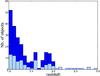 |
Fig. 1 Redshift distribution of the sources. The light blue histogram is for sources detected in at least one PACS filter. |
Input parameters for SED fitting with CIGALE.
3. SED fitting
The SED fitting is performed with the CIGALE code (Code Investigating GALaxy Emission)3 developed by Noll et al. (2009). The code CIGALE combines a UV-optical stellar SED with a dust component emitting in the IR and fully conserves the energy balance between the dust absorbed stellar emission and its re-emission in the IR. In the present work, we do not perform as detailed a study of dust attenuation as in Paper I. Instead, we keep the parameters of the attenuation curve (amplitude of the 2175 Å bump and slope of the UV attenuation curve) free since dust attenuation curves are expected to vary among galaxies (Witt & Gordon 2000; Inoue et al. 2006). We have checked that the estimated output parameters are fully consistent with the results obtained in Paper I. We adopt the stellar populations synthesis models of Maraston (2005), a Kroupa (Kroupa 2001) initial mass function (IMF), and a solar metallicity as our baseline. Different star formation histories are considered as described below.
Dust luminosities (LIR between 8 and 1000 μm) are computed by fitting Dale & Helou (2002) templates and are linked to the attenuated stellar population models: the stellar luminosity absorbed by the dust is re-emitted in the IR. The validity of Dale & Helou (2002) templates for measuring total IR luminosities of sources detected by Herschel is confirmed by the studies of Elbaz et al. (2010, 2011). A single parameter α describes these templates, defined as the exponent of the distribution of dust mass over heating intensity. When the source is detected in at least one PACS band, the input values of α are 1, 1.5, 2, and 2.5. As in Paper I, when PACS data are not available α is assumed to be 2, which corresponds to the average value found for galaxies detected with PACS. We have checked that the predicted fluxes in the PACS bands are consistent with a non-detection of these galaxies with PACS at a 3σ level quoted by Elbaz et al. (2011). The input parameter measuring dust attenuation is the attenuation in the V band (for the young stellar population if two stellar populations are involved), the input values used in this work are listed in Table 1. Dust attenuation in the FUV band is also defined as an output parameter of the code.
The parameters are all estimated from their probability distribution function (PDF) with the expectation value and its standard deviation, it is described as the “sum” method in Noll et al. (2009) and Giovannoli et al. (2011). In addition to the input parameters, the output parameters considered in this work will be Mstar, SFR, instantaneous and averaged over 100 Myr, ages of the stellar populations, and dust attenuation in the FUV (AFUV).
3.1. Star formation histories
We use different SFHs since we want to test their influence on parameter estimations. All the input parameters related to the SFH are listed in Table 1. Three scenarios are implemented in CIGALE and we consider all of them. Models are built with an age of creation of the first stars that can be either a free or fixed parameter. To fix the age of the stellar population we follow Maraston et al. (2010; see also Pforr et al. 2012) and adopt a redshift formation zf ≃ 8. Practically the whole redshift range is split to four intervals with different age models corresponding to a redshift formation of 8 for the central redshift of each interval (Table 1). The different SFH considered in this work are:
-
1.
A single stellar population with exponentially decreasing SFR and an e-folding rate τ1, called hereafter decl.-τ model. The age tf of the stellar population is left a free parameter since adopting a fixed age would be unrealistic for active star forming galaxies and would not produce reliable results. This model is still commonly used in the literature (Ilbert et al. 2013; Muzzin et al. 2013) although it has long been identified to be unrealistic (e.g., Boselli et al. 2001), leading to very young ages for the stellar populations (Maraston et al. 2010).
-
2.
A single stellar population with exponentially increasing SFR, called hereafter rising-τ model. The parameters are identical to those for the decl.-τ model, but with the age of the stellar population left either free or fixed. Several recent studies of distant galaxies prefer similar scenarios with rising SFR (Maraston et al. 2010; Papovich et al. 2011; Pforr et al. 2012; Reddy et al. 2012).
-
3.
Two stellar populations: a recent stellar population with a constant SFR on top of an older stellar population created with an exponentially declining SFR. The parameter tf is the age of the older stellar population, it is chosen to be either free or fixed. The age tySP of the young component is always a free parameter. The two stellar components are linked by their mass fraction fySP. Such models are introduced since they are expected to better reproduce real systems, which experience several phases of star formation (Papovich et al. 2001; Borch et al. 2006; Gawiser et al. 2007; Lee et al. 2009).
The complete grid of values is used to build the PDFs. In what follows we sometimes refer to Decl.-τ and rising-τ models as τ-models. For the two-populations model, a reduction factor of the visual attenuation, fatt, is applied to the old stellar population to account for the distributions of stars of different ages (Charlot & Fall 2000; Panuzzo et al. 2007). From our previous analyses, we adopt fatt = 0.5. The results are not sensitive to the exact value of this parameter.
More complex SFHs are also proposed in the literature. Delayed SFR (texp (−t/τ)) are not fully conclusive overall (e.g., Lee et al. 2010, 2011; Schaerer et al. 2013). More realistic histories derived from modelling of galaxy evolution combining power law and exponential variations (Buat et al. 2008; Behroozi et al. 2013) are promising. They are not yet implemented in CIGALE, but will be in its future version (Burgarella et al. in prep.). The treatment of emission lines is not optimal in the version of the code used in here. As a result we do not consider sources with z < 1 and those for which IB filters enter the rest-frame optical range where emission lines can have a large impact (Kriek et al. 2011; Schaerer et al. 2013).
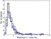 |
Fig. 2 Distributions of χ2 values obtained for the best fits and plotted in a logarithmic scale. Black: two-populations model, green: decl.-τ model, blue: rising-τ model. The solid lines are obtained for models with the age of the stellar population left free, the dashed lines correspond to a fixed age for the stellar population. |
3.2. Results of the spectral energy distribution fitting process
An initial, global, comparison of the three models of SFH can be performed by comparing the reduced best-fit χ2 distribution given by the code as shown in Fig. 2. Note that the derived physical parameters are not directly retrieved from the best model, but from the analysis of their probability distribution function calculated with all the input models. The number of degrees of freedom to calculate the reduced χ2 varies from 4 for the fixed-age τ-models to 7 for the free-age two-populations model. The best-fit χ2 distributions appear similar for all models. Best-fit χ2 values lower than 3 are found for more than ~90% of the sample with median value of χ2 equal to 1 for both fixed-age and free-age two-populations models and 1.3 for the one-population models (age-free decl.τ and age free and fixed rising-τ models). We conclude that the models considered reproduce our data satisfactorily with a slightly better fit obtained with the two-populations models.
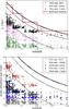 |
Fig. 3 Stellar ages estimated with CIGALE. Upper panel: ages of the (oldest) stellar population for free-age models as a function of redshift. Black triangles: two-populations model, green circles: decl.-τ model, magenta crosses: rising-τ model. The red steps correspond to the age adopted for the models with fixed ages. Lower panel: mass weighted ages for all the models: same symbols as in the upper panel are used for the free-age models, blue squares and red diamonds are added for the fixed-age rising-τ model and two-populations models, respectively. The curves correspond to the age at redshift z for a redshift formation zf = 8 (thick line), zf = 5 (thin line), and zf = 2.5 (dotted line). |
3.2.1. Stellar ages
In the upper panel of Fig. 3 we compare the ages tf when star formation begins, obtained for each model considered. The estimated ages are reported with the ones adopted for the fixed-age models. Very young and quite unrealistic ages for the beginning of the star formation are found with the free-age decl.-τ model. With the free-age rising-τ model the estimated ages are higher, yet remain quite low. It is an illustration of the well-known outshining of the young populations in galaxies forming stars actively as nicely illustrated by Maraston et al. (2010, their Fig. 12). Ages obtained with the free-age two-populations model are more realistic: combining a several billions-years-old population with a much more recent one (<300 Myr) gives more flexibility to account for the main light production by young stars with an underlying older population dominating the mass. The ages of the old population found with the free-age two-populations model correspond to a redshift formation from 2.5 (for galaxies at z = 1) to five (for galaxies at z = 2). If we assume that we are observing the same population of galaxies from z = 2−3 to z = 1, the age of the stellar populations found at different redshifts must be consistent: it is not the case for our free-age models. However, we may observe different galaxies at z = 1 and z = 2 since galaxies active in star formation at z = 2 may become quiescent at z = 1. Combining the average SFH Heinis et al. (2013) derive from the SFR-Mstar relation at different redshifts and assuming that galaxies exit the main sequence when they reach a mass characteristic of quiescent systems at the corresponding redshift, Heinis et al. (2013) estimate the time galaxies can stay on the main sequence. Galaxies with Mstar > 1010 M⊙ (which correspond to the bulk of our sample as shown in Sect. 3.2.2) located on the main sequence at z ≥ 2 reach their quenching mass before z = 1 and may well have evolved out of the main sequence. Heinis et al. (2013) also find that time spent on the main sequence decreases when Mstar increases.
The mass weighted age is also an output parameter of CIGALE. This age is representative of the average age of stellar populations. The values are reported in the lower panel of Fig. 3 as a function of redshift. The general trends are similar to those found in the upper panel with global shifts to lower ages. The free-age rising-τ and decl.-τ models lead to similar weighted ages whereas tf values were found to be larger for the free-age rising-τ models. For these models, the bulk of the stellar mass is built well after the beginning of the star formation. The fixed-age rising-τ model leads to slightly larger, but still very short, mass weighted ages.
The free-age decl.-τ models lead to very unrealistic ages, but we keep them, because of their popularity. Concerning the rising-τ models, the free-age option also leads to very young ages. Rising-τ models are commonly used by adopting a fixed formation redshift, which allows a high redshift formation with an average age for the bulk of the stellar population that remains young (Maraston et al. 2010; Papovich et al. 2011; Pforr et al. 2012). Therefore, we decided to keep only the fixed-age rising-τ model. For the two-populations models, the free-age option leads to plausible ages as discussed above, therefore we will keep both free-age and fixed-age models.
For the purpose of comparison between all these models, we adopt the free-age two-populations model as our baseline in the following.
3.2.2. Stellar mass and SFR determinations
Variation of the SFH:
SFR and Mstar estimates depend a priori on the assumed SFH. In this section, we consider the instantaneous SFR.
In Fig. 4, we compare Mstar values for all the models considered in this work, with our baseline model taken as the reference (x-axis). A good agreement is found with the rising-τ model with Δ(log (Mstar−ref.mod) − log (Mstar−rising − τ)) = 0.03 ± 0.08 dex. Substantial differences are found between the reference model and the same model with tf fixed: fixing the age of the oldest stellar population increases the stellar mass by 0.12 ± 0.04 dex. The lowest values of Mstar are found for the free-age decl.-τ models with Δ(log (Mstar−ref.mod) − log (Mstar−decl. − τ)) = 0.17 ± 0.09 dex. The difference between the extreme cases (free-age decl.-τ and fixed-age two-populations models) reaches 0.3 dex.
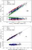 |
Fig. 4 Comparison of Mstar (upper panel) and SFR (lower panel) determinations from the different models. The x-axis is from the baseline model (free-age 2-populations), the y-axis corresponds to free-age decl.-τ (green circles), fixed-age rising-τ (blue dots), and two-populations (red diamonds) models. Typical uncertainties on parameter estimations are indicated by a black cross. Δ(SFR) = Δ(log (SFR2pop) − log (SFRτ − model)) and Δ(Mstar) = Δ(log (Mstar−2pop) − log (Mstar−rising − τ)). |
SFR determinations are much more consistent with each other. The agreement is almost perfect between both two-populations models. The star formation is dominated by the young stars formed in the more recent burst, which is fitted in the same way whether or not the age of the older population is free or fixed. A very slight shift towards higher SFR is found for the two-populations models as compared to the two other ones: Δ(log (SFR2pop) − log (SFRdecl. − τ)) = 0.04 dex and Δ(log (SFR2pop) − log (SFRrising − τ)) = 0.06 dex.
We confirm that the choice of the SFH changes the Mstar determinations significantly (Pforr et al. 2012). Because they are outshined by young stars, older stellar populations are hidden and τ- models are likely to give only lower limits to the total stellar mass (Papovich et al. 2001; Pforr et al. 2012). Models considering an old and young population are known to yield higher masses (Papovich et al. 2001; Borch et al. 2006; Lee et al. 2009; Pozzetti et al. 2007). The measurement of SFR are found to be robust against changes in the SFH. τ models yield results consistent with two-populations models with a constant star formation for the recent burst. Actually, Reddy et al. (2012) have shown that for ages larger than ~100 Myr rising-τ models lead to a constant production of the UV light. In the present study stellar populations are older than 2 Gyr for the rising-τ model, so we expect a robust determination of the SFR with the fit of the intrinsic UV continuum.
The effective SFH we obtain for the decl.-τ model is close to a constant SFR. The tf/τ ratio is always lower than unity and the age of the stellar population is larger than 100 Myr for 98% of our galaxies, ensuring a stationarity in the production of the UV light. Therefore we expected an agreement between our SFR estimations. The presence of IR data provides a robust measurement of the dust attenuation, allowing us to fit the true intrinsic UV continuum of our galaxies. The large impact of dust attenuation corrections will be discussed in Sects. 4 and 5.
Variation of the IMF:
throughout this paper we adopt a Kroupa IMF. CIGALE allows us to use a Salpeter IMF (Salpeter 1955). Several authors have studied the influence of the choice of the IMF on the SFR and Mstar determinations (e.g., Bell et al. 2003; Brinchmann et al. 2004; Pforr et al. 2012). We confirm that changing the IMF from Kroupa to Salpeter increases SFR and stellar masses by a constant factor found equal to 0.17 ± 0.01 dex and 0.21 ± 0.01 dex respectively, independent of the adopted SFH.
Variation of the metallicity:
throughout the paper we adopt a solar metallicity (Z⊙), but we can run CIGALE with Maraston models with Z⊙/2 and 2 Z⊙. The comparison of the SFR and Mstar determinations for these different metallicities are shown in Fig. 5. The values obtained with non-solar metallicities correlate very well with those obtained with Z⊙. A very small systematic shift is found for Mstar determinations, the stellar masses measured with a non-solar metallicity being lower than the reference metallicity by ~0.05 dex. This is likely due to the fact that stars in both sub-solar and super-solar models have slightly smaller turnoff masses (Maraston, priv. comm.). The effect is larger for SFR measurements in the case of super-solar metallicity. The SFR is increased by 0.20 dex for 2 Z⊙ models (and decreased by only 0.03 dex for Z⊙/2). This shift is attributed to a decrease of the UV photons for a given SFR in super-solar environment.
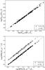 |
Fig. 5 Comparison of Mstar (upper panel) and SFR (lower panel) determinations for different metallicities. The quantities plotted on the x-axis are obtained with the baseline model assuming a solar metallicity, the y-axis corresponds to determinations with a half solar (dots) and twice solar (crosses) metallicity. |
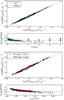 |
Fig. 6 Comparison between SFRIR,FUV (x-axis) and SFRSED (y-axis): the two upper panels are for τ-models, the two lower panels for the two-populations model, the difference between SFRSED and SFRIR,FUV is plotted against the age of the (youngest) stellar population. Symbols are the same as in Fig. 3. |
3.2.3. Star formation rate calibrations
We now compare the SFR found with our fitting method (SFRSED) to the one deduced directly from recipes converting FUV and IR luminosities into SFRs. The standard calibrations assume a constant SFR over ~108 years, which is sufficient to reach a stationary state for the UV production. Under this assumption, the intrinsic FUV luminosity is directly proportional to the current SFR. The total IR (~5−1000 μm) luminosity is related to the SFR by assuming that the bolometric emission of young stars is absorbed by dust and re-emitted in IR (Kennicutt 1998). Here we consider the total SFR as the sum of SFR obtained with the IR and FUV (not corrected for dust attenuation) luminosities. We do not account for heating of dust by older stars since all stellar populations are quite young. Buat et al. (2008) obtained a calibration for a Kroupa IMF and a constant SFR over 108 years. The observed FUV luminosity is calculated at 1530 Å and the total IR luminosity is integrated over the whole IR SED. It is an output of the CIGALE code, which is found independent on the assumed SFH. The SFR is calculated with the formula:  where the SFR is expressed in M⊙ yr-1 and the luminosities in L⊙.
The comparison between SFRIR,FUV and SFRSED is shown in Fig. 6. Both estimates are very consistent for τ-models since most of the sample stellar populations are older than 108 years with a SFH close to a constant one. There is a small shift between SFRIR,FUV and SFRSED for the two-populations model: the young population is younger than 108 years (tySP = 76 ± 38 Myr) and the UV production does not reach a fully steady production rate, leading to a slight underestimate of the instantaneous SFR with SFRIR,FUV. The difference is tightly correlated to tySP, the age of the young stellar population, but remains very modest on average (0.05 ± 0.03 dex) (Fig. 6, lower panel). The same effect is observed for decl.-τ models with very young stellar populations, leading to SFRSED larger than SFRIR,FUV (Fig. 6, upper panel). The few galaxies for which SFRSED < SFRIR,FUV correspond to objects with a very low mass fraction locked in the young stellar component (≃2%): the SFH is dominated by the decreasing old component, which is not constant over the last 108 years but, instead, has slightly decreased.
CIGALE also provides the SFR averaged over the last 100 Myr ⟨ SFR100 ⟩. The difference between ⟨ SFR100 ⟩ and SFRSED are plotted in Fig. 7 against the age of the (youngest) stellar population. For τ-models, the difference between the averaged and instantaneous SFR depends on the age of the stellar population and on the absolute value of e-folding rate τ, but the mean difference remains very small (−0.01 dex for the decl.-τ model, −0.03 dex for the rising-τ one). The situation is very different for the two-populations model: the difference between the averaged and instantaneous SFR strongly depends on the age of the young stellar population, which dominates the current star formation. The mean difference reaches −0.20 dex, but much larger differences can be found for individual objects. Very similar trends are found when SFRIR,FUV is used instead of the instantaneous SFR (not shown here). This clearly demonstrates that the SFR measured with UV and IR data, either with SED fitting or with empirical calibrations, are not equivalent to a SFR averaged over 100 Myr.
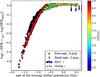 |
Fig. 7 Difference between the SFR averaged over 100 Myr and the instantaneous one given by CIGALE plotted as a function of the age of the youngest stellar population (tf for the τ-models and tySP for the two-populations model). Triangles are for the two-populations model, small circles for the rising-τ model and large circles for the τ model. The absolute value of the decreasing rate τ is color coded for τ-models. |
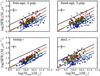 |
Fig. 8 SFR versus Mstar (left panels). Blue points z < 1.2, green diamonds 1.2 < z < 1.7, red squares 1.7 < z < 2, black triangles z > 2. From top to bottom: two stellar populations, one decreasing population, one increasing population models. The relations proposed by Elbaz et al. (2007) (blue, z ~ 1), Daddi et al. (2007) (red, z ~ 2), and Heinis et al. (2013) (green, z = 1.5, black z = 3) are over plotted with solid lines. |
3.3. Star formation rate-stellar mass relation
We have shown that the values of SFR and Mstar depend on the assumptions made to derive them. We now explore the consequences of these variations on the SFR-Mstar scatter plot. The SFR-Mstar relation is expected to evolve with redshift (e.g., Noeske et al. 2007; Wuyts et al. 2011; Karim et al. 2011). We split the sample into four redshift bins z < 1.2, 1.2 < z < 1.7, 1.7 < z < 2, and 2 < z < 3. The SFR and Mstar deduced from the SED fitting are plotted in Fig. 8. Very similar plots are found using SFRIR,FUV as expected from the very good correlation found between both SFR estimates. Different relations from the literature and covering our redshift range are overplotted: the relations of Elbaz et al. (2007) and Daddi et al. (2007) at z = 1 and 2 respectively, and the relations of Heinis et al. (2013) at z = 1.5 and 3.
Slight variations are seen between both two-populations and decl.-τ models, caused by the difference in Mstar measurements. The dispersion is large in all the scatter plots (except for the rising-τ model as discussed below) and we do not try to provide any relation. Our galaxy sample is built to have the best wavelength coverage, but is not complete in any sense and is not suited to derive a representative SFR- Mstar relation. Our selection of galaxies observed both in FUV and IR (rest-frame) is likely to bias towards objects with a high star formation activity. Free-age and fixed-aged two-populations models lead to a similar dispersion with a slight shift towards larger Mstar and lower specific SFR (SSFR) for the fixed-age model. Lower Mstar and similar SFR are obtained with the decl.-τ-model as compared to the results obtained with the other models and the discrepancy is larger when Mstar decreases (Sect. 3 and Fig. 4). It induces a flatter SFR-Mstar relation as compared to the other models. The residual rms error obtained with a linear fit for each redshift bin is ~0.3 for both two-populations and decl.τ models. The rising-τ model leads to a steeper, well-defined relation SFR-Mstar, which does not much evolve with redshift and the residual rms error to linear fits is reduced to ~0.2. This reduction is expected since rising SFHs have been introduced to explain the small scatter found in the SFR-Mstar relation and the non-evolution of the SSFR at very high redshift (Maraston et al. 2010; Papovich et al. 2011). This variation of the RMS error illustrates that the tightness of the derived SFR-Mstar relation also depends on the way these two quantities are derived.
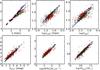 |
Fig. 9 Comparison between parameter estimations for the two-populations model with and without IB, NIR, and IR data. X-axis: all the dataset is used. Y-axis: parameters estimated without IB data (blue circles), without NIR data (green circles), and without IR data (red circles). |
4. Fitting spectral energy distributions with a reduced dataset
We now check the importance of the wavelength coverage to estimate our physical parameters. We identify three sets of data whose influence has to be investigated: the IB filters, sampling the UV continuum and sensitive to the recent SFH; the NIR rest frame data (K and all IRAC bands), often presented as the best tracers of Mstar; and the IR emission from dust sampled by IRAC4, MIPS, and PACS data, which is expected to provide a strong constraint to dust attenuation. We perform fits (i) omitting data obtained with all IB filters; (ii) omitting NIR data and (iii) omitting IR data. When one dataset is omitted, all the other data are kept. It may appear unrealistic from an observational point of view since galaxies detected in the IR are all detected with IRAC. Nevertheless, our aim is to test the influence of a specific wavelength domain on the determination of the physical parameters and to disentangle the different potential biases. The tests are performed for all SFH models, but are presented here for the two-populations model only. Similar trends are found for the other models.
In Fig. 9, the estimated values of the age of the stellar populations (tf and tySP), the mass fraction in the youngest population (fySP), the dust attenuation in FUV (AFUV), SFR and Mstar, obtained for cases (i); (ii); and (iii), are compared to those obtained with the full dataset (from Sect. 3). With CIGALE, the internal accuracy of the different parameter estimations is measured by the standard deviation of the probability distribution function of each parameter and for each object. The mean values of this standard deviation, averaged over the full sample of 236 galaxies are listed in Table 2 for each dataset.
All parameter estimates and the associated averaged dispersions are very similar with and without IB data, which play a minor role in these estimations. Only the values of tf are slightly larger without IB data, with no consequence in the determination of SFR and Mstar. We recall that the IB filters cover only the UV rest-frame range, which is essentially featureless. The situation is likely to be very different for IB sampling of the visible range with strong emission lines, which can strongly modify the overall spectrum (Schaerer et al. 2013). A good sampling of the UV continuum is useful to constrain the dust attenuation curve (Paper I) but does not add any useful information on the recent SFH provided that broadband photometry is available to measure the UV emission.
The decision of whether or not to include the NIR rest-frame data modifies most of the parameters, except AFUV and SFR, which are exclusively related to the young stellar population. We find moderate shifts for the ages of the stellar populations. When NIR data are excluded, tf is lower by up to 0.5 Gyr when tf > 2.5 Gyr and the young stellar populations are found to be 10% younger. The impact on the determination of Mstar is a small systematic shift, Mstar being lower by 15% on average when NIR data are excluded, with a dispersion reaching 0.16 dex between estimations with and without NIR data. The intrinsic uncertainty in the determination of Mstar also increases from 0.21 dex for the full dataset to 0.33 dex without NIR data.
Without IR data, results substantially change for all parameters linked to recent star formation. As expected, the parameters related to the old component (tf, Mstar) are much less affected. A substantial dispersion is observed in Fig. 9 between the values of tySP, fySP, SFR and AFUV, estimated with and without IR data (corresponding to 0.14 dex, 0.16 dex, 0.18 dex, and 0.44 mag, respectively). Looking at Table 2 it is clear that omitting IR data affects the accuracy of AFUV and SFR. The distribution of all these parameters is flatter without IR data and SFR are larger by 20% on average when IR data are excluded. This is illustrated in Fig. 10 with a dependence of the SFR estimates when IR data are not present on the SFR measured with the whole dataset. Under the assumption that SFR obtained with the whole dataset are reliable, in the absence of IR data, low SFR are overestimated and large SFR are underestimated, by a factor that can reach 2.5. The difference in SFR estimations strongly depends on the estimation of dust attenuation as seen in the lower panel of Fig. 10. If we assume that secure measurements are obtained when including IR data, large attenuations are underestimated implying an underestimation of the SFR, the inverse trend being observed for low attenuations. This is consistent with the conclusion of Burgarella et al. (2005, and erratum) that without IR data, the SED fitting process biases towards average values of dust attenuation.
Intrinsic uncertainty of the parameter estimation using the different datasets, measured as the dispersion of the probability function of each parameter.
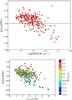 |
Fig. 10 Difference in SFR estimates when IR data are omitted. Upper panel: the SFR reported on the x-axis is calculated with the whole dataset. The Δ(log (SFR)) on the y-axis is defined as the log (SFR) (with the reduced dataset)-log (SFR) (with the whole dataset). Lower panel: Δ(log (SFR)) as a function of AFUV measured with the full dataset. The difference between AFUV is color coded. |
5. Mock galaxies
We checked the internal consistency and limitations of the method we used to retrieve physical quantities of galaxies. To this aim we built a sample of artificial SEDs defined in the same filters as those used for real sources. Then we attempted to retrieve the known properties of these pseudo-galaxies and to check the reliability of parameter estimation as well as the presence of potential systematic biases.
5.1. Definition of the mock catalogue with 1 <z < 2 and fitting process
Given the few sources with z > 2, we restrict the mock catalogue to 1 < z < 2. The actual redshift is not important since the models are only dependent on the physical ages of the stellar populations. The redshift range is introduced to reproduce data corresponding to the real sample and to account for the redshifting of the rest-frame emission of galaxies.
We only consider the free-age two-populations model. If we were to use all the parameters considered in Table 1 to simulate the artificial SEDs the total number of sources is very large and the computational time prohibitively long. Therefore, we restrict the sampling of the input parameters to the values appearing with bold characters in Table 1. We choose a single distribution of dust emission (α = 2), the dust attenuation law is fixed with parameters chosen from our previous study (Paper I). The sampling of the amount of dust attenuation is also reduced (but with the same total amplitude of variation), and we limit the mass fraction in the young stellar population to 20% at most. The SEDs are generated for all of the 30 bands (including the PACS bands) considered in this work, and a random noise, typically of the order of 10%, is added to the simulated fluxes. A similar, relatively small, error is applied to all the data since our aim is not to measure the effect of varying observational conditions, but to understand the limitations intrinsic to our modelling. All galaxies are created with a total galaxy mass of 1010 M⊙: we cannot check the dynamical range of SFR and Mstar but only systematic changes for these parameters. A total of 4970 artificial galaxies are created.
We fit the mock data, using CIGALE with the whole set of input parameters, as for real galaxies and not using the reduced set used to create the catalogue (cf. Table 1). We again perform again four distinct fits: using the whole dataset, excluding IB, NIR, or IR data. Note that when considering the influence of NIR rest-frame data we are not testing the role of the stellar population models since we are creating and fitting our artificial data with the same code.
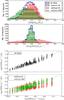 |
Fig. 11 Upper panels: histogram of the difference between the estimated values of Mstar and SFR and the exact values from the mock catalogue. Black line: whole dataset, blue line: without IB data, green filled histogram: without NIR data, red filled histogram: without IR data, Lower panel: SSFR estimated with SED fitting are compared to the true values of the SSFR. Black point: whole dataset, green dots: without NIR data, red dots: without IR data. Results without IB are not shown since they are indistinguishable from those without IR data. |
5.2. Stellar mass and SFR determinations
In Fig. 11 the difference between all the estimated and true values of SFR and Mstar are represented for the three combinations of data4. No effect on Mstar and SFR is found due to the lack of introduction of IB data, which confirms the findings with the real sample, the case without IB data will not be discussed. The impact of IR data is clearly seen, especially for the SFR determinations and the lack of introduction of NIR data modifies the Mstar distribution but in a much smaller amount than the IR data for the SFR.
When all the data are considered, there is only a small systematic difference between the estimated and true values of Mstar: ⟨ Δ(log (Mstar)) ⟩ = −0.07 dex with a 1σ dispersion equal to 0.14 dex. Without NIR data the systematic shift and the dispersion are larger: ⟨ Δ(log (Mstar)) ⟩ = −0.13 dex and σ = 0.20 dex. We confirm the difference of 15% found in Sect. 4.1, with and without NIR data for real galaxies.
The situation is worse for the SFR, when IR data are omitted: if the mean systematic difference, ⟨ Δ(log (SFR)) ⟩, remains consistent with 0, the dispersion varies from 0.05 dex with IR data to 0.30 dex without IR data. This poor determination of the SFR without IR data is clearly visible when SSFR are compared (lower panels of Fig. 11 ). We confirm that the range of values of SSFR found without IR data is reduced as compared to that of the true values, which are well estimated when IR data are considered. Intrinsically, small SSFR are overestimated without NIR data, this is due to underestimation of stellar masses for these objects, since SFR are well estimated in this case.
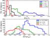 |
Fig. 12 Upper panel: distribution of the relative difference between the estimated and true age of the old stellar population. The sample is split as a function of the true age: tf = 1 Gyr, tf = 2 Gyr, tf = 3 Gyr, and tf = 4, 5 Gyr. Lower panel: distribution of the ratio of the estimated and true age of the young stellar population in logarithmic units. The sample is split as a function of the true age: tySP = 0.01 Gyr, tySP = 0.03 Gyr, tySP = 0.1 Gyr, and tySP = 0.3 Gyr. |
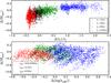 |
Fig. 13 Difference between estimated and true values of SFR and Mstar as a function of the difference between estimated and true ages. The colors are the same as in Fig. 12. |
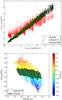 |
Fig. 14 Difference between estimated and true values of SFR as a function of the difference between estimated and true ages, dot are for fits with IR data, crosses correspond to fits without IR data. The difference between estimated and true values of AFUV is shown with a color scale. |
5.3. Stellar ages
We explored the different estimations of stellar ages, with and without IR and NIR data. We found very similar trends whether IR data are omitted or not. Therefore, in this sub-section, we begin by studying the fit with the whole dataset, and then we focus on the difference found between the fits with and without NIR data.
We have seen that the determination of the age of the stellar population is crucial to describing the SFH and to measuring Mstar, and that the impact on SFR is less important, as discussed in Sect. 3 and in the next sub-section. Our artificial sources are created with stellar populations spanning a large range of ages, between 1 and 5 Gyr for the old component and 0.01 to 0.3 Gyr for the young component. The relative difference between the estimated and true values of tf is shown in Fig. 12. Ages lower than ≃2 Gyr are overestimated (by 127% for tf = 1 Gyr and by 20% for tf = 2 Gyr) whereas larger ages are underestimated (by 16% for tf = 3 Gyr and by 30% for tf = 4 and 5 Gyr). The strongest discrepancy is found for the very small ages of the oldest stellar population. Lee et al. (2009) also found that the ages of model Lyman Break Galaxies , at z > 3 and lower than 1 Gyr, were strongly overestimated with SED fitting methods. We confirm that the ages of the old stellar populations are underestimated in typical galaxies with an old (>3 Gyr) underlying stellar population. The same effect is found for the age of the young stellar population.
These systematic shifts in age determination have a direct impact on Mstar measurements as shown in Fig. 13. Underestimations of tf and Mstar are correlated, which explains the large dispersion found in the Mstar distribution. The effect of tySP is less important, as expected, but the presence of a very young stellar population increases the uncertainty in the mass determination (Fig. 13, lower panel).
5.4. Dust attenuation
We have seen in Sect. 4 that dust attenuation has a major impact on SFR determinations. We re-investigate its role with our mock catalogue. The estimates of AFUV, with and without IR data, are compared in Fig. 14. Whereas dust attenuation is very well measured with IR data, when these IR data are missing AFUV is overestimated in systems with low attenuation and underestimated in very dusty systems, confirming the flattening of the distribution of AFUV found in Sect. 4 in the absence of observed IR data. It can be seen in Fig. 14 that dust attenuation plays a crucial role for SFR determinations whereas the age of the stellar population dominating the current SFR (tySP) only acts as a secondary parameter. When this age is overestimated the recent star formation is diluted over too large atimescale and the SFR is underestimated, as also found by Lee et al. (2009), but the effect remains very modest for our sample.
6. Conclusions
We measured SFR, Mstar, and stellar ages for a sample of 236 galaxies at 1 < z < 3 in the GOODS-S field observed with an excellent wavelength coverage, including UV and IR rest-frame data. We used 28 photometric bands from U to 24 μm, and 80 sources are detected with PACS at 100 or 160 μm. We also considered intermediate band (IB) filters which sample the UV rest-frame. We performed SED fitting with the code CIGALE, which implements an energy budget between dust and stellar emission. We explored different SFH: exponentially increasing and decreasing τ-models and a model combining an old decreasing SFR and a younger population of constant SFR. In a first step, the age of the main stellar population was left either fixed or free. The Decl.-τ models with a fixed redshift formation (zf ≃ 8) did not fit the data well. All the other models yield much better results at the price of young ages for free-age models, which were unrealistic with τ-models. The best fits are obtained with two-populations models. Ages were higher for the free-age two-populations model. In a second step, the models selected for the study were the free-age decl.τ model (because of its popularity), the fixed-age rising-τ model, and both fixed and free-age two-populations models. We investigated the impact of the coverage of different wavelength ranges. The analysis was also based on an artificial catalogue of 4970 sources built with the input parameters of the CIGALE code. Our main results can be summarized as follows:
-
1.
Instantaneous SFR are found independent of SFH assumptions with systematic differences lower than 10%. The instantaneous SFR measured by fitting the whole SED with τ-models are found fully consistent with SFRIR,FUV measured with empirical recipes, and 15% higher on average than SFRIR,FUV for the two-populations models, with a dependence on the age of the younger stellar population. The SFR averaged over 100 Myr and instantaneous SFR agree well for τ-models but not for the two-populations models.
-
2.
The stellar masses depend on the assumed SFH and are systematically lower by a factor of 1.5−2 for the decl.-τ model as compared to all the other models considered. It is caused by an obvious underestimate of the age of the stellar population for the free-age decl.τ model. Fixed-age rising-τ and free-age two-populations models are fully consistent with Mstar values lower on average by a factor of 1.3 than those obtained with the fixed-age two-populations model.
-
3.
The IB filters sample the UV rest-frame of our galaxies, which is almost featureless. As a consequence these data are found to play a minor role, if any, in the determination of SFR, Mstar as well as of stellar ages.
-
4.
Whether or not we include NIR and IR data modify parameter estimations substantially . With IR data, SFR are measured with a dispersion of 50%. Without IR data, the intrinsic dispersion reaches a factor of two and the range of estimated values is reduced when compared to the true values. The difference between estimations with and without IR is tightly correlated to the uncertainty of dust attenuation measurements. Excluding NIR data lowers Mstar estimates by 15% with an increase of the intrinsic dispersion from 60% with NIR data to a factor ~2 without them.
-
5.
Stellar age estimates are analysed with our mock catalogue. Systematic shifts are found: the shortest ages are overestimated and the largest ones underestimated with a direct impact on Mstar derivations, explaining the moderate systematic shift and dispersion found between the estimated and true values of Mstar. The impact of stellar age uncertainties on SFR measurements is much lower, SFR being far more sensitive to dust attenuation.
-
6.
These results have some impact on the SFR-Mstarrelation. The assumption of different SFH modifies the SFR-Mstar scatter plot. When two stellar populations are introduced, whether or not we fix the age of the oldest population has only a modest impact. The decl.-τ model leads to larger SSFR, especially for low-mass galaxies. The assumption of a rising SFH with a fixed age implies a well-defined SFR-Mstar which does not evolve much with z. A smaller range of SFR is found without IR data as well as a flatter variation of the SSFR than when IR data are introduced.
In Sect. 5, all the difference between the estimated and true values of a parameter are defined as “estimated value-true value”.
Acknowledgments
This work is supported by the French National Agency for Research (ANR-09-BLAN-0224) and CNES. The GOODS-Herschel data were accessed through the HeDaM database (http://hedam.lam.fr) operated by CeSAM and hosted by the Laboratoire d’Astrophysique de Marseille. The authors thank D. Elbaz, E. Daddi, and M. Bethermin for very fruitful discussions, and C. Maraston and J. Pforr for their help with stellar models. The anonymous referee’s suggestions have greatly helped the authors to improve the paper.
References
- Bell, E. F., McIntosh, D. H., Katz, N. & Weinberg, M. D. 2003, ApJS, 149, 289 [NASA ADS] [CrossRef] [Google Scholar]
- Benitez, N., Moles, M., Aguerri, J. A. L., et al. 2009, ApJ 692, L5 [NASA ADS] [CrossRef] [Google Scholar]
- Berhoozi, P., Wechsler, R., & Conroy, C. 2013, ApJ, 770, 57 [NASA ADS] [CrossRef] [Google Scholar]
- Boissier, S. 2013, in Planets, Stars and Stellar Systems. Vol. 6: Extragalactic Astronomy and Cosmology (Springer), 141 [Google Scholar]
- Borch, A., Meisenheimer, K., Bell, E., et al. 2006, A&A, 453, 869 [NASA ADS] [CrossRef] [EDP Sciences] [Google Scholar]
- Boselli, A., Gavazzi, G., Donas, J., & Scodeggio, M. 2001, AJ, 121, 753 [NASA ADS] [CrossRef] [Google Scholar]
- Brinchmann, J., Charlot, S., White, S. D. M. et al. 2004, MNRAS, 351, 1151 [NASA ADS] [CrossRef] [Google Scholar]
- Bruzual, G., & Charlot, S. 2003, MNRAS, 344, 1000 [NASA ADS] [CrossRef] [Google Scholar]
- Buat, V., Boissier, S., Burgarella, D., et al. 2008, A&A, 483, 107 [NASA ADS] [CrossRef] [EDP Sciences] [Google Scholar]
- Buat, V., Giovannoli, E., Heinis, S., et al. 2011, A&A, 533, A93 [NASA ADS] [CrossRef] [EDP Sciences] [Google Scholar]
- Buat, V., Noll, S., Heinis, S., et al. 2012, A&A, 545, A141 (Paper I) [NASA ADS] [CrossRef] [EDP Sciences] [Google Scholar]
- Burgarella, D., Buat, V. & Iglesias-Páramo, J. 2005, MNRAS, 360, 1413 [NASA ADS] [CrossRef] [Google Scholar]
- Calzetti, D. 2012, Proceedings of the XXIII Canary Islands Winter School of Astrophysics: Secular Evolution of Galaxies, eds. J. Falcon-Barroso, & J. H. Knapen [Google Scholar]
- Calzetti, D., Armus, L., Bohlin, R. C., et al. 2000, ApJ, 533, 682 [NASA ADS] [CrossRef] [Google Scholar]
- Cardamone, C. N., Urry, P. G., Damen, M., et al. 2008, ApJ, 680, 130 [NASA ADS] [CrossRef] [Google Scholar]
- Cardamone, C. N., van Dokkum, P. G., Urry, C .M., et al. 2010, ApJSS, 189, 270 [NASA ADS] [CrossRef] [Google Scholar]
- Charlot, S., & Fall, S. M. 2000, ApJ, 539, 718 [NASA ADS] [CrossRef] [Google Scholar]
- Conroy, C. 2013, ARA&A, 51, 396 [Google Scholar]
- Conroy, C., & Gunn, J. E. 2010, ApJ, 712, 833 [NASA ADS] [CrossRef] [Google Scholar]
- da Cunha, E., Charlot, S., & Elbaz, D. 2008, MNRAS, 388, 1595 [NASA ADS] [CrossRef] [Google Scholar]
- Daddi, E., Dickinson, M., Morrison, G., et al. 2007, ApJ, 670, 156 [NASA ADS] [CrossRef] [Google Scholar]
- Dale, D. A., & Helou, G. 2002, ApJ, 576, 159 [NASA ADS] [CrossRef] [Google Scholar]
- Dickinson, M., Giavalisco, M., & the GOODS team 2003, in The Mass of Galaxies at Low and High Redshift, eds. R. Bender, & A. Renzini (Springer), 324 [Google Scholar]
- Donley, J. L., Koekemoer, A. M., Brusa, M., et al. 2012, ApJ, 748, 142 [NASA ADS] [CrossRef] [Google Scholar]
- Elbaz, D., Daddi, E., Le Borgne, D., et al. 2007, A&A, 468, 33 [NASA ADS] [CrossRef] [EDP Sciences] [Google Scholar]
- Elbaz, D., Hwang, H. S., Magnelli, B., et al. 2010, A&A, 518, L29 [NASA ADS] [CrossRef] [EDP Sciences] [Google Scholar]
- Elbaz, D., Dickinson, M., Hwang, H. S., et al. 2011, A&A, 533, A119 [NASA ADS] [CrossRef] [EDP Sciences] [Google Scholar]
- Gawiser, E., Francke, H., Lai, K., et al. 2007, ApJ, 671, 278 [NASA ADS] [CrossRef] [Google Scholar]
- Giovannoli, E., Buat, V., Noll, S., Burgarella, D., & Magnelli, B. 2011, A&A, 525, A150 [NASA ADS] [CrossRef] [EDP Sciences] [Google Scholar]
- Finkelstein, F. S., Papovich, C., Salmon, B., et al. 2011, ApJ, 756, 164 [Google Scholar]
- Hao, C.-N., Kenniccutt, R. C., Jonhson, B. D., et al. 2011, ApJ, 741, 124 [NASA ADS] [CrossRef] [Google Scholar]
- Heinis, S., Buat, V., Bethermin, M., et al. 2013, MNRAS, in press [arXiv:1310.3227] [Google Scholar]
- Ilbert, O., Capak, P., Salvato, M., et al. 2009, ApJ, 690, 1236 [NASA ADS] [CrossRef] [Google Scholar]
- Ilbert, O., Salvato, M., Le Floc’h, E., et al. 2010, ApJ, 709, 644 [NASA ADS] [CrossRef] [Google Scholar]
- Ilbert, O., McCracken, H. J., Le Fevre, O., et al. 2013, A&A, 556, A55 [NASA ADS] [CrossRef] [EDP Sciences] [Google Scholar]
- Inoue, A., Buat, V., Burgarella, D., et al. 2006, MNRAS, 370, 380 [NASA ADS] [CrossRef] [Google Scholar]
- Karim, A., Schinnerer, E., Martínez-Sansigre, A., et al. 2011, ApJ, 730, 61 [NASA ADS] [CrossRef] [Google Scholar]
- Kennicutt, R. C. 1998, ARA&A, 36, 189 [Google Scholar]
- Kennicutt, R. C., & Evans, N. J. 2012, ARA&A, 50, 531 [NASA ADS] [CrossRef] [Google Scholar]
- Kobayashi, M. A. R., Inoue, Y., & Inoue, A. K. 2013, ApJ, 763, 3 [NASA ADS] [CrossRef] [Google Scholar]
- Kriek, M., van Dokkum, P. G., Whitaker, K. E., et al. 2011, ApJ, 743, 168 [NASA ADS] [CrossRef] [Google Scholar]
- Kroupa, P. 2001, MNRAS, 322, 231 [NASA ADS] [CrossRef] [Google Scholar]
- Kurk, J., Cimatti, A., Daddi, E., et al. 2013, A&A, 549, A63 [NASA ADS] [CrossRef] [EDP Sciences] [Google Scholar]
- Lee, S. K., Idzi, R., Ferguson, H. C., et al. 2009, ApJSS, 184, 100 [CrossRef] [Google Scholar]
- Lee, S. K., Ferguson, H. C., Somerville, R., Wiklind, T., & Giavalisco, M. 2010, ApJ, 725, 1644 [NASA ADS] [CrossRef] [EDP Sciences] [Google Scholar]
- Lee, K. S., Dey, A., Reddy, N., et al. 2011, ApJ, 733, 99 [NASA ADS] [CrossRef] [Google Scholar]
- De Lucia, G., Monaco, P., Somerville, R. S., & Santini, P. 2009, MNRAS, 397, 1776 [NASA ADS] [CrossRef] [Google Scholar]
- Maraston, C. 2005, MNRAS, 362, 799 [NASA ADS] [CrossRef] [Google Scholar]
- Maraston, C., Pforr, J., Renzini, A., et al. 2010, MNRAS, 407, 830 [NASA ADS] [CrossRef] [Google Scholar]
- Marchesini, D., van Dokkum, P. G., Förster Schreiber, N. M., et al. 2009, ApJ, 701, 1765 [NASA ADS] [CrossRef] [Google Scholar]
- Mitchell, P. D., Lacey, C. G., Baugh, C. M., & Cole, S. 2013, MNRAS, 1998 [Google Scholar]
- Muzzin, A., Marchesini, D., van Dokkum, P. G., et al. 2009, ApJ, 701, 1839 [NASA ADS] [CrossRef] [Google Scholar]
- Muzzin, A., Marchesini, D., Stefanon, M., et al. 2013, ApJ, 777, 18 [NASA ADS] [CrossRef] [Google Scholar]
- Noeske, K. G., Weiner, B. J., Faber, S. M., et al. 2007, ApJ, 660, L43 [Google Scholar]
- Noll, S., Burgarella, D., Giovannoli, E., et al. 2009, A&A, 507, 1793 [NASA ADS] [CrossRef] [EDP Sciences] [Google Scholar]
- Pacifici, C., Charlot, S., Blaizot, J., & Brinchmann, J. 2012, MNRAS, 421, 2002 [NASA ADS] [CrossRef] [Google Scholar]
- Panuzzo, P., Granato, G. L., Buat, V., et al. 2007, MNRAS, 375, 640 [NASA ADS] [CrossRef] [Google Scholar]
- Papovich, C., Dickinson, M., & Ferguson, H. C. 2001, ApJ, 559, 620 [NASA ADS] [CrossRef] [Google Scholar]
- Papovich, C., Finkelstein, s.L., Ferguson, H. C., Lotz, J. M., & Giavalisco, M. 2011, MNRAS, 412, 1123 [NASA ADS] [Google Scholar]
- Pforr, J., Maraston, C., & Tonini, C. 2012, MNRAS, 422, 3285 [NASA ADS] [CrossRef] [Google Scholar]
- Pilbratt, G., Riedinger, J. R., Passvogel, T., et al. 2010, A&A, 518, L1 [CrossRef] [EDP Sciences] [Google Scholar]
- Poglitsch, A., Waelkens, C., Geis, N., et al. 2010, A&A, 518, L2 [NASA ADS] [CrossRef] [EDP Sciences] [Google Scholar]
- Popescu, C. C., Tuffs, R. J., Dopita, M. A., et al. 2011, A&A, 527, A109 [NASA ADS] [CrossRef] [EDP Sciences] [Google Scholar]
- Pozzetti, L., Bolzonella, M., Lamareille, F., et al. 2007, A&A, 474, 443 [NASA ADS] [CrossRef] [EDP Sciences] [Google Scholar]
- Reddy, N., Pettini, M., Steidel, C., et al. 2012, ApJ, 754, 25 [NASA ADS] [CrossRef] [Google Scholar]
- Rodighiero, G., Daddi, E., Baronchelli, I., et al. 2011, ApJ, 739, L40 [NASA ADS] [CrossRef] [Google Scholar]
- Salim, S., Rich, R. M., Charlot, S., et al. 2007, ApJS, 173, 267 [NASA ADS] [CrossRef] [Google Scholar]
- Salpeter, E. E. 1955, ApJ, 121, 161 [Google Scholar]
- Schaerer, D., de Barros, S., & Sklias, P. 2013, A&A, 549, A4 [NASA ADS] [CrossRef] [EDP Sciences] [Google Scholar]
- Taylor, E. N., Franx, M., van Dokkum, P. G., et al. 2009, ApJ, 694, 1171 [NASA ADS] [CrossRef] [Google Scholar]
- Witt, A. N., & Gordon, K. D. 2000, ApJ, 528, 799 [Google Scholar]
- Wuyts, S., Franx, M., Cox, T., et al. 2009, ApJ, 696, 348 [NASA ADS] [CrossRef] [Google Scholar]
- Wuyts, S., Forster-Schreiber, N., Lutz, D., et al. 2011, ApJ, 738, 106 [NASA ADS] [CrossRef] [Google Scholar]
- Zibetti, S., Charlot, S., & Rix, H.-W. 2009, MNRAS, 400, 1181 [NASA ADS] [CrossRef] [Google Scholar]
All Tables
Intrinsic uncertainty of the parameter estimation using the different datasets, measured as the dispersion of the probability function of each parameter.
All Figures
|
Fig. 1 Redshift distribution of the sources. The light blue histogram is for sources detected in at least one PACS filter. |
| In the text | |
|
Fig. 2 Distributions of χ2 values obtained for the best fits and plotted in a logarithmic scale. Black: two-populations model, green: decl.-τ model, blue: rising-τ model. The solid lines are obtained for models with the age of the stellar population left free, the dashed lines correspond to a fixed age for the stellar population. |
| In the text | |
|
Fig. 3 Stellar ages estimated with CIGALE. Upper panel: ages of the (oldest) stellar population for free-age models as a function of redshift. Black triangles: two-populations model, green circles: decl.-τ model, magenta crosses: rising-τ model. The red steps correspond to the age adopted for the models with fixed ages. Lower panel: mass weighted ages for all the models: same symbols as in the upper panel are used for the free-age models, blue squares and red diamonds are added for the fixed-age rising-τ model and two-populations models, respectively. The curves correspond to the age at redshift z for a redshift formation zf = 8 (thick line), zf = 5 (thin line), and zf = 2.5 (dotted line). |
| In the text | |
|
Fig. 4 Comparison of Mstar (upper panel) and SFR (lower panel) determinations from the different models. The x-axis is from the baseline model (free-age 2-populations), the y-axis corresponds to free-age decl.-τ (green circles), fixed-age rising-τ (blue dots), and two-populations (red diamonds) models. Typical uncertainties on parameter estimations are indicated by a black cross. Δ(SFR) = Δ(log (SFR2pop) − log (SFRτ − model)) and Δ(Mstar) = Δ(log (Mstar−2pop) − log (Mstar−rising − τ)). |
| In the text | |
|
Fig. 5 Comparison of Mstar (upper panel) and SFR (lower panel) determinations for different metallicities. The quantities plotted on the x-axis are obtained with the baseline model assuming a solar metallicity, the y-axis corresponds to determinations with a half solar (dots) and twice solar (crosses) metallicity. |
| In the text | |
|
Fig. 6 Comparison between SFRIR,FUV (x-axis) and SFRSED (y-axis): the two upper panels are for τ-models, the two lower panels for the two-populations model, the difference between SFRSED and SFRIR,FUV is plotted against the age of the (youngest) stellar population. Symbols are the same as in Fig. 3. |
| In the text | |
|
Fig. 7 Difference between the SFR averaged over 100 Myr and the instantaneous one given by CIGALE plotted as a function of the age of the youngest stellar population (tf for the τ-models and tySP for the two-populations model). Triangles are for the two-populations model, small circles for the rising-τ model and large circles for the τ model. The absolute value of the decreasing rate τ is color coded for τ-models. |
| In the text | |
|
Fig. 8 SFR versus Mstar (left panels). Blue points z < 1.2, green diamonds 1.2 < z < 1.7, red squares 1.7 < z < 2, black triangles z > 2. From top to bottom: two stellar populations, one decreasing population, one increasing population models. The relations proposed by Elbaz et al. (2007) (blue, z ~ 1), Daddi et al. (2007) (red, z ~ 2), and Heinis et al. (2013) (green, z = 1.5, black z = 3) are over plotted with solid lines. |
| In the text | |
|
Fig. 9 Comparison between parameter estimations for the two-populations model with and without IB, NIR, and IR data. X-axis: all the dataset is used. Y-axis: parameters estimated without IB data (blue circles), without NIR data (green circles), and without IR data (red circles). |
| In the text | |
|
Fig. 10 Difference in SFR estimates when IR data are omitted. Upper panel: the SFR reported on the x-axis is calculated with the whole dataset. The Δ(log (SFR)) on the y-axis is defined as the log (SFR) (with the reduced dataset)-log (SFR) (with the whole dataset). Lower panel: Δ(log (SFR)) as a function of AFUV measured with the full dataset. The difference between AFUV is color coded. |
| In the text | |
|
Fig. 11 Upper panels: histogram of the difference between the estimated values of Mstar and SFR and the exact values from the mock catalogue. Black line: whole dataset, blue line: without IB data, green filled histogram: without NIR data, red filled histogram: without IR data, Lower panel: SSFR estimated with SED fitting are compared to the true values of the SSFR. Black point: whole dataset, green dots: without NIR data, red dots: without IR data. Results without IB are not shown since they are indistinguishable from those without IR data. |
| In the text | |
|
Fig. 12 Upper panel: distribution of the relative difference between the estimated and true age of the old stellar population. The sample is split as a function of the true age: tf = 1 Gyr, tf = 2 Gyr, tf = 3 Gyr, and tf = 4, 5 Gyr. Lower panel: distribution of the ratio of the estimated and true age of the young stellar population in logarithmic units. The sample is split as a function of the true age: tySP = 0.01 Gyr, tySP = 0.03 Gyr, tySP = 0.1 Gyr, and tySP = 0.3 Gyr. |
| In the text | |
|
Fig. 13 Difference between estimated and true values of SFR and Mstar as a function of the difference between estimated and true ages. The colors are the same as in Fig. 12. |
| In the text | |
|
Fig. 14 Difference between estimated and true values of SFR as a function of the difference between estimated and true ages, dot are for fits with IR data, crosses correspond to fits without IR data. The difference between estimated and true values of AFUV is shown with a color scale. |
| In the text | |
Current usage metrics show cumulative count of Article Views (full-text article views including HTML views, PDF and ePub downloads, according to the available data) and Abstracts Views on Vision4Press platform.
Data correspond to usage on the plateform after 2015. The current usage metrics is available 48-96 hours after online publication and is updated daily on week days.
Initial download of the metrics may take a while.