| Issue |
A&A
Volume 561, January 2014
|
|
|---|---|---|
| Article Number | A129 | |
| Number of page(s) | 19 | |
| Section | Astronomical instrumentation | |
| DOI | https://doi.org/10.1051/0004-6361/201321789 | |
| Published online | 22 January 2014 | |
The effects of spatial resolution on integral field spectrograph surveys at different redshifts − The CALIFA perspective
1 Centro Astronómico Hispano-Alemán, Calar Alto, (CSIC-MPG), C/Jesús Durbán Remón 2-2, 04004 Almería, Spain
e-mail: This email address is being protected from spambots. You need JavaScript enabled to view it.
2 Instituto de Astrofísica de Andalucía (CSIC), Glorieta de la Astronomía s/n, 18008 Granada, Spain
3 Instituto Nacional de Astrofísica, Óptica y Electrónica, Luis E. Erro 1, 72840 Tonantzintla, Puebla, Mexico
4 Departamento de Física Teórica, Universidad Autónoma de Madrid, 28049 Madrid, Spain
5 Leibniz Institute for Astrophysics Potsdam, an der Sternwarte 16, 14482 Potsdam, Germany
6 CEI Campus Moncloa, UCM-UPM, Departamento de Astrofísica y CC. de la Atmósfera, Facultad de CC. Físicas, Universidad Complutense de Madrid, Avda. Complutense s/n, 28040 Madrid, Spain
7 Institute of Astronomy, University of Cambridge, Madingley Road, Cambridge CB3 0HA, UK
8 CENTRA Centro Multidisciplinar de Astrofísica, Instituto Superior Técnico, Av. Rovisco Pais 1, 1049-001 Lisbon, Portugal
9 School of Physics and Astronomy, University of St Andrews, North Haugh, St Andrews KY16 9SS, UK
10 Instituto de Astrofísica de Canarias (IAC), Glorieta de la Astronomía S/N, 38206 La Laguna, S/C de Tenerife, Spain
11 Depto. Astrofísica, Universidad de La Laguna (ULL), 38206 La Laguna, Tenerife, Spain
12 Dep. Física Teórica y del Cosmos, Campus de Fuentenueva, Universidad de Granada, 18071 Granada, Spain
13 Centro de Astrofísica and Faculdade de Ciências, Universidade do Porto, rua das Estrelas, 4150-762 Porto, Portugal
14 Astronomisches Institut, Ruhr-Universität Bochum, Universitätsstr. 150, 44801 Bochum, Germany
15 RUB Research Department Plasmas with Complex Interactions, 44801 Bochum, Germany
16 University of Vienna, Türkenschanzstrasse 17, 1180 Vienna, Austria
17 Sydney Institute for Astronomy, School of Physics A28, University of Sydney, Sydney 2006 NSW, Australia
18 Australian Astronomical Observatory, PO Box 915, North Ryde NSW 1670, Australia
19 30 Department of Physics and Astronomy, Macquarie University, North Ryde NSW 2109, Australia
20 Max Planck Institute for Astronomy, Königstuhl 17, 69117 Heidelberg, Germany
Received: 29 April 2013
Accepted: 15 November 2013
Abstract
Context. Over the past decade, 3D optical spectroscopy has become the preferred tool for understanding the properties of galaxies and is now increasingly used to carry out galaxy surveys. Low redshift surveys include SAURON, DiskMass, ATLAS3D, PINGS, and VENGA. At redshifts above 0.7, surveys such as MASSIV, SINS, GLACE, and IMAGES have targeted the most luminous galaxies to study mainly their kinematic properties. The on-going CALIFA survey (z ~ 0.02) is the first of a series of upcoming integral field spectroscopy (IFS) surveys with large samples representative of the entire population of galaxies. Others include SAMI and MaNGA at lower redshift and the upcoming KMOS surveys at higher redshift. Given the importance of spatial scales in IFS surveys, the study of the effects of spatial resolution on the recovered parameters becomes important.
Aims. We explore the capability of the CALIFA survey and a hypothetical higher redshift survey to reproduce the properties of a sample of objects observed with better spatial resolution at lower redshift.
Methods. Using a sample of PINGS galaxies, we simulated observations at different redshifts. We then studied the behaviour of different parameters as the spatial resolution degrades with increasing redshift.
Results. We show that at the CALIFA resolution, we are able to measure and map common observables in a galaxy study: the number and distribution of H ii regions (Hα flux structure), the gas metallicity (using the O3N2 method), the gas ionization properties (through the [N ii]/Hα and [O iii]/Hβ line ratios), and the age of the underlying stellar population (using the D4000 index). This supports the aim of the survey to characterise the observable properties of galaxies in the Local Universe. Our analysis of simulated IFS data cubes at higher redshifts highlights the importance of the projected spatial scale per spaxel as the most important figure of merit in the design of an integral field survey.
Key words: techniques: spectroscopic / galaxies: abundances / stars: formation / galaxies: ISM / galaxies: stellar content
© ESO, 2014
1. Introduction
The Calar Alto Legacy Integral Field Area Survey (CALIFA, 0.005 < z < 0.03; Sánchez et al. 2012a) aims to characterise spectroscopically the galaxy population in the Local Universe, and on completion will be the largest and most comprehensive wide-field integral field spectrograph (IFS) survey carried out to date. With its statistically significant sample of ~600 galaxies, CALIFA will form the bridge between large single aperture surveys and detailed studies of individual galaxies.
Other surveys in the Local Universe using the power of integral-field spectrophotometers for a detailed study of nearby galaxies include the SAURON (Spectroscopic Areal Unit for Research on Optical Nebulae) project (de Zeeuw et al. 2002) and its extension ATLAS3D (z < 0.01; Cappellari et al. 2011), VENGA (VIRUS-P Exploration of Nearby Galaxies, Blanc et al. 2010), the DiskMass Survey (Bershady et al. 2010), and the PPAK IFS Nearby Galaxies Survey, PINGS (z ~ 0.002; Rosales-Ortega et al. 2010, hereafter RO10). Upcoming surveys are SAMI (Sydney Australian Astronomical Observatory Multi-object Integral Field Spectrograph, Croom et al. 2012) and MaNGA1 (Mapping Nearby Galaxies at APO, z ~ 0.05). At high redshift there is the SINS (Spectroscopic Imaging survey in the Near-infrared with SINFONI) survey (z ~ 2; Förster Schreiber 2009), the MASSIV (Mass Assembly Survey with SINFONI in VVDS) survey (z ~ 1; Vergani et al. 2012), the GLACE (GaLAxy Cluster Evolution) survey (z ~ 0.6; Sánchez-Portal et al. 2011), and the IMAGES (MAss Galaxy Evolution Sequence; z ~ 1; Ravikumar et al. 2007).
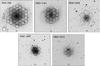 |
Fig. 1 Digital Sky Survey R-band images of the five galaxies selected from PINGS for this study (adapted from RO10). The IFS mosaicking is indicated by the superposition of the hexagonal PPak FoVs. Images are 10 × 10 arcmin2. North is up, east is to the left. |
In order to map the properties of local galaxies, a compromise must be made between the observing time invested on each object and the number of objects of the sample. The mosaicking approach designed for the PINGS survey, which mapped the H ii regions over the whole extension of the galaxies and explored the 2D metallicity structure of discs, involved more than 30 pointings and three years of observation. In contrast, the SAURON project opted for single pointings of the central part of early-type galaxies and bulges of spirals.
The CALIFA survey was designed with the aim of obtaining a balance between a detailed study of each galaxy and a statistically significant sample to fully characterise the optical properties of galaxies in the Local Universe. With this in mind, the sample was selected to have optical sizes that fit within the field of view (FoV) of the PPak instrument (PMAS – Potsdam Multi-Aperture Spectrophotometer – fiber pack, Roth et al. 2005; Verheijen et al. 2004; Kelz et al. 2006; Kelz & Roth 2006), allowing us to map their physical properties over their whole optical extent in just one pointing. In this context, one of the aims of the present paper is to determine the capability of CALIFA to measure the main properties of the observed galaxies despite resolution limitations.
Looking ahead to the next decade when new proposed surveys will explore the intermediate and high redshift regime, in this paper we also study how the information loss due to spatial resolution degradation will affect an hypothetical IFS survey at higher redshift. Taking advantage of the superb spatial sampling of a subsample of PINGS galaxies (z ~ 0.0009−0.0023, ≈0.04 kpc/arcsec), we create two simulations: simulation Z1 represents CALIFA at z ~ 0.02, and simulation Z2 represents an hypothetical survey at z ~ 0.05, or other redshift ranges depending on the instrument. In what follows, we refer to the PINGS redshift regime at an average z ~ 0.002 as Z0. We will analyse the behaviour of some common observables used in galaxy studies as the spatial resolution degrades with increasing redshift. Because of the low spectral resolution of PINGS data, we are unable to study the effect of spatial resolution on kinematics because the simulated cubes would not be representative of the higher spectral resolution CALIFA data.
Previous studies of this issue include Viironen et al. (2012) with a detailed study of UGC 9837 (z ~ 0.008863) repeating the analysis with simulated versions of the galaxy at higher redshifts (z ≈ 1 − 2). Kronberger et al. (2007) model disc galaxies using N-body/hydrodynamic simulations to investigate distortions in the velocity fields at different redshifts from z = 0 to z = 1. Giavalisco et al. (1996) simulate Hubble Space Telescope (HST) images at cosmological distances using images from the Ultraviolet Imaging Telescope (UIT), or the more recent work of Barden et al. (2008) where they simulate galaxies at redshifts 0.1 < z < 1.1 using images from the SDSS in the u, g, r, i, and z filter bands as input. Most of these studies have focussed on the degradation of images with redshift. Examples of studies focussing on spectral effects are Law et al. (2006) who mapped the velocity fields of high-redshift galaxies, and Yuan et al. (2013) who utilised the [N ii]/Hα ratio to investigate how an inferred metallicity gradient is altered by the loss of angular resolution.
The structure of this paper is as follows. In Sect. 2 we present the sample. Section 3 summarises the observations and data reduction while Sect. 4 explains how we simulate the different redshift regimes. The analysis of both gaseous and stellar components of the sample is presented in Sect. 5. In Sect. 6 we review the main results of this work.
Throughout this paper, we assume a standard ΛCDM cosmology consistent with WMAP results (Bennett et al. 2003) with Ωm = 0.3,ΩA = 0.7 and H0 = 70 h70 km-1 s-1.
2. Sample
The PINGS survey is a project designed to construct 2D spectroscopic mosaics of a representative sample of 17 nearby spiral galaxies, using PMAS in the PPak mode at the Centro Astronómico Hispano Alemán (CAHA) at Calar Alto, Spain. PINGS is one of the most detailed and largest IFS surveys of individual galaxies at low redshift (z ~ 0.001). The data cover most of the optical extent of the galaxies, down to R25 (the radius of the galaxy at the isophotal level of 25 mag/arcsec2 in B-band), with one of the best spatial resolutions and spectroscopic coverage achieved so far in any IFS survey. From the PINGS sample, we selected the five galaxies (Fig. 1) with the largest angular size (see Table 1 for details of each galaxy). The NGC 628 mosaic subtends 34 arcmin2 and was constructed from 34 different pointings, the NGC 1058 mosaic subtends 3.0 × 2.8 arcmin2 and was constructed from 7 different fields, the NGC 1637 mosaic was built from one central pointing and a concentric ring of 6 pointings covering a total area of 4.0 × 3.2 arcmin2, the NGC 3184 mosaic covers an area of 7.4 × 6.9 arcmin2 and was constructed from 16 IFS pointings, and finally the NGC 5474 mosaic covers an area of 4.8 × 4.3 arcmin2 and was built from of one central pointing and a concentric ring of 6 pointings.
PINGS subsample.
3. Observations and data reduction
The observations were carried out at the 3.5 m telescope of the Calar Alto observatory with the PMAS in the PPak mode. The PPak unit features a central hexagonal bundle with 331 densely packed optical fibres to sample an astronomical object with a resolution of 2.7′′/fibre, over an area of 74 × 65 arcsec2, with a filling factor of 65 % (<100% due to gaps in-between the fibres). The sky background is sampled by 36 additional fibres distributed in 6 mini-bundles of 6 fibres each, which encircle the central hexagon at a distance of ~90′′. All galaxies were observed using the same telescope and instrument set-up. The V300 grating was used, covering a wavelength range of 3700–7100 Å with a resolution of ~10 Å FWHM, corresponding to ~600 km s-1. The final product of the data reduction is a set of row-staked-spectra (RSS), a 2D FITS image where the X and Y axes contain the spectral and spatial information respectively, regardless of their position in the sky. An additional file links the different spatial elements to position on the sky. Row-staked-spectra present a discontinuous sampling of the sky, so we performed an interpolation to obtain a regularly sampled 3D cube (datacube). Not all PINGS datacubes have the same final sampling. NGC 1637, NGC 1058, NGC 3184 and NGC 5474 have 1′′/spaxel sampling, while NGC 628 has a sampling of 2′′/spaxel. For more details on the observing strategy, data reduction (similar to that used for the CALIFA data) and sample selection of the PINGS survey, see RO10.
4. Methodology
The aim of this work is to study how the loss of spatial resolution due to redshift affects the derivation of physical parameters obtained from IFS observations at different redshifts. We study three different spatial scales: (i) Z0 is at the original resolution of the PINGS data set, i.e. sampling of ~0.045 kpc/′′, or 80–100 spatial elements across the optical extent; (ii) Z1 is at the typical spatial resolution and sampling of a CALIFA galaxy of diameter ~60′′, with 25–30 spatial elements out to ~2–3 effective radii (Re); (iii) Z2 corresponds to a galaxy sampled at 1 kpc/′′ or ~7–10 spatial elements out to ~2–3 Re i.e. a z ~ 0.05 galaxy and instrument with ~1′′spatial elements. We should note that the key parameter is the number of spatial elements across the extent of the galaxy, the fiducial redshift of the galaxy will depend on the precise survey design. We then performed the same analysis on the three sets of galaxies (i.e. the original PINGS galaxies and both simulated sets) focusing on a set of commonly measured observables. In this way, we can quantify the extent to which we can recover observables of interest, and thus achieve the aim of characterising the properties of galaxies in the Local Universe, in both CALIFA and a hypothetical higher redshift IFS survey.
Spatial sampling at Z0, Z1 and Z2.
We decided to focus this study only on resolution effects, and in particular on spatial resolution degradation due to redshift. We have not considered either surface brightness dimming or increase in noise, i.e. we take for granted that the exposure time is sufficient to reach a similar depth in all cases. Also, we have not taken into account the effects of PSF, since, so far, the ability to spatially resolve a feature in an IFS dataset is more strongly affected by the sampling than by PSF size.
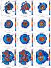 |
Fig. 2 V-band images constructed from the datacubes. Flux scale in arbitrary units. Left: original PINGS galaxies. Middle: Z1 galaxies. Right: Z2 galaxies. North is up, east is to the left. |
 |
Fig. 2 continued. |
4.1. Simulations
We binned the PINGS cubes using R3D to match the Z1 (CALIFA) sampling, and then binned again these cubes to match the Z2 sampling. Given an original cube of size Nx × Ny and a bin factor f, we add all the spectra in a box of size f × f and generate a new cube of size Nx/f × Ny/f. The spatial sampling detailed above results in f = 3 and f = 12 for all galaxies except for NGC 3184 where we used f = 2 and f = 8. As we are not considering noise, nor cosmological dimming, we consider the mean flux of the binned pixels, rather than integrating. In the absence of noise this will be statistically identical, and makes direct comparisons much easier. Table 2 gives the spatial sampling and fiducial redshift for each galaxy in the three surveys. To avoid binning artefacts such as border discontinuities, we applied a 2D Gaussian smoothing to the cubes after binning. This resembles the effects of an interpolation kernel passed over fibre-based (dithered or not) IFS observations. We have also tested convolution of the data before binning, more appropriate for regularly gridded observations, such as SINFONI, VIMOS, MUSE or GMOS. In all tests we obtained qualitatively similar, although quantitatively different, results. The differences do not affect the conclusions of this work in any way. Figure 2 shows V-band images of the original and simulated galaxies. The images are constructed by convolving a Johnson V-band filter with the datacubes.
5. Analysis
The aim of this paper is to understand how observed properties of H ii regions, in particular radial trends and spatial distribution, are affected by spatial resolution degradation. A complete analysis of the behaviour of derived properties and impact on physical conclusions will be the subject of forthcoming papers.
We performed a set of standard analyses of increasing complexity: (i) reconstruction of broad-band images from the IFS datacubes; (ii) creation of emission line flux maps; (iii) measurement of more complex spectroscopic properties, such as line ratios, chemical abundance tracers, and ionisation indicators, following the procedures described in Sánchez et al. (2012a,b).
To analyse the information contained in the cubes, we used FIT3D to separate the underlying stellar continuum from the emission lines in each spectrum, following the process described in detail in Sánchez et al. (2011) and RO10. FIT3D routines fit the underlying stellar population combining linearly a set of stellar templates within a multi-SSP model. A simple SSP template grid was adopted, consisting of three ages (0.09, 1.00 and 17.78 Gyr) and two metallicities (Z ~ 0.0004 and 0.03). The SSP templates were taken from the MILES project (Vazdekis et al. 2010). The metallicities and ages cover the wide ranges possible within the MILES library. The oldest stellar population was selected to reproduce the reddest possible underlying stellar population, mostly due to higher metallicities than the one considered in our simplified model, although it is clearly older than the accepted cosmological age of the Universe. Our youngest stellar population is the 2nd youngest in the MILES library for which both metallicities are available. No appreciable difference was found between using this or the youngest SSP (~80 Myr). Finally, we selected an average age stellar population, of ~1 Gyr, required to reproduce the intermediate-to-blue stellar populations, and to produce more reliable corrections of the underlying stellar absorption.
We study commonly used indicators of gaseous and stellar properties. In the case of the gas emission, these are the Hα flux, the [O iii]λ5007/Hβ vs. [N ii]λ6583/Hα BPT diagnostic diagram (Baldwin et al. 1981; Veilleux & Osterbrock 1987), and the radial oxygen abundance gradient derived from the widely-used O3N2 strong-line indicator (Pettini & Pagel 2004; Marino et al. 2013). For the stellar component we decided to show the 4000 Å break D4000 (i.e. the break strength at 4000 Å defined as the ratio of the average flux densities in the narrow bands 4000–4100 Å and 3850–3950 Å, Balogh et al. 1999) as it is the most commonly used proxy for mean stellar age.
All radial profiles are plotted in units of R25 obtained from the RC3 catalogue (de Vaucouleurs et al. 1992) and scaled to each redshift regime. Surface brightness profiles for each galaxy (Fig. 3) were constructed using the IRAF2 task ellipse and then scaled in the y-axis to make them coincide at Rmax/2 (maximum measured radius divided by 2), in order to analyse the profile differences between galaxies. For the ellipse fitting we used V-band images extracted from the datacubes as explained before.
All the above analyses (fitting and subtracting the underlying stellar continuum and fitting of the emission lines) were performed independently on each datacube, i.e both the original and simulated ones.
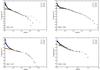 |
Fig. 3 Surface brightness profiles of the original PINGS galaxies and the simulated ones, constructed fitting ellipses to V-band images extracted from the datacubes. The profiles were scaled in the y-axis to make them coincide at Rmax/2 (maximum measured radius divided by 2). |
5.1. Morphology
From Fig. 2 we can see that at the representative redshift of CALIFA (Z1, middle panel) we are able to qualitatively reproduce most morphological features. In all cases we can trace the spiral arms, rings and bulge extension seen in the original images. Finer detail such as individual regions or spots, are smeared out on the Z1 case, so qualitatively we can see that the analysis of the distribution of some features along the arms or small regions will be limited by the resolution effect.
In the Z2 regime (Fig. 2, right panel), the situation is totally different. Except in the case of NGC 628, where, as a grand-design galaxy, the spiral arms are very well defined and still traceable to high redshift, in all other galaxies the identification of spiral signatures is hampered. Individual regions are not easily detected and the separation between the bulge and the disc becomes subtle. The latter effect can also be appreciated from the surface brightness profiles in Fig. 3. In all cases, the primary effect of spatial resolution loss is that the profiles become flatter in the centre. In the Z1 case the central component, though smoothed, can be detected as an excess of light above the inward extrapolation of the disc. That is not the case for the Z2 profiles where the inner regions are shallow and a single component fit to the data seems to be the best option, although a slight disc/bulge differentiation could be seen in the radial plots.
5.2. Ionized gas component
5.2.1. H ii region distribution
To extract the Hα intensity maps for all the cubes (see Figs. 4 and 5) we co-add the flux intensity within a square-shaped simulated filter centred at the wavelength of Hα (6563 Å) shifted to the observed frame considering the redshift of the object, with a width of 60 Å. The adjacent continuum for each pixel was estimated averaging the flux intensity within two bands on both sides of the centre, separated 100 Å from it and with a width of 60 Å. This continuum intensity is then subtracted from the Hα intensity to derive a continuum-subtracted emission line map. It is worth noting that this Hα intensity map is contaminated with the adjacent [N II] emission lines, and it is not corrected for Balmer absorption of the underlying stellar population.
Figure 4 show the resulting maps from the original and degraded datacubes. The Z1 maps show the same distribution of H ii regions tracing the spiral arms as in the Z0 case. Because of the coarse resolution, the H ii regions found in the Z1 case are complexes of several PINGS regions but without a severe alteration of Hα flux local maxima position. On the contrary, as can be expected from the global morphology noted in the previous section, the Hα 2D distribution in the Z2 simulation, presents a strong difference as many H ii complexes are averaged into one single Hα aggregation. Again, no traceable spiral arms are visible for the Z2 regime, and even in the NGC 628 case, in which the spiral structure is perfectly traced by the H ii complexes at Z0 and Z1, the Z2 galaxy presents a morphology that at a first sight it is not easily associated with a spiral structure. In any case, it is worth noting that the morphological analysis presented here is meant to show the effects of resolution in the morphology, in the understanding that any spectroscopic survey will have an imaging follow up to derive the morphology with better resolution and that kind of work will not be done from the line maps (although this might not be the case for all high-redshift studies, since some of them relies only in the IFS data).
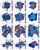 |
Fig. 4 Hα images extracted from the cubes. Flux is in units of 10-16 erg s-1 cm-2 Å-1. Z1 and Z2 are scaled to Z0 flux. Left: original Z0 galaxies. Middle: Z1 galaxies. Right: Z2 galaxies. North is up, east is to the left. The Hα map of NGC 628 is displayed in Fig. 5. |
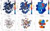 |
Fig. 5 H ii regions detection showing the application of the HIIexplorer software to NGC 628. The panels display the segmentation maps generated by the software. Left: original Z0 galaxies. Middle: Z1 galaxies. Right: Z2 galaxies. North is up, east is to the left. These segmentation maps are later used for the extraction of the H ii region spectra. |
We used the HIIexplorer software (Sánchez et al. 2012b) to segregate and perform the corresponding spectral extraction of all the H ii regions detected on each map. The HIIexplorer works assuming: (a) H ii regions are peaky/isolated structures with strong ionized gas emission clearly above the continuum level emission and the average ionized gas emission across the galaxy, and (b) H ii regions have a typical physical size of about a hundred or few hundreds of parsecs (e.g. González Delgado & Pérez 1997; López et al. 2011; Oey et al. 2003), which corresponds to a typical projected size of a few arcsec at the distance of the observed galaxies. The algorithm requires a line emission map, with the same world-coordinate system (WCS) and resolution as the input datacube (preferentially an Hα emission line map). HIIexplorer outputs a segmentation FITS file describing the pixels associated to each H ii region map that should be used for the extraction of the spectra. Each region will have a single spectrum generated by co-adding all the spectra indicated by the segmentation map. In Fig. 5 we can see, as an example, the case of NGC 628 in the three redshift regimes. The number of H ii regions detected in each regime immediately indicates the effect of resolution degradation, i.e. as we go to higher redshift we are considering as one region the contribution from all H ii regions smaller than the resolution element. Even in the Z0 case, the real physical size of an H ii region is below the spatial resolution: in all cases, when we refer to H ii regions we are in fact considering H ii complexes or aggregates. Table 3 shows the number of detected regions, with good enough signal-to-noise ratio (S/N) to perform the analysis, following the criteria from Sánchez et al. (2012b), for all the galaxies in the present study. For example, from 331 regions detected in NGC 1058, the Z2 regime identifies only 7. For the Z1 case, the average factor of under-detection is ~3, and the difference between Z1 and the Z2 regime ~5. Also, as the resolution becomes coarser, the difficulty in delimiting the H ii regions implies that we are combining both diffuse gas and H ii region emission. It is important to mention that this is always the case if one is considering spaxel-to-spaxel analysis instead of individual or aggregations of H ii regions. The latter is required to minimize the effect of contamination due to diffuse gas. If H ii regions cannot be segregated, it is not guaranteed that the dominant ionized emission is due to photoionization from young massive stars and therefore, analysis as the abundance derivations are not reliable. This is probably the case for the Z2 case where, due to the low number of pixels, it is difficult to identify peaky/isolated structures as required by the HIIexplorer. As will be shown later for the abundance determination, although for the Z2 case the conditions are not easily fulfilled, the comparison between the spaxel-spaxel and the HIIexplorer analysis indicates that the former has a greater misinterpreting possibility, even considering a S/N threshold. As already mentioned in Sánchez et al. (2012b), the spatial sampling and resolution of the data presented in this work is not optimal for the derivation of additive properties of individual H ii regions. Therefore these data are not optimal for the study of the Hα luminosity function or the characteristic optical extension of H ii regions, to mention just a couple of quantities. Although in every analysis of this kind one has to bear in mind that the measurements could correspond to an H ii region complex.
Number of H ii regions detected for each galaxy.
When we reach the higher redshift regime the situation gets more complicated. We are adding together regions belonging to very different galactic components, considering that we are not distinguishing disc, arms, and bulge, but, in any case, it will depend on the morphology of the studied galaxy.
To explore further the H ii region limits mentioned above, we identified all the regions from the higher resolution datacube that are detected as an individual region at lower resolution. In this way we can analyse the real source (or sources) of a particular measurement, and study how it is affected by the spatial binning. Figure 6 shows an example for NGC 628. The upper panel of this figure displays a histogram of the number of Z0 regions inside a Z1 one. This distribution indicates that, on average, each Z1 detected H ii region is built of 3 smaller Z0 regions. For the higher redshift case, each individual region is, in reality, an agglomerate of around 15 to 25 Z0 regions, while it is built by the contribution of ~4 Z1 regions. Table 4 summarises the distribution of the number of regions in terms of median and standard deviation for all the sample.
Distribution of number of regions corresponding to different regimes.
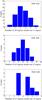 |
Fig. 6 Correspondence between the numbers of regions in each regime for NGC 628, i.e. the number of regions lying inside an individual region of each other redshift case. Upper panel: correspondence between Z0 and Z1. Middle panel: correspondence between Z0 and Z2. Lower panel: correspondence between Z1 and Z2. |
5.2.2. Diagnostic diagrams
We can use the [O iii]λ5007/Hβ ratio, together with [N ii]λ6583/ Hα, to construct the classical BPT diagram for all the galaxies, as shown in Fig. 7. These plots allow us to see how the spatial information loss is affecting our understanding and characterisation of the ionisation sources at higher redshift. It is clear that when the idea is to separate, for example, AGN activity from star-formation, one has to consider the degree of contamination due to the area subtended by the spectroscopic aperture. In the present study, where we are dealing with H ii regions, we have the opportunity to map the way that this resolution degradation alters the position of each individual region on the BPT diagram. We have also plotted the Kewley et al. (2001) demarcation curve, often invoked to distinguish between star-forming regions (Fig. 7, below the red line), and other sources of ionisation, such as AGN/shocks/post-AGB stars (above the line) and the Kauffmann et al. (2003) one to indicate the so-called composite zone. In the plots, empty circles correspond to the Z0 case, while full blue circles and orange squares correspond to Z1 and Z2 respectively. We also plot symbol size proportional to the galactocentric distance, i.e. the larger the symbol, the farther from the galaxy centre.
This distribution of regions in the BTP diagram is expected since star-formation is the dominant ionising source in all the selected galaxies. As described in Kewley & Ellison (2008) the objects lying in the composite region do not require an additional ionising source per se, in the case of a strong nitrogen enrichment. Other ionisation sources, like shocks, AGB star and AGN photoionization, mixed with pure star-formation, can also populate this region. Thus, the intermediate region only indicates that their nature is uncertain, not that the ionising source is definitely different than star-formation. However, for the particular scope of this article, we have preferred a conservative approach and do not consider them in any further discussion.
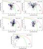 |
Fig. 7 Classical BPT emission-line diagnostic diagrams (Baldwin et al. 1981; Veilleux & Osterbrock 1987) with the demarcation curves of Kewley et al. (2001) (upper curve, red) and Kauffmann et al. (2003) (lower curve, green) for each galaxy. Empty circles correspond to Z0, blue circles to Z1, and orange squares to Z2. Symbol sizes are proportional to galactocentric distance, i.e. the larger symbols are, the farther from the centre. |
In the Z1 case of NGC 628 (blue circles), the effect of spatial resolution degradations is a collapse of the regions into the most populated zone of the Z0 plot (empty circles), and then again, for the Z2 regime, all regions are more concentrated in the “core” of the lower redshift case. In the Z2 case we do not see composite regions, with all lying in the star formation zone. The same behaviour is displayed in the BPT diagrams of the other galaxies, except for NGC 1637 with several Z2 points in the composite area. The BPT diagram of NGC 1058 displays the strongest collapse effect. Figure 8 shows the behaviour of one individual Z2 region of NGC 628 and its constituents from the other redshift regimes. The underlying reason of the shrinking in the occupied parameter space with increasing Z could be because the ratios are luminosity-weighted. If two regions have R1 = a1/b1 and R2 = a2/b2, then the combined ratio R = (a1 + a2)/b = R1 × (b1/b) + R2 × (b2/b), where b = b1 + b2. In the case where b1 ≫ b2(b1 ≪ b2), then R ~ R1(R2). When b1 ~ b2, then R ~ 0.5 × (R1 + R2). R is always between R1 and R2. Therefore, summing multiple H ii regions and measuring line ratios mean taking a luminosity-weighted mean of the ratios.
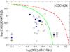 |
Fig. 8 Same as Fig.7 but for one Z2 region and its corresponding Z0 and Z1 region content. Empty circles correspond to Z0, blue circles to Z1, and orange squares to Z2. |
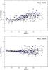 |
Fig. 9 Top: radial distribution of [O iii]/Hβ for NGC 1058. Bottom: radial distribution of the [N ii]/Hα ratio for the same galaxy. Empty circles correspond to Z0, blue circles to Z1, and orange squares to Z2. |
In all the Z1 simulated galaxies the approximate shape of the two-branches structure, visible in the original Z0 galaxies is acceptably discerned. Thus, we suggest that Z1 can recover the global trend of H ii regions in the BPT diagram while Z2 only reflects the denser part of the distribution in the lower redshift case.
5.2.3. Line ratios and abundances
For the derivation of the oxygen abundance we adopted the O3N2 indicator using the calibration provided by Pettini & Pagel (2004), defined by the relation 12 + log(OH) = 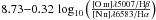 . This calibration has the advantage of being relatively easy to measure (based on strong emission lines), is basically not affected by the effects of extinction (the involved line-ratios are very close in wavelength), and implies a simple linear conversion, reason for which this indicator is very popular for high redshift studies3 Fig. 9 shows the radial distributions of the ratios [N ii]/Hα and [O iii]/Hβ. We can see that the [O iii]/Hβ radial gradient becomes flatter with redshift. This will have a clear effect on the abundance determination. As an example, Fig. 10 shows the radial abundances for regions in two of the galaxies (NGC 1058 and NGC 1637) with fitted gradients for comparison purposes, corresponding the empty circles to Z0, the blue circles to Z1, and the orange squares to Z2 (see Fig. A.1 for the remaining objects).
We note that the oxygen abundance is not an additive but a relative property, and it exhibits a ubiquitous radial gradient (e.g. Sánchez et al. 2012b). Therefore, neither the average nor a value at a fixed aperture are characteristic of the full distribution (e.g. Tremonti et al. 2004; Rosales-Ortega et al. 2012). Even more, it is still not clear that the average of the values derived at different radii is representative of a single value derived using an aperture that encircles all the previous ones.
In all the galaxies we see a radial abundance gradient decreasing outwards, with NGC 628 and NGC 1058 being the more evident cases. This effect is expected as late-type galaxies are known to have a composition gradient related to their star formation history (SFH). The capability of any survey of being able to measure this gradient is essential if one of its goals is to characterise the properties of galactic discs.
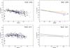 |
Fig. 10 Radial abundance gradients derived using the relation O3N2 from Pettini & Pagel (2004) for two of the galaxies. In each left panel the three redshift regimes are over-plotted, the empty circles correspond to Z0, the blue circles to Z1, and the orange squares to Z2. The three points in the bottom left corner show the average error bars. In the right panels we can see a linear regression fitting to each regime. |
All galaxies show a nearly flat distribution in the innermost parts, until r ~ 0.2R25. From this point, the abundance measurements start to exhibit higher values, reaching maxima at r ~ 0.4R25 in 3 of the cases (r ~ 0.2R25 for NGC 1058). After this, the slope of the radial abundance distribution changes its sign, and decreases with increasing galactocentric radius. In all cases, Z1 reproduces notably the Z0 trend with slightly lower abundances. The same radial gradients are visible, with the only difference being the absence of the peak at r ~ 0.2R25 (in the case of NGC 1058) and r ~ 0.4R25 (for NGC 628). For all the galaxies, Z2 fails to reproduce the slope behaviour, as anticipated with the [O iii]/Hβ line ratio, showing a nearly flatter distribution (on average) like in NGC 1058 and NGC 1637 (see Fig. 10).
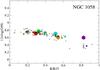 |
Fig. 11 Radial abundance gradient of NGC 1058 for the three redshift regimes. Colour coded is each different Z2 region with its corresponding Z0 and Z1 components (same colour). Small circles correspond to Z0, medium sized to Z1 and the bigger ones to Z2. Plus signs represent the abundance determined summing the flux of all the Z0 regions inside the corresponding Z2 region, while crosses are the determination from the total flux of Z1 regions (also the ones inside the Z2 region). |
Figure 10 shows that for the higher redshift simulation the abundance flattens. To search for possible sources of this behaviour on the radial abundance distribution for Z2, we performed several tests. We used the H ii regions catalogue of Sánchez et al. (2012b) to simulate a spatial binning adding together all the H ii regions inside different apertures. The observed effect was a simple average of the H ii region properties as expected, discarding the sum of H ii regions as source of the flattening. This can be also confirmed in Fig. 11 that shows the radial abundance gradient of NGC 1058 for the three redshift regimes. Colour coded is each different Z2 region with its corresponding Z0 and Z1 components (same colour). Small circles correspond to Z0, medium sized to Z1 and the bigger ones to Z2. Plus signs represent the abundance determined summing the flux of all the Z0 regions inside the corresponding Z2 region, while crosses are the determination from the total flux of the Z1 regions inside that Z2 region.
It is well known that the derivation of Balmer emission line fluxes are affected by the accuracy of the subtraction of the underlying stellar population. In particular, Hβ is strongly affected. Along the pilot studies for the CALIFA survey (Mármol-Queraltó et al. 2011), studied the capability of recovering this emission line at different equivalent widths, underlying stellar populations, and spectral resolutions. We noticed that at low equivalent widths Hβ is overestimated for old stellar populations and underestimated for young stellar populations. This effect is stronger at lower spectral resolutions. The net effect of the decrease in the spatial sampling produces these three combined effects: (i) it reduces the original equivalent width by increasing more regions dominated by low-intensity diffuse emission, increasing the underlying continuum with respect to the gas emission; (ii) it increases the fraction of old stellar populations in the inner regions, and the fraction of young stellar populations in the outer ones; and (iii) it decreases the effective spectral resolution by the beam effect, i.e. the co-adding of regions with different kinematic properties. All together it produces an increase in [O iii]/Hβ in the inner regions and its decrease in the outer ones. For galaxies with a positive gradient in [N ii]/Hα it produces a flattening of the radial abundance.
This effect is also present in other abundance indicators, like R23, and less affected by others like [N ii]/Hα. Evidently, the effect of the spatial resolution degradation on the Z2 regime inhibits any possibility of measuring convincing radial abundance gradients at that redshift.
Yuan et al. (2013) find similar results studying the [N ii]/Hα ratio. They show that seeing-limited observations produce significantly flatter gradients than higher angular resolution observations. They find a critical angular resolution FWHM range (<0.02″), which depends on the intrinsic gradient of the galaxy, beyond which the measured metallicity is significantly more flattened than the intrinsic metallicity.
Another effect that may be playing an important role on the radial abundance gradients and the BPT diagrams, is that when we go to higher redshift, the coarse resolution causes us to add more diffuse gaseous component to the H ii aggregates, with potentially different dominating ionising sources than in the H ii complexes. The difference between the plus sign, the cross and the bigger circles of Fig. 11 would account for the different amount of diffuse medium considered on each region. The effect of this contamination is very clear if we study cases where we can resolve the diffuse medium at tens-of-parsec scale like in M33 or NGC 5253 (e.g. Voges & Walterbos 2006; Relaño et al. 2010; Monreal-Ibero et al. 2010a, 2011). In all the mentioned cases, as we move away from the H ii region, with the maximum local Hα flux, as this flux decreases, the ratio [N ii]/Hα increases while [O iii]/Hβ decreases. This will cause the abundance determination based on the O3N2 method to increase. If in a considered galaxy the H ii region spatial density is low, the contribution of the diffuse component to the line ratios could become very important and even the dominant source of line fluxes, i.e. as could be the case in the outer points of the radial abundance distribution plotted in Fig. 10. In any case, an estimation of the contribution of the diffuse component is not trivial and depends on the different galaxy components considered (arm, inter-arm, bulge, nucleus, etc.).
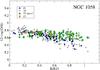 |
Fig. 12 Comparison between the same analysis as Fig. 10 and a spaxel-spaxel determination above a S/N threshold (green) for NGC 1058. |
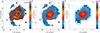 |
Fig. 13 Isophotal fit performed to V-band images extracted from the NGC 628 datacubes. Flux scale is in arbitrary units. For clarity, only some isophotes (black lines) are depicted on the plots. This fitting is later used as segmentation maps for the spectral extraction, i.e the extraction will be performed adding all the spectra between two isophotes separated by a given flux step. North is up, east is to the left. Left: Z0, centre: Z1, right:Z2. |
Figure 12 shows the comparison between the same analysis as Fig. 10 and an spaxel-spaxel determination above a S/N threshold. The low abundance inner pixels may alter the gradient determination. Although a deep analysis of the merging H ii complexes and the contribution from diffuse ionized gas (DIG) is beyond the scope of this paper, it is worth noting that they are key points in this kind of studies, and any interpretation should consider them. Although the DIG contribution to the integrated flux in some lines has been quantified in large values (e.g. about 30%–50% of ionized gas, as traced by Hα, in galaxies is found outside of H ii regions, Thilker et al. 2002; Oey et al. 2007; Haffner et al. 2009; Monreal-Ibero et al. 2010b; Alonso-Herrero et al. 2010), its final contribution to dust corrected luminosity is much lower (e.g. 5%–30%, Crocker et al. 2013; Sánchez et al. 2013). The line ratio of the DIG may differ from that of the star-forming regions, being in general located in the LINER-like region of the BTP diagram (Singh et al. 2013; Papaderos et al. 2013), reflecting ionizing conditions that depend on the morphology of the galaxies (e.g. post-AGBs for most of the earlier-type galaxies, Papaderos et al. 2013). Therefore, the inclusion of larger fraction of DIG emission as the resolution is degraded have a clear effect in the line ratios, although it is the not the only effect to take into account.
When the spatial resolution is good enough to resolve the more luminous H ii regions, it is still possible to use techniques of crowded field spectroscopy (Fabrika et al. 2005; Blanc et al. 2009; Kamann et al. 2013). These techniques are extensions to IFS of the well-known PSF-photometric techniques (DAOPhot), and they rely on the basis that the considered regions are basically unresolved at the spatial resolution of the data. Therefore, it is possible to perform a multi-Gaussian 2D fitting, wavelength by wavelength, to model each of the individual HII-regions, and a 2D polinomial function to take into account the continuum. This procedure will effectively decouple the diffuse from the resolved emission. However, for doing so it is required to distinguish between both components, and, as we argue along this article, this is not feasible with the spatial resolution of the Z2 data. We have still not implemented this procedure in HIIexplorer, but we will have to add that capability to perform more detailed analysis in the future.
It is clear that the effects in the line ratios and the corresponding derivation of the abundance gradients are complex, and involve many different components that are difficult to disentangle. However, the final result may produce a change in this gradient induced by the degradation of the resolution.
With all the considerations made above, the parameters studied for the gaseous phase show that, contrary to the naive picture, the effect of the resolution degradation is not as intuitive as it would be if we were considering simple additive quantities. Some effects detected in abundance gradients or BPT diagrams at high redshift could be due to spatial information loss.
5.3. Stellar component
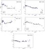 |
Fig. 14 Radial distribution of the D4000 index defined as the ratio of the flux in the red continuum to that in the blue continuum. Black empty circles correspond to Z0 regime, blue circles to Z1, and orange squares to Z2. The error bars are similar to the symbol sizes. |
As we explained in Sect. 5, we used FIT3D for separating the gaseous spectra from the underlying stellar population. In the previous sections we showed the analysis for the gaseous phase, and in what follows we are going to deal with the stellar component.
Spectral indices are widely used for the characterisation of stellar population in galaxies (Trager et al. 2000; Gallazzi et al. 2005). It is beyond the scope of this paper to analyse which method is most suitable for the detail study of stellar population. In the present study we chose the D4000 index to analyse how their derived properties vary in the different redshift regimes. D4000 is a good tracer of stellar age, besides being model-independent. Errors were determined running a Montecarlo simulation during the fitting procedure.
The chosen approach was to generate segmentation maps doing an isophotal fitting to the V-band images extracted from the datacubes. The basic idea of any binning for the analysis of data is to increase the S/N as much as possible while minimising the degradation of the spatial information. The most widely adopted binning procedure for the analysis of IFS data is the one described by Cappellari & Copin (2003). This technique performs a binning of the data intended to increase the S/N of the low-surface brightness areas, considering spatial vicinity. However, it does not take into account the morphology (relative intensity) between adjacent pixels, which is understandable since it was mostly adopted for the analysis of early-type galaxies (SAURON/ATLAS3D data). For the analysis of galaxies rich in structure (like the ones included in the current study), we consider that a more representative binning should take into account the relative intensity of adjacent pixels.
A similar effect is shown in the standard procedures to derive isophotal distribution of properties (e.g. surface-brightness profiles as the one described in Sect. 5.1). They well describe the azimuthal distribution of properties for early type galaxies, but they do not work as well for late type galaxies.
Therefore, we propose a more simple method to derive isophotal information similar to the one introduced by Papaderos et al. (2002). Instead of assuming a certain shape for the isophote at a certain radii, we just slice the intensity maps on bins of equal intensity, within a certain percentage. Starting from the peak emission of a galaxy, and selecting the range of adjacent pixels to be aggregated within a selected percentage of flux with respect to the peak emission, and iterating until reaching a certain surface brightness, it is possible to bin the data in isophotal areas without any assumption on their shape. Once segregated the galaxy in isophotal areas, it is possible to extract the corresponding co-added spectra, and analyse them. For a given isophotal bin, the distance considered is the distance from the galaxy centre to the average distance to each isophote. This technique provides azimuthal distributions of properties that describe better the actual shape of the galaxies.
If in addition to this simple criteria, a maximum distance between adjacent pixels is considered, then we will end-up with a 2D binning technique that preserves the actual shape of the galaxies. The details of the technique and its comparison with other methods will be described elsewhere.
In Fig. 13 we can see an example for this segmentation method for NGC 628. As described in detail in Sánchez et al. (2007), FIT3D measures the stellar indices from the extracted stellar spectra, normalised to the standard Lick/IDS resolution.
Figure 14 displays the radial distribution of the D4000 index for all of the sample. Being sensitive to stellar age, this index is higher in the presence of an older stellar population.
For all the galaxies, the Z0 radial behaviour of the D4000 index (open circles) is totally reproduced by the Z1 regime (blue circles). Only the innermost regions, when a sharp structure is present, it is slightly smeared out in the Z1 case. The higher redshift regime (orange squares) follows the radial trend when the distribution is smooth, as is the case of NGC 1058. Z2 is unable to reproduce the innermost structures presented in NGC 628, NGC 3184 and NGC 1637.
All these indices are luminosity weighted. Summing two spaxels means performing a luminosity-weighted average of their D4000 break strength, so the observed behaviour is more intuitive than the one for the more complex emission line ratios. Unlike the gaseous phase where we have the information in clumps, the stellar component contains the information in a smooth, less clumpy way. In the cases where the radial D4000 distribution is flatter, the spatial resolution loss has a small effect at higher redshifts. This behaviour allows the higher redshift regime to follow the radial trend without much scatter, although loosing any fine detail present in the distribution.
We conducted similar test with other stellar indices as Hδ index, i.e. the equivalent width of the Balmer line Hδ, and the [MgFe] index (![Mathematical equation: \hbox{$\textnormal{[MgFe]} = \sqrt{ \textnormal{Mg}b\, (0.72\, \textnormal{Fe}_{5270} + 0.28\, \textnormal{Fe}_{5335})}$}](/articles/aa/full_html/2014/01/aa21789-13/aa21789-13-eq102.png) ). As a result of our low spectral resolution we are not able to confirm if complex indices based on absorption lines (as [MgFe]) are traceable to higher redshift, but we can conclude that simple ones like Hδ or D4000 are.
). As a result of our low spectral resolution we are not able to confirm if complex indices based on absorption lines (as [MgFe]) are traceable to higher redshift, but we can conclude that simple ones like Hδ or D4000 are.
6. Summary and conclusions
In this paper we have studied how the information loss due to spatial resolution degradation would affect IFS surveys at different redshifts. For this purpose we used a sample of five PINGS galaxies (Z0) and simulated two redshift regimes without taking into account surface brightness dimming or increase in noise. One associated with the ongoing CALIFA survey (Z1) and the other with an hypothetical higher redshift survey (Z2). We then performed the same analysis to the Z0 galaxies and their simulated versions. We studied the behaviour of the radial abundance (through the O3N2 method), BPT diagrams, and one spectral index D4000, in addition to the Hα emission and the morphology. Our main conclusions regarding each measured quantity, can be summarised as follows:
-
Morphology: Z1 is able to reproduce all morphological signatures visible at lower redshift. Despite the detail loss (implying that several individual regions or hot spots are not detected as such), spiral arms, rings and bulge extensions can be traced perfectly. For the Z2 regime the identification of spiral signatures is complicated, and only possible if the structure is a strong morphological feature on a global scale in the galaxy. Several of the higher redshift examples shown in this paper present disturbed morphology that prevents from doing a reliable morphological classification.
-
H ii regions detection: the implemented method of H ii region detection with HIIexplorer, showed that Z1 is detecting nearly 1/3 of the number of original Z0 regions, and Z2 ~ 1/5 of the number of regions detected at the Z1 redshift (hence, ~1/15 of Z0). This illustrates what is the underestimation of the number of H ii regions due the loss of spatial resolution.
-
Diagnostic diagrams: the BPT diagrams showed that the effect of spatial resolution degradation on this diagrams is to collapse the measured values into the denser regions of Z0 plots. Z1 is able to reproduce with acceptable accuracy the shape of the Z0 BPT. For the Z2 situation, only the most populated regions of the lower redshift regime are mapped. Despite the displacement observed, the main ionization mechanism of the observed galaxy at the putative higher redshift is mostly due to thermal ionization from hot massive young stars.
-
Radial abundance: The O3N2 method (commonly used at high redshift to derive gas metallicity) was applied to our sample. It showed that the flat inner part of the abundance distribution presented in the Z0 galaxies is observable in the Z1 case and, although with smoothed values, in Z2. Z1 and Z2 are able to reproduce the maximum value displayed around (0.2 − 0.4)R25 in the Z0 galaxies. The gradient slopes in Z0 are slightly smoothed in Z1 but still present. In the higher redshift case global trends are traceable. We note that the degradation and contamination of H ii complexes at higher redshift may induce spurious radial trends.
-
Spectral indices: for the analysed index D4000, global tendencies are correctly traced on both simulated cases, and Z1 is also capable, at some level, of reproducing fine structure of the Z0 distributions.
As a global conclusion, we showed that the information loss will depend on the level of detail contained in the analysed feature. In this sense, if the studied galaxy has a smooth profile, early-type, with smooth behaviour in their properties, that behaviour will still be visible at higher redshift. But any sharp structure will be lost. Our analysis allows us to conclude that CALIFA will be able to analyse to an acceptable scale, and with a good level of detail, all desired magnitudes, in its aim of characterising the Local Universe. For the hypothetical higher redshift survey, the perspectives are difficult but promising, since global trends, averaged values, and, in some cases, local structures, are acceptably mapped and correctly interpreted in the considered framework.
It is worth noting that the important figure of merit is the ratio between the spaxel size and the typical scale-length at a certain redshift. As examples of hypothetical Z2 surveys, we can consider SAMI (1.6′′/fibre) or MaNGA (3′′/fibre). In this regard, the conclusions obtained for the Z2 simulation are also applicable to other redshift ranges depending on the instrument. For example, if we are studying galaxies with ~0.25 kpc/spaxel, we have shown that most of the common observables are perfectly traced, while this is not the case with a scale of 1 ~kpc/spaxel.
As real examples, we can consider the Gemini Multi-Object Spectrographs (GMOS; Allington-Smith et al. 2002). With 25 × 35 spaxels and a 0.2′′/spaxel scale our results showed that at z ~ 0.05 it is still possible to derive radial gradients, whenever the right depth and spatial coverage are granted. The same conclusion can be applied to VIMOS (VIsible MultiObject Spectrograph, Le Fèvre et al. 2003) in the Medium Resolution mode (a 13″ × 13″ FoV with 0.33′′/spaxel). But, as we have already shown, at z ~ 0.4, for example, none of these instruments is capable of measuring properly any of the observables studied. Another positive example could be SINFONI (Spectrograph for INtegral Field Observations in the Near Infrared, Eisenhauer et al. 2003) in its 8″ × 8″ FoV with a 0.125″ × 0.125″ spaxel, or even with the 3″ × 3″ mode, provided that the Adaptive Optics Facility is used, z ~ 0.1 can be reached with considerable success. In the usual redshift ranges that SINFONI has been used (z ~ 1), we have shown that no convincing metallicity radial gradients can be obtained with the data.
IRAF is distributed by the National Optical Astronomy Observatories, which are operated by the Association of Universities for Research in Astronomy, Inc., under cooperative agreement with the National Science Foundation.
This indicator has been recently re-calibrated for the high-metallicity regime by Marino et al. (2013). Although there is a known discrepancy in deriving metallicity with different calibrators (Kewley & Ellison 2008), Sánchez et al. (2012b) showed that there is a correlation between the different determinations, the discrepancies present at high redshift being, to a large degree, a consequence of resolution effects. In any case, although the specific results obtained here are applicable to the O3N2 calibrator in particular, the use of one or the other calibration does not modify qualitatively the results of the proposed analysis. Other methods will suffer from different systematic effects (e.g. absolute scale differences), which analysis are beyond the scope of this paper.
Acknowledgments
We would like to thank the anonymous referee for his/her useful comments that have significantly improved the first submitted version of this paper. Based on observations collected at the Centro Astronómico Hispano-Alemán (CAHA) at Calar Alto, operated jointly by the Max-Planck Institut für Astronomie and the Instituto de Astrofísica de Andalucía (CSIC). D.M. and A.M.-I. are supported by the Spanish Research Council within the programme JAE-Doc, Junta para la Ampliación de Estudios, co-funded by the FSE. F.F.R.O. acknowledges financial support from the Mexican National Council for Science and Technology (CONACYT) under the programme Estancias Posdoctorales y Sabáticas al Extranjero para la Consolidación de Grupos de Investigación, 2010-2012. I.M. acknowledges financial support from the Spanish MINECO grant AYA 2010-15169, and from Junta de Andalucía TIC114 and Proyecto de Excelencia P08-TIC-03531; J.F.-B. from the Ramón y Cajal Program, grants AYA2010-21322-C03-02 and AIB-2010-DE-00227 from the Spanish Ministry of Economy and Competitiveness (MINECO), as well as from the FP7 Marie Curie Actions of the European Commission, via the Initial Training Network DAGAL under REA grant agreement na¸289313. C.J.W. acknowledges support through the Marie Curie Career Integration Grant 303912. E.M.Q. and J.F.-B. acknowledge support from the Spanish Programa Nacional de Astronomía y Astrofísica under grant AYA2010-21322-C03-02. This work has been partially funded by the Spanish PNAYA, project AYA2010-21887 of the Spanish MINECO. R.A. Marino was also funded by the Spanish Programme of International Campus of Excellence Moncloa (CEI).
References
- Allington-Smith, J., Murray, G., Content, R., et al. 2002, PASP, 114, 892 [NASA ADS] [CrossRef] [Google Scholar]
- Alonso-Herrero, A., García-Marín, M., Rodríguez Zaurín, J., et al. 2010, A&A, 522, A7 [NASA ADS] [CrossRef] [EDP Sciences] [Google Scholar]
- Baldwin, J. A., Phillips, M. M., & Terlevich, R. 1981, PASP, 93, 5 [NASA ADS] [CrossRef] [EDP Sciences] [Google Scholar]
- Balogh, M. L., Morris, S. L., Yee, H. K. C., Carlberg, R. G., & Ellingson, E. 1999, ApJ, 527, 54 [NASA ADS] [CrossRef] [Google Scholar]
- Barden, M., Jahnke, K., & Häumlußler, B. 2008, ApJS, 175, 105 [NASA ADS] [CrossRef] [MathSciNet] [Google Scholar]
- Bennett, C. L., Halpern, M., Hinshaw, G., et al. 2003, ApJS, 148, 1 [NASA ADS] [CrossRef] [Google Scholar]
- Bershady, M. A., Verheijen, M. A. W., Swaters, R. A., et al. 2010, ApJ, 716, 198 [NASA ADS] [CrossRef] [Google Scholar]
- Blanc, G. A., Heiderman, A., Gebhardt, K., Evans, N. J., II, & Adams, J. 2009, ApJ, 704, 842 [NASA ADS] [CrossRef] [Google Scholar]
- Blanc, G. A., Gebhardt, K., Heiderman, A., et al. 2010, New Horizons in Astronomy: Frank N. Bash Symposium 2009, ASP Conf. Ser., 432, 180 [NASA ADS] [Google Scholar]
- Caon, N., Capaccioli, M., D’Onofrio, M., & Longo, G. 1994, A&A, 286, L39 [NASA ADS] [Google Scholar]
- Cappellari, M., & Copin, Y. 2003, MNRAS, 342, 345 [NASA ADS] [CrossRef] [Google Scholar]
- Cappellari, M., Emsellem, E., Krajnović, D., et al. 2011, MNRAS, 413, 813 [NASA ADS] [CrossRef] [Google Scholar]
- Cardelli, J. A., Clayton, G. C., & Mathis, J. S. 1989, ApJ, 345, 245 [NASA ADS] [CrossRef] [Google Scholar]
- Casoli, F., Combes, F., Dupraz, C., Gerin, M., & Boulanger, F. 1986, A&A, 169, 281 [NASA ADS] [Google Scholar]
- Crocker, A. F., Calzetti, D., Thilker, D. A., et al. 2013, ApJ, 762, 79 [NASA ADS] [CrossRef] [Google Scholar]
- Croom, S. M., Lawrence, J. S., Bland-Hawthorn, J., et al. 2012, MNRAS, 421, 872 [NASA ADS] [Google Scholar]
- de Vaucouleurs, G., de Vaucouleurs, A., Corwin, H. G., Jr., et al. 1992, VizieR Online Data Catalog: VII/137B [Google Scholar]
- de Zeeuw, P. T., Bureau, M., Emsellem, E., et al. 2002, MNRAS, 329, 513 [NASA ADS] [CrossRef] [Google Scholar]
- Dutil, Y., & Roy, J.-R. 1999, ApJ, 516, 62 [NASA ADS] [CrossRef] [Google Scholar]
- Eisenhauer, F., Abuter, R., Bickert, K., et al. 2003, Proc. SPIE, 4841, 1548 [Google Scholar]
- Fabrika, S., Sholukhova, O., Becker, T., et al. 2005, A&A, 437, 217 [NASA ADS] [CrossRef] [EDP Sciences] [Google Scholar]
- Förster Schreiber, N. M. 2009, in Proc. Unveiling the Mass Extracting and Interpreting Galaxy Masses, id.44 [Google Scholar]
- Gallazzi, A., Charlot, S., Brinchmann, J., White, S. D. M., & Tremonti, C. A. 2005, MNRAS, 362, 41 [NASA ADS] [CrossRef] [Google Scholar]
- García-Benito, R., Pérez, E., Díaz, Á. I., Maíz Apellániz, J., & Cerviño, M. 2011, AJ, 141, 126 [NASA ADS] [CrossRef] [Google Scholar]
- Garnett, D. R., & Shields, G. A. 1987, ApJ, 317, 82 [NASA ADS] [CrossRef] [Google Scholar]
- Garnett, D. R., Shields, G. A., Skillman, E. D., Sagan, S. P., & Dufour, R. J. 1997, ApJ, 489, 63 [NASA ADS] [CrossRef] [Google Scholar]
- Genzel, R., Lutz, D., Sturm, E., et al. 1998, ApJ, 498, 579 [NASA ADS] [CrossRef] [Google Scholar]
- Giavalisco, M., Livio, M., Bohlin, R. C., Macchetto, F. D., & Stecher, T. P. 1996, AJ, 112, 369 [NASA ADS] [CrossRef] [Google Scholar]
- González Delgado, R. M., & Pérez, E. 1997, ApJS, 108, 199 [NASA ADS] [CrossRef] [Google Scholar]
- Graham, A. W., Driver, S. P., Petrosian, V., et al. 2005, AJ, 130, 1535 [NASA ADS] [CrossRef] [Google Scholar]
- Graham, A. W., Merritt, D., Moore, B., Diemand, J., & Terzić, B. 2006, AJ, 132, 2711 [NASA ADS] [CrossRef] [Google Scholar]
- Haffner, L. M., Dettmar, R.-J., Beckman, J. E., et al. 2009, Rev. Mod. Phys., 81, 969 [NASA ADS] [CrossRef] [Google Scholar]
- Hendry, M. A., Smartt, S. J., Maund, J. R., et al. 2005, MNRAS, 359, 906 [NASA ADS] [CrossRef] [Google Scholar]
- Jones, T., Ellis, R., Jullo, E., & Richard, J. 2010, ApJ, 725, L176 [NASA ADS] [CrossRef] [Google Scholar]
- Kamann, S., Wisotzki, L., & Roth, M. M. 2013, A&A, 549, A71 [NASA ADS] [CrossRef] [EDP Sciences] [Google Scholar]
- Kauffmann, G., Heckman, T. M., Tremonti, C., et al. 2003, MNRAS, 346, 1055 [Google Scholar]
- Kelz, A., & Roth, M. M. 2006, New A Rev., 50, 355 [Google Scholar]
- Kelz, A., Verheijen, M. A. W., Roth, M. M., et al. 2006, PASP, 118, 129 [NASA ADS] [CrossRef] [Google Scholar]
- Kennicutt, R. C., Jr. 1998, ARA&A, 36, 189 [Google Scholar]
- Kennicutt, R. C., Jr., & Garnett, D. R. 1996, ApJ, 456, 504 [NASA ADS] [CrossRef] [Google Scholar]
- Kewley, L. J., & Ellison, S. L. 2008, ApJ, 681, 1183 [NASA ADS] [CrossRef] [Google Scholar]
- Kewley, L. J., Dopita, M. A., Sutherland, R. S., Heisler, C. A., & Trevena, J. 2001, ApJ, 556, 121 [Google Scholar]
- Kewley, L. J., Groves, B., Kauffmann, G., & Heckman, T. 2006, MNRAS, 372, 961 [NASA ADS] [CrossRef] [Google Scholar]
- Kormendy, J. 1977, ApJ, 218, 333 [NASA ADS] [CrossRef] [Google Scholar]
- Kronberger, T., Kapferer, W., Schindler, S., & Ziegler, B. L. 2007, A&A, 473, 761 [Google Scholar]
- Law, D. R., Steidel, C. C., & Erb, D. K. 2006, AJ, 131, 70 [NASA ADS] [CrossRef] [Google Scholar]
- LeFèvre, O., Saisse, M., Mancini, D., et al. 2003, Proc. SPIE, 4841, 1670 [NASA ADS] [CrossRef] [Google Scholar]
- López, L. A., Krumholz, M. R., Bolatto, A. D., Prochaska, J. X., & Ramirez-Ruiz, E. 2011, ApJ, 731, 91 [NASA ADS] [CrossRef] [Google Scholar]
- Marino, R. A., Rosales-Ortega, F. F., Sánchez, S. F., et al. 2013, A&A, 559, A114 [NASA ADS] [CrossRef] [EDP Sciences] [Google Scholar]
- Mármol-Queraltó, E., Sánchez, S. F., Marino, R. A., et al. 2011, A&A, 534, A8 [NASA ADS] [CrossRef] [EDP Sciences] [Google Scholar]
- Monreal-Ibero, A., Vílchez, J. M., Walsh, J. R., & Muñoz-Tuñón, C. 2010a, A&A, 517, A27 [NASA ADS] [CrossRef] [EDP Sciences] [Google Scholar]
- Monreal-Ibero, A., Arribas, S., Colina, L., et al. 2010b, A&A, 517, A28 [NASA ADS] [CrossRef] [EDP Sciences] [Google Scholar]
- Monreal-Ibero, A., Relaño, M., Kehrig, C., et al. 2011, MNRAS, 413, 2242 [NASA ADS] [CrossRef] [Google Scholar]
- Moustakas, J., Kennicutt, R. C., Jr., Tremonti, C. A., et al. 2010, ApJS, 190, 233 [NASA ADS] [CrossRef] [Google Scholar]
- Oey, M. S., Parker, J. S., Mikles, V. J., & Zhang, X. 2003, AJ, 126, 2317 [NASA ADS] [CrossRef] [Google Scholar]
- Oey, M. S., Meurer, G. R., Yelda, S., et al. 2007, ApJ, 661, 801 [NASA ADS] [CrossRef] [Google Scholar]
- Papaderos, P., Izotov, Y. I., Thuan, T. X., et al. 2002, A&A, 393, 461 [NASA ADS] [CrossRef] [EDP Sciences] [Google Scholar]
- Papaderos, P., Gomes, J. M., Vílchez, J. M., et al. 2013, A&A, 555, L1 [NASA ADS] [CrossRef] [EDP Sciences] [Google Scholar]
- Pettini, M., & Pagel, B. E. J. 2004, MNRAS, 348, L59 [NASA ADS] [CrossRef] [Google Scholar]
- Pilyugin, L. S., Vílchez, J. M., & Contini, T. 2004, A&A, 425, 849 [NASA ADS] [CrossRef] [EDP Sciences] [Google Scholar]
- Queyrel, J., Contini, T., Kissler-Patig, M., et al. 2012, A&A, 539, A93 [NASA ADS] [CrossRef] [EDP Sciences] [Google Scholar]
- Ravikumar, C. D., Puech, M., Flores, H., et al. 2007, A&A, 465, 1099 [NASA ADS] [CrossRef] [EDP Sciences] [Google Scholar]
- Relaño, M., Monreal-Ibero, A., Vílchez, J. M., & Kennicutt, R. C. 2010, MNRAS, 402, 1635 [NASA ADS] [CrossRef] [Google Scholar]
- Rodríguez Zaurín, J., Tadhunter, C. N., & González Delgado, R. M. 2008, MNRAS, 384, 875 [NASA ADS] [CrossRef] [Google Scholar]
- Rosales-Ortega, F. F., Kennicutt, R. C., Sánchez, S. F., et al. 2010, MNRAS, 405, 735 [NASA ADS] [Google Scholar]
- Rosales-Ortega, F. F., Díaz, A. I., Kennicutt, R. C., & Sánchez, S. F. 2011, MNRAS, 415, 2439 [NASA ADS] [CrossRef] [Google Scholar]
- Rosales-Ortega, F. F., Sánchez, S. F., Iglesias-Páramo, J., et al. 2012, ApJ, 756, L31 [NASA ADS] [CrossRef] [Google Scholar]
- Rosolowsky, E., & Simon, J. D. 2008, ApJ, 675, 1213 [NASA ADS] [CrossRef] [Google Scholar]
- Roth, M. M., Kelz, A., Fechner, T., et al. 2005, PASP, 117, 620 [NASA ADS] [CrossRef] [Google Scholar]
- Sánchez, S. F. 2004, Astron. Nachr., 325, 167 [NASA ADS] [CrossRef] [Google Scholar]
- Sánchez, S. F. 2006, Astron. Nachr., 327, 850 [NASA ADS] [CrossRef] [Google Scholar]
- Sánchez, S. F., Cardiel, N., Verheijen, M. A. W., Pedraz, S., & Covone, G. 2007, MNRAS, 376, 125 [NASA ADS] [CrossRef] [Google Scholar]
- Sánchez, S. F., Rosales-Ortega, F. F., Kennicutt, R. C., et al. 2011, MNRAS, 410, 313 [NASA ADS] [CrossRef] [Google Scholar]
- Sánchez, S. F., Kennicutt, R. C., Gil de Paz, A., et al. 2012a, A&A, 538, A8 [NASA ADS] [CrossRef] [EDP Sciences] [Google Scholar]
- Sánchez, S. F., Rosales-Ortega, F. F., Marino, R. A., et al. 2012b, A&A, 546, A2 [NASA ADS] [CrossRef] [EDP Sciences] [Google Scholar]
- Sánchez, S. F., Rosales-Ortega, F. F., Jungwiert, B., et al. 2013, A&A, 554, A58 [NASA ADS] [CrossRef] [EDP Sciences] [Google Scholar]
- Sánchez-Portal, M., Cepa, J., Pintos-Castro, I., et al. 2011, in Highlights of Spanish Astrophysics VI, eds. M. R. Zapatero Osorio, J. Gorgas, J. Maíz Apellániz, J. R. Pardo, & A. Gil de Paz, Proc. IX Scientific Meeting of the EAS, 353 [Google Scholar]
- Schawinski, K., Thomas, D., Sarzi, M., et al. 2007, MNRAS, 382, 1415 [NASA ADS] [CrossRef] [Google Scholar]
- Shaver, P. A., McGee, R. X., Newton, L. M., Danks, A. C., & Pottasch, S. R. 1983, MNRAS, 204, 53 [NASA ADS] [CrossRef] [Google Scholar]
- Singh, R., van de Ven, G., Jahnke, K., et al. 2013, A&A, 558, A43 [NASA ADS] [CrossRef] [EDP Sciences] [Google Scholar]
- Swinbank, M., Sobral, D., Smail, I., et al. 2012, MNRAS, submitted [arXiv:1209.1395] [Google Scholar]
- Taylor, M. B. 2005, Astronomical Data Analysis Software and Systems XIV, eds. P. Shopbell, M. Britton, & R. Ebert, ASP Conf. Ser., 347, 29 [Google Scholar]
- Thilker, D. A., Walterbos, R. A. M., Braun, R., & Hoopes, C. G. 2002, AJ, 124, 3118 [NASA ADS] [CrossRef] [Google Scholar]
- Trager, S. C., Faber, S. M., Worthey, G., & González, J. J. 2000, AJ, 120, 165 [NASA ADS] [CrossRef] [Google Scholar]
- Tremonti, C. A., Heckman, T. M., Kauffmann, G., et al. 2004, ApJ, 613, 898 [NASA ADS] [CrossRef] [Google Scholar]
- van Zee, L., Salzer, J. J., Haynes, M. P., O’Donoghue, A. A., & Balonek, T. J. 1998, AJ, 116, 2805 [NASA ADS] [CrossRef] [Google Scholar]
- Vazdekis, A., Sánchez-Blázquez, P., Falcón-Barroso, J., et al. 2010, MNRAS, 404, 1639 [NASA ADS] [Google Scholar]
- Veilleux, S., & Osterbrock, D. E. 1987, ApJS, 63, 295 [NASA ADS] [CrossRef] [Google Scholar]
- Vergani, D., Epinat, B., Contini, T., et al. 2012, A&A, 546, A118 [NASA ADS] [CrossRef] [EDP Sciences] [Google Scholar]
- Verheijen, M. A. W., Bershady, M. A., Andersen, D. R., et al. 2004, Astron. Nachr., 325, 151 [NASA ADS] [CrossRef] [Google Scholar]
- Viironen, K., Sánchez, S. F., Marmol-Queraltó, E., et al. 2012, A&A, 538, A144 [NASA ADS] [CrossRef] [EDP Sciences] [Google Scholar]
- Vila-Costas, M. B., & Edmunds, M. G. 1992, MNRAS, 259, 121 [NASA ADS] [CrossRef] [Google Scholar]
- Voges, E. S., & Walterbos, R. A. M. 2006, ApJ, 644, L29 [NASA ADS] [CrossRef] [Google Scholar]
- Webster, B. L., & Smith, M. G. 1983, MNRAS, 204, 743 [NASA ADS] [Google Scholar]
- Yuan, T.-T., Kewley, L. J., & Rich, J. 2013, ApJ, 767, 106 [NASA ADS] [CrossRef] [Google Scholar]
- Zaritsky, D., Kennicutt, R. C., Jr., & Huchra, J. P. 1994, ApJ, 420, 87 [NASA ADS] [CrossRef] [Google Scholar]
Appendix A: Radial abundance determination for the remaining objects
In Sect. 5.2.3, for presentation purposes, we showed only two objects. In Fig. A.1 the radial abundance gradients for the remaining galaxies are shown.
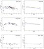 |
Fig. A.1 Radial abundance gradients derived using the relation O3N2 from Pettini & Pagel (2004) for the three remaining galaxies. In each left panel the three redshift regimes are over-plotted, the empty circles correspond to Z0, the blue circles to Z1, and the orange squares to Z2. The three points in the lower left corner (upper left for NGC 5474) show the average error bars. In the right panels we can see a linear regression fitting to each regime. |
Appendix B: Annular binning
One binning scheme widely used in different surveys and metallicity studies is the annular binning extraction, method which is often used to derive metallicity gradients, specially in low S/N high-z data (e.g., Jones et al. 2010; Queyrel et al. 2012; Swinbank et al. 2012; Yuan et al. 2013). Figure B.1 shows the radial abundance gradients for all the sample, using this binning method. Annuli are one pixel wide for all the redshift regimes. The black line overplotted on the graph represents the abundance determination of Sect. 5.2.3 for the Z0 regime using the HIIexplorer. As this method wipe out any azimuthal variation and add together the H ii region and the diffuse emission (that in general do no have the same ionizing conditions as the starforming-regions) for a given annulus on all the three regimes, the result is not surprising. Radial distributions have low dispersion compared with the ones in Sect. 5.2.3 and small scale variations are smeared out as resolution gets coarse.
As can be seen from the plots, in the cases where the DIG is not dominated by LINER-like emission, the radial distribution for the three regimes are more similar (despite the small variations), indicating that for these cases the use of the annular binning extraction scheme would be more suitable at higher redshift. In any case it will depend on the morphology and distribution of the HII regions on each particular galaxy, information that in general is not available for high-redshift objects.
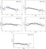 |
Fig. B.1 Radial abundance gradients for all the sample, using the annular binning scheme for the spectral extraction. On each redshift regime annuli are one pixel wide (on its corresponding scale). In each panel the three redshift regimes are over-plotted, the empty circles correspond to Z0, the blue circles to Z1, and the orange squares to Z2 as usual. The black line indicates the Z0 abundance gradient determined in Sect. 5.2.3. |
All Tables
All Figures
|
Fig. 1 Digital Sky Survey R-band images of the five galaxies selected from PINGS for this study (adapted from RO10). The IFS mosaicking is indicated by the superposition of the hexagonal PPak FoVs. Images are 10 × 10 arcmin2. North is up, east is to the left. |
| In the text | |
|
Fig. 2 V-band images constructed from the datacubes. Flux scale in arbitrary units. Left: original PINGS galaxies. Middle: Z1 galaxies. Right: Z2 galaxies. North is up, east is to the left. |
| In the text | |
|
Fig. 2 continued. |
| In the text | |
|
Fig. 3 Surface brightness profiles of the original PINGS galaxies and the simulated ones, constructed fitting ellipses to V-band images extracted from the datacubes. The profiles were scaled in the y-axis to make them coincide at Rmax/2 (maximum measured radius divided by 2). |
| In the text | |
|
Fig. 4 Hα images extracted from the cubes. Flux is in units of 10-16 erg s-1 cm-2 Å-1. Z1 and Z2 are scaled to Z0 flux. Left: original Z0 galaxies. Middle: Z1 galaxies. Right: Z2 galaxies. North is up, east is to the left. The Hα map of NGC 628 is displayed in Fig. 5. |
| In the text | |
|
Fig. 5 H ii regions detection showing the application of the HIIexplorer software to NGC 628. The panels display the segmentation maps generated by the software. Left: original Z0 galaxies. Middle: Z1 galaxies. Right: Z2 galaxies. North is up, east is to the left. These segmentation maps are later used for the extraction of the H ii region spectra. |
| In the text | |
|
Fig. 6 Correspondence between the numbers of regions in each regime for NGC 628, i.e. the number of regions lying inside an individual region of each other redshift case. Upper panel: correspondence between Z0 and Z1. Middle panel: correspondence between Z0 and Z2. Lower panel: correspondence between Z1 and Z2. |
| In the text | |
|
Fig. 7 Classical BPT emission-line diagnostic diagrams (Baldwin et al. 1981; Veilleux & Osterbrock 1987) with the demarcation curves of Kewley et al. (2001) (upper curve, red) and Kauffmann et al. (2003) (lower curve, green) for each galaxy. Empty circles correspond to Z0, blue circles to Z1, and orange squares to Z2. Symbol sizes are proportional to galactocentric distance, i.e. the larger symbols are, the farther from the centre. |
| In the text | |
|
Fig. 8 Same as Fig.7 but for one Z2 region and its corresponding Z0 and Z1 region content. Empty circles correspond to Z0, blue circles to Z1, and orange squares to Z2. |
| In the text | |
|
Fig. 9 Top: radial distribution of [O iii]/Hβ for NGC 1058. Bottom: radial distribution of the [N ii]/Hα ratio for the same galaxy. Empty circles correspond to Z0, blue circles to Z1, and orange squares to Z2. |
| In the text | |
|
Fig. 10 Radial abundance gradients derived using the relation O3N2 from Pettini & Pagel (2004) for two of the galaxies. In each left panel the three redshift regimes are over-plotted, the empty circles correspond to Z0, the blue circles to Z1, and the orange squares to Z2. The three points in the bottom left corner show the average error bars. In the right panels we can see a linear regression fitting to each regime. |
| In the text | |
|
Fig. 11 Radial abundance gradient of NGC 1058 for the three redshift regimes. Colour coded is each different Z2 region with its corresponding Z0 and Z1 components (same colour). Small circles correspond to Z0, medium sized to Z1 and the bigger ones to Z2. Plus signs represent the abundance determined summing the flux of all the Z0 regions inside the corresponding Z2 region, while crosses are the determination from the total flux of Z1 regions (also the ones inside the Z2 region). |
| In the text | |
|
Fig. 12 Comparison between the same analysis as Fig. 10 and a spaxel-spaxel determination above a S/N threshold (green) for NGC 1058. |
| In the text | |
|
Fig. 13 Isophotal fit performed to V-band images extracted from the NGC 628 datacubes. Flux scale is in arbitrary units. For clarity, only some isophotes (black lines) are depicted on the plots. This fitting is later used as segmentation maps for the spectral extraction, i.e the extraction will be performed adding all the spectra between two isophotes separated by a given flux step. North is up, east is to the left. Left: Z0, centre: Z1, right:Z2. |
| In the text | |
|
Fig. 14 Radial distribution of the D4000 index defined as the ratio of the flux in the red continuum to that in the blue continuum. Black empty circles correspond to Z0 regime, blue circles to Z1, and orange squares to Z2. The error bars are similar to the symbol sizes. |
| In the text | |
|
Fig. A.1 Radial abundance gradients derived using the relation O3N2 from Pettini & Pagel (2004) for the three remaining galaxies. In each left panel the three redshift regimes are over-plotted, the empty circles correspond to Z0, the blue circles to Z1, and the orange squares to Z2. The three points in the lower left corner (upper left for NGC 5474) show the average error bars. In the right panels we can see a linear regression fitting to each regime. |
| In the text | |
|
Fig. B.1 Radial abundance gradients for all the sample, using the annular binning scheme for the spectral extraction. On each redshift regime annuli are one pixel wide (on its corresponding scale). In each panel the three redshift regimes are over-plotted, the empty circles correspond to Z0, the blue circles to Z1, and the orange squares to Z2 as usual. The black line indicates the Z0 abundance gradient determined in Sect. 5.2.3. |
| In the text | |
Current usage metrics show cumulative count of Article Views (full-text article views including HTML views, PDF and ePub downloads, according to the available data) and Abstracts Views on Vision4Press platform.
Data correspond to usage on the plateform after 2015. The current usage metrics is available 48-96 hours after online publication and is updated daily on week days.
Initial download of the metrics may take a while.