| Issue |
A&A
Volume 559, November 2013
|
|
|---|---|---|
| Article Number | A82 | |
| Number of page(s) | 8 | |
| Section | Interstellar and circumstellar matter | |
| DOI | https://doi.org/10.1051/0004-6361/201322463 | |
| Published online | 18 November 2013 | |
Interplay between chemistry and dynamics in embedded protostellar disks⋆
1 Niels Bohr Institute, University of Copenhagen, Juliane Maries Vej 30, 2100 Copenhagen Ø, Denmark
e-mail:
This email address is being protected from spambots. You need JavaScript enabled to view it.
2 Centre for Star and Planet Formation and Natural History Museum of Denmark, University of Copenhagen, Øster Voldgade 5–7, 1350 Copenhagen K., Denmark
Received: 8 August 2013
Accepted: 25 September 2013
Abstract
Context. A fundamental part of the study of star formation is to place young stellar objects in an evolutionary sequence. Establishing a robust evolutionary classification scheme allows us not only to understand how the Sun was born but also to predict what kind of main sequence star a given protostar will become. Traditionally, low-mass young stellar objects are classified according to the shape of their spectral energy distributions. Such methods are, however, prone to misclassification due to degeneracy and do not constrain the temporal evolution. More recently, young stellar objects have been classified based on envelope, disk, and stellar masses determined from resolved images of their continuum and line emission at submillimeter wavelengths.
Aims. Through detailed modeling of two Class I sources, we aim at determining accurate velocity profiles and explore the role of freeze-out chemistry in such objects.
Methods. We present new Submillimeter Array observations of the continuum and HCO+ line emission at 1.1 mm toward two protostars, IRS 63 and IRS 43 in the Ophiuchus star forming region. The sources were modeled in detail using dust radiation transfer to fit the SED and continuum images and line radiation transfer to produce synthetic position-velocity diagrams. We used a χ2 search algorithm to find the best model fit to the data and to estimate the errors in the model variables.
Results. Our best fit models present disk, envelope, and stellar masses, as well as the HCO+ abundance and inclination of both sources. We also identify a ring structure with a radius of about 200 AU in IRS 63.
Conclusions. We find that freeze-out chemistry is important in IRS 63 but not for IRS 43. We show that the velocity field in IRS 43 is consistent with Keplerian rotation. Owing to molecular depletion, it is not possible to draw a similar conclusion for IRS 63. We identify a ring-shaped structure in IRS 63 on the same spatial scale as the disk outer radius. No such structure is seen in IRS 43.
Key words: stars: formation / stars: pre-main sequence / circumstellar matter / radiative transfer / submillimeter: stars
Reduced data cubes are only available at the CDS via anonymous ftp to cdsarc.u-strasbg.fr (130.79.128.5) or via http://cdsarc.u-strasbg.fr/viz-bin/qcat?J/A+A/559/A82
© ESO, 2013
1. Introduction
Gas dynamics is an all-important diagnostic tool in the field of star formation. It is governed by the gravitational pull from the newly formed star, as well as by the conservation of the angular momentum carried by the gas itself. Spectroscopic observations of the gas surrounding young stars tell us about the current accretion rate, the amount of turbulence, the presence and importance of outflows, and even the evolutionary stage of young stellar objects: in the earliest protostellar stages gas will predominantly move along radial trajectories as the cloud collapses but will eventually settle down in Keplerian orbits in the newly formed disk. To derive meaningful information from spectroscopic observations, it is important to understand the distribution of molecules, that is, the chemistry. Chemical depletion, whether due to freeze-out, dissociation, or gas-phase reactions, can mask important dynamical regions, such as the disk, and thus hide the signatures of accretion or rotation. On the other hand, if the depletion can be accurately determined from detailed modeling of the gas dynamics, we can get valuable information on the chemistry as a function of time (e.g., review by Bergin et al. 2007).
Protostellar evolution is often described by a series of distinct evolutionary pictures associated with the classification scheme of Lada & Wilking (1984), Lada (1987), and André et al. (1993). In reality, the evolution is a smooth, continuous process where the protostellar envelope is being accreted while the star and the protoplanetary disk grow. It is mostly agreed that the classes 0, I, II, and III represent a monotonous time progression (e.g., Evans et al. 2009). There is, however, currently no consensus about how sources of a single class can be sorted with respect to their absolute age. Attempts have been made (e.g., Myers & Ladd 1993) to introduce a continuous parametrization of protostellar evolution, usually based on properties of the spectral energy distribution (SED).
Robitaille et al. (2006) recognized that all the various classifications that are based on the spectral index do not necessarily distinguish between objects that are physically, hence evolutionarily distinct. For example, the same source can be classified differently depending on the viewing angle. They introduced an analogous classification scheme, where classes are denoted “Stage”, which is based on physical properties, such as mass and accretion rate. The main difficulty of classifying stars based on physical properties is that a modeling effort is always, to some extent, required, which is both time consuming and labor intensive as opposed to classifications that are based on apparent properties (such as the shape of the SED) which are easily automated.
Jørgensen et al. (2009) observed a sample of Class 0 and I sources and looked for evolutionary tracers based on observable properties such as envelope mass derived from the single dish (low resolution) submillimeter flux, disk mass derived from the high-resolution compact flux, and stellar luminosity derived from the SED. One conclusion of this study was that the disk mass does not change with decreasing envelope mass, that is, it is constant throughout the Class 0 and Class I stages. The question is however, how robust these derived values are compared to the ones obtained through detailed radiative transfer modeling of the data. Such modeling is non-trivial, however. A model should provide a description of the H2 density, the gas- and dust temperature, the molecular abundance, and the velocity field that need to be constrained by multi-wavelength line and continuum observations. Thanks to space missions like the Spitzer Space Telescope, ISO, and Herschel Space Observatory, as well as ground-based sub-millimeter continuum surveys large databases of young stars are becoming available. In addition, near-future observations with the Atacama Large Millimeter/submillimeter Array (ALMA) will provide a high degree of detail on individual sources.
In this paper, we present an extended analysis of two Class I protostellar sources in the Ophiuchus star-forming region1, IRS 43 and IRS 63, from the sample of Jørgensen et al. (2009). These two sources were chosen because they appear to be at a similar evolutionary stage. Nevertheless, they also show peculiar differences, namely that IRS 63 has weak HCO+ lines on top of a strong continuum while IRS 43 has strong lines on top of a weak continuum. We present additional high-angular resolution spectral line observations in the sub-millimeter and interpret these in the context of a detailed continuum and line radiative transfer model to asses their dynamical and chemical structure. Finally we discuss the exactness of simpler, more generic observations, with a particular eye on the perspectives opened-up by near-future ALMA observations.
2. Data
Observations of IRS 43 (IRAS 16244-2434) and IRS 63 (IRAS 16285-2355) were made using the Submillimeter Array (SMA, Ho et al. 2004)2 in extended configuration in July 2008 as a follow-up project to the PROSAC campaign (Jørgensen et al. 2007, 2009). Both sources were observed during a single track using all 8 telescopes, providing projected baselines between 16 kλ and 171 kλ. We used the same spectral set-up as was used in the original compact configuration track, namely one chunk of 512 channels centered on the HCO+J = 3–2 line (267.557648 GHz) providing a spectral resolution of 0.23 km s-1. Another high-resolution chunk was placed over the HCN J =3–2 line, but this line is undetected for both sources in the extended configuration track. The remaining bandwidth was used to measure the continuum at 1.1 millimeter. All calibration and data reduction were done in IDL using the MIR package (Qi 2007) and the data were combined with the compact configuration data using MIRIAD (Sault et al. 1995). The combined datasets have synthesized beams of 1.2′′ × 1.1′′ and 1.7′′ × 1.4′′ for IRS 63 and IRS 43, respectively. For IRS 63, the RMS noise is 2.9 mJy beam-1 for the continuum and 0.2 Jy beam-1 channel-1 for the HCO+ line. For IRS 43, the RMS for the continuum and the HCO+ line is 1.7 mJy beam-1 and 0.2 Jy beam-1 channel-1.
In this paper we also make use of archival data of both sources. These data include images from the SCUBA legacy catalogues (Di Francesco et al. 2008), the 2MASS survey (Skrutskie et al. 2006), a Spitzer/IRS spectrum of IRS 63 from the c2d legacy project (Evans et al. 2003), J, H, and K band photometry of IRS 43 (Haisch et al. 2002), as well as 1.1 mm fluxes from CSO/Bolocam survey (Young et al. 2006). In addition, we use a 55–200 μm PACS spectrum of IRS 63 from the Herschel Space Observatory DIGIT key program (Green et al. 2013).
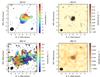 |
Fig. 1 Moment 0 (contour) and 1 (color) maps of the HCO+J = 3 − 2 line (left) and 1.1 mm continuum image (right) of IRS 63 and IRS 43. The beam is shown by the black ellipses. The dashed grey line marks the direction of the velocity gradient. |
3. Results
Figure 1 shows reconstructed images of the HCO+ line and the continuum emission as observed by the SMA. Natural weighting of the visibilities was used for the reconstruction in both cases. While the continuum is seen to be only marginally resolved, the HCO+ is well resolved for both sources. The line is considerably brighter in IRS 43 than in IRS 63 and vice versa for the continuum. Both sources show a clear velocity gradient.
The structure of IRS 63 was studied by Lommen et al. (2008) who used the PROSAC compact configuration data from the SMA to derive disk and envelope masses. The compact configuration data have projected baselines up to 60 kλ corresponding to a linear scale of about 440 AU. The disk is unresolved and therefore only the disk mass is constrained on these scales. In our extended configuration data with baselines of 171 kλ (linear scales of 150 AU) the disk is resolved, however. Figure 2 shows the visibility amplitudes of the continuum at 1.1 mm, with the symbols in green showing the visibilities covered by the compact configuration data and symbols in blue showing the visibilities covered by the extended configuration data. The extended configuration data suggest the presence of a face-on ring structure with an approximate diameter of 2.9′′ equivalent to a linear radius of 180 AU at the distance of IRS 63. Figure 2 also shows the Fourier transform of such a ring (with an arbitrary flux) plotted in red. The data obviously also contain the signal from the other components of circumstellar material and therefore the vertical offset of the red curve is not meant as a fit to the data but only as a guide to the eye. The fact that the nulls appear sharper in the data than in our Fourier transformed ring is due the fact that we use an infinitely thin (1D) ring whereas in reality the ring is probably a bit extended and with fuzzy edges. The extended configuration continuum amplitudes of IRS 43, which has a much weaker continuum signature than IRS 63, do not show a similar ring pattern, implying either that either no such structure exists in IRS 43 or, more likely, that the disk in IRS 43 is oriented in such a way that this structure, whatever it may be, is not seen as a ring.
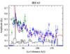 |
Fig. 2 Continuum visibility amplitudes of IRS 63 at 1.1 mm. The green markers are the visibilites covered by the PROSAC compact configuration track while the blue markers show the data covered by the extended configuration track. The black histogram shows the zero-signal expectation. The red curve shows the Fourier transform of a thin ring with a radius of 180 AU. |
4. Modeling
4.1. The continuum
In order to proceed, physical models of our two sources are needed. Although a physical model of IRS63 was presented by Lommen et al. (2008), we have chosen to redo the modeling for two reasons. First of all, we have much more data to constrain the model. Secondly, the data were fit-by-eye by Lommen et al. (2008), whereas we are able to do a systematic search of the parameter space and provide error bars on our best fit parameter values. As mentioned above, we use a simple three component model to describe the two YSOs, a protostar, a disk, and an envelope. The star is described by its surface temperature and the stellar radius, which together give its total luminosity. We use the standard description of a 2D disk in hydrostatic equilibrium parameterized by 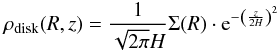 (1)where,
  We fix H0 = 40 AU, leaving us with two free parameters for the disk, the surface density Σ0 at R0 and the outer radius where the density profile (Eq. (1)) is truncated. The inner radius of the disk has been fixed at 1 AU. This choice may to some extent affect the appearance of the SED at near-infrared wavelengths, but this has no influence on the parameter values we derive in this paper. We did not include the disk inclination as a free parameter, but rather adopted a value for IRS 63 of 30° from Lommen et al. (2008) who based that number on the brightness of the 3−5 μm fluxes. Note also that in order to see the ring structure in the visibility amplitudes as described in Sect. 3, the disk needs to be relatively face-on. We did however test SEDs calculated for both higher and lower inclinations and found that while any fit is largely indistinguishable at inclinations lower than 30°, the fits become rapidly worse at inclinations higher than 50°. We did not have a previous estimate for the inclination for IRS 43, but we adopted a high inclination of 70° based on the flattened appearance of the HCO+ moment map (Fig. 1) and the fact that we do not see any sign of a ring pattern in the continuum visibility amplitudes.
For the envelope we use a simple spherical power-law model,  (4)with four free parameters, the density ρ0 at R0, the power-law slope p, and the inner and outer radius of the envelope. The total density is given by the sum of ρdisk and ρenv.
With these profiles we have eight free parameters in total. The temperature is calculated self-consistently using the radiation transfer code RADMC-3D3 and opacities of coagulated dust with thin ice mantles from Ossenkopf & Henning (1994). We use the LIME radiation transfer code (Brinch & Hogerheijde 2010) to calculate continuum images at 450 μm and 850 μm, and 1.1 mm. The latter is sampled by the visibilities from our SMA observations and (u,v)-amplitudes are extracted from the resulting visibility set using MIRIAD. The model fluxes from RADMC-3D and the images and visibilities from LIME are compared simultaneously to the SED, the SCUBA images and the SMA 1.1 mm visibility amplitudes. The eight input parameters are varied to obtain the best fitting model. We use the PIKAIA genetic algorithm (Charbonneau 1995) to search the parameter space and once the best fit has been found, a local gradient search algorithm is used to estimate the error bars on the parameter values. We assume that the errors in the data are dominated by a 20% calibration uncertainty. We ran more than hundred thousand SED models for the PIKAIA algorithm to converge on the best solution and we ran the optimization scheme twice to make sure that the same solution was obtained using a different random number seed. The error bars on the parameter values are determined by the distance along the axis in parameter space where the χ2 value has increased by one with respect to the best fit χ2 value.
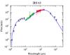 |
Fig. 3 SED of IRS 63 with the best fit model shown with a blue line. Each flux point is shown with a 20% calibration error bar. The green spectrum is from the Spitzer Space Telescope and the red spectrum is from the Herschel Space Observatory. The near-infrared points are observations from 2MASS and Spitzer/IRAC. The submillimeter data points are from SCUBA (450 μm and 850 μm) and CSO (1.1 mm). |
First we consider IRS 63. Including the Spitzer IRS and Herschel PACS spectra for IRS 63, we have a fully sampled SED from 10 to 200 μm. The resulting best SED fit is shown in Fig. 3 and the corresponding best fits to the SCUBA and SMA data are shown in Fig. 4. The comparison between our model and the SMA data is done in (u,v)-space: after multiplication with the primary beam of the SMA and Fourier transformation, the model is sampled with the observed visibilities. Table 1 shows the best fit parameters for IRS 63, including error bars. The disk surface density and envelope reference density are given at the disk radius and the outer radius of the envelope respectively. Interestingly, we find a best fitting disk radius of 165 AU which is almost the same radius as the ring we identified in the continuum visibilities in Sect. 3, even though we binned the visibilities in much wider bins to smooth out the nulls during the model optimization.
Best fit continuum model parameters and 1σ error bars (for IRS 63).
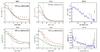 |
Fig. 4 Continuum model of IRS 63 (top row) and IRS 43 (bottom row). The panels show from left to right the model fit to the radial brightness distribution of the SCUBA images and the model fit to the 1.1 mm SMA averaged visibility amplitudes. In the SCUBA profile plots, the data are shown with a red histogram and the model with a green histogram. The black dashed curve is a 2D Gaussian fit to the data. The vertical dashed line indicates the beam size. The visibility amplitudes of IRS 63 are the same as are shown in Fig. 2 but binned in much wider bins. In the visibility plots, the Fourier transform of the model is shown in blue. |
For IRS 43, there is neither a Spitzer nor a Herschel spectrum. The SED of IRS 43 is therefore rather sparse, with only a single MIPS 70 μm flux point to constrain the mid-infrared part. Correspondingly, PIKAIA could not find a unique solution. The SEDs of IRS 63 and IRS 43, however, are very similar in shape. Therefore, we chose to adopt the same model that fits IRS 63 and simply do a small adjustment to the luminosity and envelope mass to accommodate the difference in absolute flux and then fine tune the resulting solution with a gradient search algorithm to find the local minimum. The best fits to the SED and to the sub-millimeter data can be seen in Figs. 4 and 5, respectively, and the corresponding parameter values are given in Table 1. The solution works surprisingly well, suggesting that the two sources are indeed very similar in nature. The main discrepancy between data and the model is at 850 μm where the peak flux is off by a factor of two. As can be seen in the 850 μm SCUBA image, however, the emission is contaminated by a neighboring source offset by 35′′ and therefore the 20% error bar on the 850 μm flux point on the SED is probably much too small. Because of the lack of a unique solution for IRS 43, we do not give error bars on the parameter values.
4.2. The spectral lines
Once the physical models of IRS 63 and IRS 43 are constrained by continuum emission, we model the HCO+J = 3–2 emission lines. At first, we assume a constant abundance for HCO+ which only requires one additional free parameter. The velocity model that we use is the one first introduced by Brinch et al. (2007a). This model assumes an average velocity field that is spanned by a linear combination of pure free infall and pure Keplerian rotation. The two free parameters are the central (stellar) mass and the ratio of the two basis vectors or rather the angle of the resulting velocity vectors with respect to the azimuthal direction, 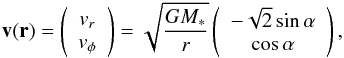 (5)where α is the angle between v(r) and the unit vector
  .
.
We pass the physical model including this velocity field to the molecular excitation and radiation transfer code LIME, which creates synthetic spectral image cubes. These are post-processed with MIRIAD to construct synthetic observations that can be compared directly to our SMA data. We used collision rates between HCO+ and H2 from Flower (1999) taken from the LAMDA database (Schöier et al. 2005). We also fix the turbulent line broadening at 200 m s-1. Again we run the optimization scheme but here constrain the parameters based on the PV-diagrams. We evaluate our fit in (u,v)-space rather than in the image plane. We thus construct the equivalent to an ordinary PV-diagram directly from the (u,v)-data by fitting a Gaussian to the (u,v)-flux on a channel-by-channel basis. The centroid of these Gaussians form a one-dimensional PV-diagram as can be seen in Fig. 6 a) and b) where they are plotted as black crosses on top of the contoured PV-diagram extracted from the image plane. The distribution of emission is reasonably well reproduced, but in the case of IRS 43, we miss some of the high-velocity emission in the wings of the central spectrum at ±6−7 km s-1, which could be due to a small contribution of high-velocity outflow.
Panels c) and d) in Fig. 6 show our best fit models and the red curves show the best fit radial velocity distribution. The parameters of the fit are given in Table 2. While the velocity model for IRS 43 fits the data almost perfectly, the model for IRS 63 overproduces the velocities between offsets of ± 1 − 3′′. This difference could indicate that we over-estimate either the central mass or the inclination. Lowering either the mass or the inclination makes the lines too narrow and single peaked (the data clearly show a double peak toward the central position), and therefore our best fit in the case of IRS 63 is a trade-off between reproducing the correct line shape and fitting the radial velocity profile. It should be noted that Lommen et al. (2008) find a stellar mass for IRS 63 which is about half of our value. Using their value makes our model consistent with the emission peak points seen in panel a) of Fig. 6, but the emission distribution is inconsistent.
A constant HCO+ abundance with respect to H2 fits the data well for both sources. The value, however, differs by almost a factor of 10 between the two sources. This difference can be explained by freeze-out of the molecules at low temperatures, particularly in the disk mid-plane and in the outer envelope. New models where the molecules are allowed to freeze-out by lowering the abundance by a factor of 10 at temperatures below 30 K produces an equally good fit to the PV-diagrams with an adjustment to the gas phase abundance. We find that while IRS 43 is hardly affected by the freeze-out and thus requires the same gas-phase abundance of 0.9 × 10⁻⁹ with respect to H2, the gas-phase abundance in IRS 63 needs to be adjusted by a large factor to make the model fit. It turns out that with a freeze out temperature of 30 K, IRS 63 needs to have exactly the same gas phase abundance as IRS 43. The explanation for this difference between the two sources is that the more massive disk in IRS 63 is much colder that the disk in IRS 43, and thus many more molecules are frozen out.
Best fit line model parameters for IRS 63 and IRS 43.
Comparison of sources.
Table 3 shows properties derived from our best fit models. We also include the corresponding properties of Taurus Class I source L1489 IRS for comparison (Brinch et al. 2007b).
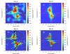 |
Fig. 6 PV-diagrams of a) IRS 63 and b) IRS 43 and the corresponding best fit models c) and d). The black points and error bars in a) and b) are the channel-by-channel Gaussian fit to the (u,v)-flux. The red curves are not Keplerian rotation, but rather the best fit velocity field as given by Eq. (5). The PV-diagrams a) and b) are taken along the grey line shown in Fig. 1. |
5. Discussion
We find that IRS 43 and IRS 63 are physically very similar to each other, in terms of their SEDs and their velocity fields. The peculiar difference in the relative strengths of the lines to the continuum is explained by geometry as well as a difference in the disk mass. The difference in disk mass as well as in luminosity explains why IRS 63 is more affected by freeze-out and if these differences are taken into account, the HCO+ abundances are indeed similar. This is likely a consequence of CO freeze-out on dust grains and consequently a drop in HCO+ as this species follows that of CO closely in protostars (Jørgensen 2004).
Various attempts in the recent literature have been made to measure the CO snow line using ALMA (Mathews et al. 2013; Qi et al. 2013). Given ALMA resolution, observations of HCO+ in IRS 63 could possibly also reveal the location of the CO snow line in this early disk. Figure 7 shows our best fit model of IRS 63 with and without freeze-out below 30 K in a high ALMA resolution of 0.05′′. While we do not see any distinguishable difference in the PV-diagrams between the freeze-out and no freeze-out cases with the resolution of the SMA (except for the absolute line intensity), there is a clear and distinguishable difference between the two cases when we go to a resolution of 0.05′′, at least when the freeze-out temperature is 30 K. For a freeze-out temperature of 20 K, the depleted region is too small to have any impact on the overall emission.
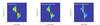 |
Fig. 7 PV-diagrams of the IRS 63 model in a high spatial resolution of 0.05′′. In the left panel, the HCO+ abundance is constant and in the center and the right panel, the HCO+ abundance is an order of magnitude lower at temperatures below 20 K and 30 K respectively. |
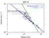 |
Fig. 8 Emission peaks per velocity channel from the PV-diagram of IRS 43 in panel b of Fig. 6, plotted in logarithmic space. The blue line shows our best fit velocity model and the green line shows the best r-1 profile that fits the data. |
We find that our best fit model parameters are close to the values derived in Jørgensen et al. (2009). Our model results on IRS 63 are also mostly consistent with the parameters derived by Lommen et al. (2008) except for the stellar mass. They, however, base their stellar mass on the PV-diagram alone (and with much sparser data) which, as discussed above, may lead to an inaccurate stellar mass. We thus conclude that envelope and disk masses and stellar luminosities of Class I sources can be safely derived directly from observations by measuring the total and the compact submillimeter flux and integrating the SED, as done by Jørgensen et al. (2009).
Currently, there is some discussion in the literature on whether Class I disks are truly Keplerian or whether the velocity field in these disks are consistent with other profiles too (Belloche 2013; Yen et al. 2013). As illustrated in Fig. 8, the velocity field of IRS 43, is in almost perfect agreement with a Keplerian r-0.5 profile. For comparison, we have also plotted the best possible r-1 profile which does not agree at all with the data. If we consider the IRS 63 velocity data in the same way, we get a much less clear picture. It is in fact possible to fit both profiles with about the same χ2. This indeterminacy, however, does not mean that IRS 63 does not have a Keplerian disk but is simply a reflection of the fact that an almost face-on disk shows very weak rotation signature and that the signal-to-noise ratios of the IRS 63 line are not high. From a purely geometrical argument, about 15% of all disks have an inclination of 30° (like IRS 63) or lower, which means that at least 15% of all Class I objects with Keplerian disks may not show a strong, unique Keplerian velocity profile.
Figure 7 shows that freeze-out has the effect of removing emission from larger angular offsets. Figure 8 shows that it is exactly that emission which constrains the velocity profile and makes us able to distinguish Keplerian rotation from a r-1 velocity profile. It is therefore possible to mistake a r-0.5 profile for an r-1 profile in a Class I object, if one is using a tracer which is depleted, no matter the spatial resolution.
While the two sources appear rather similar, it is clear that IRS 63 has a more massive disk and less envelope left than IRS 43. This difference could be interpreted as one being more evolved that than the other. Both sources, however, only have about 10% mass left in the envelope and both are dominated by Keplerian rotation which means that they must both be close to the T Tauri stage. Although some very high-velocity material is seen in the spectrum of IRS 43, neither source shows any substantial outflow.
6. Summary
In this paper we present new high-angular resolution observations of HCO+J = 3−2 and the continuum at 1.1 mm of two Class I sources in Ophiuchus, IRS 63 and IRS 43. We perform detailed radiative transfer modeling of the dust in order to reproduce the SED as well as continuum images at 450 μm, 850 μm, and 1.1 mm. We go on to model the HCO+ line using a non-LTE radiative transfer method. We draw a number of conclusions based on this modeling:
-
We have identified a ring structure in the 1.1 mmcontinuum visibilities of IRS 63. No suchstructure is seen in IRS 43 and we conclude that thisdifference is due to the difference in inclination. The ringcoincides with the modeled disk radius, but our model fails toreproduce the signature in the (u,v)-plane. The ring does not appear in the image plane and the nature and origin of it is still an open question. Higher resolution and sensitivity observations with ALMA can potentially reveal the nature of this curious structure around the edge of the disk.
-
We show that the velocity field of IRS 43 is very well described by a Keplerian velocity field on scales between 10 and 700 AU. The case for Keplerian motion is not equally clear for IRS 63, due to the lack of signal-to-noise, but this is consistent with the fact that IRS 63 is seen more or less face-on whereas IRS 43 is much closer to edge-on.
-
We find that our best-fit model parameters are consistent with the results of previous studies, except for the case of the central mass of IRS 63, which we find was previously underestimated. We furthermore find that the freeze-out chemistry is important for IRS 63 and relatively unimportant for IRS 43 – likely a consequence of the more massive disk and less luminous central source of IRS 63 as compared to IRS 43. Table 3 shows that IRS 43 and IRS 63 are very similar to L1489 IRS, which has previously been claimed to be a unique source (Hogerheijde 2001). In particular, IRS 43 seems almost identical, especially when comparing their morphologies.
In this paper we adopt a distance of 125 pc to Ophiuchus (de Geus et al. 1989) to be consistent with previous work.
The Submillimeter Array is a joint project between the Smithsonian Astrophysical Observatory and the Academia Sinica Institute of Astronomy and Astrophysics, and is funded by the Smithsonian Institution and the Academia Sinica.
Acknowledgments
This research was supported by a grant from the Carlsberg Foundation to Christian Brinch, and by a grant from the Lundbeck Foundation Group Leader Fellowship and a grant from the Instrumentcenter for Danish Astrophysics (IDA) to Jes Jørgensen. Research at Centre for Star and Planet Formation is funded by the Danish National Research Foundation and the University of Copenhagen’s programme of excellence.
References
- André, P., Ward-Thompson, D., & Barsony, M. 1993, ApJ, 406, 122 [NASA ADS] [CrossRef] [Google Scholar]
- Belloche, A. 2013, EAS PS, 62, 25 [Google Scholar]
- Bergin, E. A., Aikawa, Y., Blake, G. A., & van Dishoeck, E. F. 2007, Protostars and Planets V, 751 [Google Scholar]
- Brinch, C., & Hogerheijde, M. R. 2010, A&A, 523, A25 [NASA ADS] [CrossRef] [EDP Sciences] [Google Scholar]
- Brinch, C., Crapsi, A., Hogerheijde, M. R., & Jørgensen, J. K. 2007a, A&A, 461, 1037 [NASA ADS] [CrossRef] [EDP Sciences] [Google Scholar]
- Brinch, C., Crapsi, A., Jørgensen, J. K., Hogerheijde, M. R., & Hill, T. 2007b, A&A, 475, 915 [Google Scholar]
- Charbonneau, P. 1995, ApJS, 101, 309 [NASA ADS] [CrossRef] [Google Scholar]
- de Geus, E. J., de Zeeuw, P. T., & Lub, J. 1989, A&A, 216, 44 [NASA ADS] [Google Scholar]
- Di Francesco, J., Johnstone, D., Kirk, H., MacKenzie, T., & Ledwosinska, E. 2008, ApJS, 175, 277 [NASA ADS] [CrossRef] [Google Scholar]
- Evans, N. J. I., Allen, L. E., Blake, G. A., et al. 2003, PASP, 115, 965 [NASA ADS] [CrossRef] [Google Scholar]
- Evans, N. J., Dunham, M. M., Jørgensen, J. K., et al. 2009, ApJS, 181, 321 [NASA ADS] [CrossRef] [Google Scholar]
- Flower, D. R. 1999, MNRAS, 305, 651 [NASA ADS] [CrossRef] [Google Scholar]
- Green, J. D., Evans, N. J. I., Jørgensen, J. K., et al. 2013, ApJ, 770, 123 [NASA ADS] [CrossRef] [Google Scholar]
- Haisch, K. E., Barsony, M., Greene, T. P., & Ressler, M. E. 2002, AJ, 124, 2841 [NASA ADS] [CrossRef] [Google Scholar]
- Ho, P. T. P., Moran, J. M., & Lo, K. Y. 2004, ApJ, 616, L1 [NASA ADS] [CrossRef] [Google Scholar]
- Hogerheijde, M. R. 2001, ApJ, 553, 618 [NASA ADS] [CrossRef] [Google Scholar]
- Jørgensen, J. K. 2004, A&A, 424, 589 [NASA ADS] [CrossRef] [EDP Sciences] [Google Scholar]
- Jørgensen, J. K., Bourke, T. L., Myers, P. C., et al. 2007, ApJ, 659, 479 [NASA ADS] [CrossRef] [Google Scholar]
- Jørgensen, J. K., van Dishoeck, E. F., Visser, R., et al. 2009, A&A, 507, 861 [NASA ADS] [CrossRef] [EDP Sciences] [Google Scholar]
- Lada, C. J. 1987, in Star forming regions; Proc. Symp., Sreward Observatory, Tucson, AZ, 1 [Google Scholar]
- Lada, C. J., & Wilking, B. A. 1984, ApJ, 287, 610 [NASA ADS] [CrossRef] [Google Scholar]
- Lommen, D., Jørgensen, J. K., van Dishoeck, E. F., & Crapsi, A. 2008, A&A, 481, 141 [NASA ADS] [CrossRef] [EDP Sciences] [Google Scholar]
- Mathews, G. S., Klaassen, P. D., Juhasz, A., et al. 2013, A&A, 557, A132 [NASA ADS] [CrossRef] [EDP Sciences] [Google Scholar]
- Myers, P. C., & Ladd, E. F. 1993, ApJ, 413, L47 [NASA ADS] [CrossRef] [Google Scholar]
- Ossenkopf, V., & Henning, T. 1994, A&A, 291, 943 [NASA ADS] [Google Scholar]
- Qi, C. 2007, The MIR cookbook, https://www.cfa.harvard.edu/cqi/mircook.html [Google Scholar]
- Qi, C., Oberg, K. I., Wilner, D. J., et al. 2013, Science, 341, 630 [NASA ADS] [CrossRef] [PubMed] [Google Scholar]
- Robitaille, T. P., Whitney, B. A., Indebetouw, R., Wood, K., & Denzmore, P. 2006, ApJS, 167, 256 [NASA ADS] [CrossRef] [Google Scholar]
- Sault, R. J., Teuben, P. J., & Wright, M. C. H. 1995, Astronomical Data Analysis Software and Systems IV, eds. R. A. show, H. E. Payne, & J. J. E. Hayes, ASP Conf. Ser., 77, 433 [Google Scholar]
- Schöier, F. L., van der Tak, F. F. S., van Dishoeck, E. F., & Black, J. H. 2005, A&A, 432, 369 [NASA ADS] [CrossRef] [EDP Sciences] [Google Scholar]
- Skrutskie, M. F., Cutri, R. M., Stiening, R., et al. 2006, AJ, 131, 1163 [NASA ADS] [CrossRef] [Google Scholar]
- Yen, H.-W., Takakuwa, S., Ohashi, N., & Ho, P. T. P. 2013, ApJ, 772, 22 [NASA ADS] [CrossRef] [Google Scholar]
- Young, K. E., Enoch, M. L., Evans, N. J. I., et al. 2006, ApJ, 644, 326 [NASA ADS] [CrossRef] [Google Scholar]
All Tables
All Figures
|
Fig. 1 Moment 0 (contour) and 1 (color) maps of the HCO+J = 3 − 2 line (left) and 1.1 mm continuum image (right) of IRS 63 and IRS 43. The beam is shown by the black ellipses. The dashed grey line marks the direction of the velocity gradient. |
| In the text | |
|
Fig. 2 Continuum visibility amplitudes of IRS 63 at 1.1 mm. The green markers are the visibilites covered by the PROSAC compact configuration track while the blue markers show the data covered by the extended configuration track. The black histogram shows the zero-signal expectation. The red curve shows the Fourier transform of a thin ring with a radius of 180 AU. |
| In the text | |
|
Fig. 3 SED of IRS 63 with the best fit model shown with a blue line. Each flux point is shown with a 20% calibration error bar. The green spectrum is from the Spitzer Space Telescope and the red spectrum is from the Herschel Space Observatory. The near-infrared points are observations from 2MASS and Spitzer/IRAC. The submillimeter data points are from SCUBA (450 μm and 850 μm) and CSO (1.1 mm). |
| In the text | |
|
Fig. 4 Continuum model of IRS 63 (top row) and IRS 43 (bottom row). The panels show from left to right the model fit to the radial brightness distribution of the SCUBA images and the model fit to the 1.1 mm SMA averaged visibility amplitudes. In the SCUBA profile plots, the data are shown with a red histogram and the model with a green histogram. The black dashed curve is a 2D Gaussian fit to the data. The vertical dashed line indicates the beam size. The visibility amplitudes of IRS 63 are the same as are shown in Fig. 2 but binned in much wider bins. In the visibility plots, the Fourier transform of the model is shown in blue. |
| In the text | |
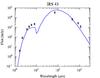 |
Fig. 5 Same as Fig. 3 but for IRS 43. |
| In the text | |
|
Fig. 6 PV-diagrams of a) IRS 63 and b) IRS 43 and the corresponding best fit models c) and d). The black points and error bars in a) and b) are the channel-by-channel Gaussian fit to the (u,v)-flux. The red curves are not Keplerian rotation, but rather the best fit velocity field as given by Eq. (5). The PV-diagrams a) and b) are taken along the grey line shown in Fig. 1. |
| In the text | |
|
Fig. 7 PV-diagrams of the IRS 63 model in a high spatial resolution of 0.05′′. In the left panel, the HCO+ abundance is constant and in the center and the right panel, the HCO+ abundance is an order of magnitude lower at temperatures below 20 K and 30 K respectively. |
| In the text | |
|
Fig. 8 Emission peaks per velocity channel from the PV-diagram of IRS 43 in panel b of Fig. 6, plotted in logarithmic space. The blue line shows our best fit velocity model and the green line shows the best r-1 profile that fits the data. |
| In the text | |
Current usage metrics show cumulative count of Article Views (full-text article views including HTML views, PDF and ePub downloads, according to the available data) and Abstracts Views on Vision4Press platform.
Data correspond to usage on the plateform after 2015. The current usage metrics is available 48-96 hours after online publication and is updated daily on week days.
Initial download of the metrics may take a while.