| Issue |
A&A
Volume 558, October 2013
|
|
|---|---|---|
| Article Number | A137 | |
| Number of page(s) | 12 | |
| Section | Catalogs and data | |
| DOI | https://doi.org/10.1051/0004-6361/201321452 | |
| Published online | 23 October 2013 | |
An updated list of AGILE bright γ-ray sources and their variability in pointing mode⋆
1
ASI Science Data Center (ASDC), via del Policlinico,
00133
Roma,
Italy
e-mail:
This email address is being protected from spambots. You need JavaScript enabled to view it.
2
INAF-Osservatorio Astronomico di Roma, via di Frascati
33, 00040
Monte Porzio Catone,
Italy
3
INAF/IASF Milano, via E. Bassini 15, 20133
Milano,
Italy
4
INAF/IASF Bologna, via Gobetti 101, 40129
Bologna,
Italy
5
INAF/IAPS, via del Fosso del Cavaliere 100,
00133
Roma,
Italy
6
Dip. di Fisica, Università “Tor Vergata”,
via della Ricerca Scientifica 1,
00133
Roma,
Italy
7
INFN-Roma “Tor Vergata”, via della Ricerca Scientifica
1, 00133
Roma,
Italy
8
Consorzio Interuniversitario Fisica Spaziale (CIFS), villa Gualino
– v. le Settimio Severo 63, 10133
Torino,
Italy
9
Agenzia Spaziale Italiana, viale Liegi 26,
00198
Roma,
Italy
10 INAF – Osservatorio Astronomico di Cagliari, loc. Poggio
dei Pini, strada 54, 09012, Capoterra ( CA), Italy
11
INAF – IASF Palermo, via Ugo La Malfa 153,
90146
Palermo,
Italy
12
Dip. Fisica, Università di Trieste, via A. Valerio 2, 34127
Trieste,
Italy
13
INFN Trieste, Padriciano 99, 34012
Trieste,
Italy
14
INFN Pavia, via A. Bassi 6, 27100
Pavia,
Italy
15
Dip. di Fisica, Università di Torino, via P. Giuria 15, 10126
Torino,
Italy
16
ENEA Bologna, via don Fiammelli 2, 40128
Bologna,
Italy
17
INFN Roma 1, p. le Aldo Moro 2, 00185
Roma,
Italy
18
Dip. Fisica, Università “La Sapienza”,
p. le Aldo Moro 2, 00185
Roma,
Italy
19 ENEA Frascati, via Enrico Fermi 45, 00044
Frascati ( RM), Italy
20 CNR, IMIP, Area Ricerca Montelibretti ( RM), Italy
21
Dip. Fisica, Università dell’Insubria,
via Valleggio 11, 22100
Como,
Italy
22
ASTRON, the Netherlands Institute for Radio
Astronomy, Postbus
2, 7990 AA
Dwingeloo, The
Netherlands
23
Wits University, 1 Jan Smuts Avenue Braamfontein 2000,
Johannesburg, South
Africa
Received: 12 March 2013
Accepted: 14 June 2013
Abstract
Aims. We present a variability study of a sample of bright γ-ray(30 Mev−50 Gev) sources. This sample is an extension of the first AGILE catalogue of γ-ray sources (1AGL), obtained using the complete set of AGILE observations in pointing mode performed during a 2.3 year period from July 9, 2007 until October 30, 2009.
Methods. The dataset of AGILE pointed observations covers a long time interval and its γ-ray data archive is useful for monitoring studies of medium-to-high brightness γ-ray sources. In the analysis reported here, we used data obtained with an improved event filter that covers a wider field of view, on a much larger (about 27.5 months) dataset, integrating data on observation block time scales, which mostly range from a few days to thirty days.
Results. The data processing resulted in a better characterized source list than 1AGL was, and includes 54 sources, 7 of which are new high galactic latitude (|BII| ≥ 5) sources, 8 are new sources on the galactic plane, and 20 sources from the previous catalogue with revised positions. Eight 1AGL sources (2 high-latitude and 6 on the galactic plane) were not detected in the final processing either because of low OB exposure and/or due to their position in complex galactic regions. We report the results in a catalogue of all the detections obtained in each single OB, including the variability results for each of these sources. In particular, we found that 12 sources out of 42 or 11 out of 53 are variable, depending on the variability index used, where 42 and 53 are the number of sources for which these indices could be calculated. Seven of the 11 variable sources are blazars, the others are Crab pulsar+nebula, LS I +61°303, Cyg X-3, and 1AGLR J2021+4030.
Key words: catalogs / gamma rays: galaxies / gamma rays: general
Table 5 is only available at the CDS via anonymous ftp to cdsarc.u-strasbg.fr (130.79.128.5) or via http://cdsarc.u-strasbg.fr/viz-bin/qcat?J/A+A/558/A137
© ESO, 2013
1. Introduction
The Astrorivelatore Gamma ad Immagini LEggero (AGILE; Tavani et al. 2008, 2009a) is a mission of the Italian Space Agency (ASI) dedicated to γ-ray and hard X-ray astrophysics in the 30 Mev−50 GeV and 18−60 keV energy ranges, launched on April 23, 2007.
AGILE is the first γ-ray mission to operate in space after the end of the EGRET (Thompson et al. 1993) observations, and has been the only mission entirely dedicated to high-energy astrophysics above 30 MeV till 2008. On 11 June 2008, the Fermi Gamma-Ray Space Telescope (Michelson 2008; Atwood et al. 2009) was launched, which is operating concurrently with AGILE. The AGILE spacecraft had operated in fixed-pointing mode since launch until October 2009, completing 101 pointings or observation blocks (OBs). Then, due to a failure of the spacecraft reaction wheel, the attitude control system was reconfigured and the scientific mode of operation was changed to spinning mode. Currently, the instrument pointing direction scans the sky with an angular velocity of about 0.8° /s, resulting in an exposure of about 7 × 106 cm2 s for about 70% of the sky in one day. The best γ-ray sensitivity of AGILE is in the 100 MeV −1 GeV energy band.
The first AGILE catalogue of high-confidence γ-ray sources (1AGLs; Pittori et al. 2009) included a significance-limited (4σ) sample of 47 sources, obtained with a conservative data analysis of the first-year inhomogeneous AGILE dataset. The second Fermi catalogue (2FGLs; Nolan et al. 2012) increased the number of known γ-ray sources to about 2000, with the established main classes of active galactic nuclei (AGN), pulsars (PSRs) and pulsar wind nebulae. Since the third EGRET source catalogue (3EG; Hartman et al. 1999), γ-ray source flux variability on a 15-day time scale has been an important criterion for selecting candidates for multi-wavelength campaigns (for example, Romero et al. 1999; Torres et al. 2001; Paredes et al. 2005). 2FGL reported variability indices for each source over a monthly time scale.
We decided to study the flux variations of a sample of about 60 of the brightest sources over the OB time scale in the pointing mode phase, when the AGILE-GRID sensitivity was higher (the exposure efficiency per single source was 0.6 while that of Fermi/LAT is about 0.16, see Morselli et al. 2013).
In this paper we present the results of the variability study of a sample of 54 sources selected as a revision of the 1AGL, separately analysing each OB included in the 2.3 year dataset of AGILE pointed observations (see also Verrecchia et al. 2011). The source sample was obtained with a preliminary revision of the 1AGL sources on the maps obtained from the merging of data from the whole dataset (deep maps hereafter). We used a much larger dataset than for 1AGL and data from the latest event filter (FM3.119, also known as FM; Bulgarelli et al. 2009, 2010 and Bulgarelli et al., in prep.; Chen et al. 2011b, 2012, 2013), which covers a wider field of view (FoV), which allowed us to obtain a more uniform sensitivity over most of the sky despite the pointing strategy choosen in that phase; the mean effective exposure is ~1800 Ms (see Fig. 1).
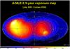 |
Fig. 1 AGILE-GRID 2.3 year all-sky exposure map in an Aitoff projection obtained with the FM event filter from all pointed-observations data (96 OBs). |
We describe the AGILE-GRID performances and the OB data archive in Sects. 2 and 3, the data analysis procedure in Sect. 4, and the variability analysis in Sect. 5. In Sect. 6 we present the results obtained, both the variability results and the catalogue of all detections in all OBs. We then discuss the results and report some final considerations in Sect. 7.
2. AGILE-GRID characteristics and calibration
The AGILE scientific payload consists of a silicon tracker imaging detector (Barbiellini et al. 2001, 2002; Prest et al. 2003), a CsI(Tl) mini-calorimeter detector (Labanti et al. 2006, 2009), and an anti-coincidence system (Perotti et al. 2006), which together form the Gamma-Ray Imaging Detector (GRID). It also features the X-ray coded mask silicon imaging detector SuperAGILE (Feroci et al. 2007). GRID is sensitive to photon energies in the 30 Mev−50 GeV energy band, with a wide FoV (2.5 sr in pointing mode) and accurate timing (2 μs), positional, and attitude information (15′ location accuracy for >10σ detection).
The GRID calibration has been updated since the launch (Pittori et al. 2009; Bulgarelli et al. 2010; Cattaneo et al. 2011, 2012; Chen et al. 2012). The GRID instrument energy-dependent point spread function (PSF), derived from in-flight calibrations, has a full-width at half-maximum (FWHM) of approximately 3.5° at 100 MeV and 0.7° at 1 Gev. The effective area is about 500 cm2 at 300 MeV, depending on the event filter. Both GRID PSF and effective area have a very good off-axis performance and are well calibrated up to 60°, showing very smooth variations with the angle relative to the instrument axis. The version of the response matrices used in this analysis (I0010) was developed through the analysis of in-flight data to introduce flux corrections to improve the spectral response, taking into account the energy dispersion. They were created by comparing the fluxes obtained with the AGILE likelihood analysis of the Vela pulsar in each energy bin, with those expected from the fluxes and spectra reported in the first Fermi catalogue (Chen et al. 2012, 2013).
The FM filter has a FoV of ~60° radius, which is different from the F4 filter used for the 1AGL, which was optimized only up to off-axis angles of ~40° radius.
The data analysis used the AGILE diffuse emission model (Giuliani et al. 2004) for diffuse γ-ray background as for the 1AGL, which substantially improves upon the previous one used by EGRET. It was obtained by using state-of-the-art maps of neutral hydrogen (Kalberla et al. 2005) and CO (Dame et al. 2001).
3. OB data archive
The AGILE baseline pointing plan during the pointing mode phase was defined before the beginning of each year’s announcement of opportunity cycle to reach the goals that maximize the scientific output of the mission. The AGILE Data Center (ADC), part of the ASI Science Data Center (ASDC) in Frascati, Italy1, is responsible for data reduction and scientific processing to create the official standard OB level-2 (LV2) data archive and distribute it to guest observers (GOs) or, when data become public, to the scientific community.
Raw data are routinely archived, transformed in FITS format (Trifoglio et al. 2008), and then processed using the official scientific data reduction and analysis software tasks (Bulgarelli et al. 2009; Chen et al. 2011b), which are integrated into an automatic quick-look (QL) pipeline system. The QL procedures perform data analysis on 1-, 2-, 3-, and 7-day time scales, including an automatic source detection and alert system (Bulgarelli et al. 2008). The final AGILE-GRID archive is created at the ADC after executing the OB standard analysis pipeline system. Both pipelines execute the event filter (based on a Kalman filter technique) for track identification, event direction, and energy reconstruction (Pittori & Tavani 2002; Giuliani et al. 2006)2. The official OB pointing mode archive was built after removing data corresponding to slews and occasional losses of fine-pointing attitude, and it includes LV2 products, the spacecraft (LOG) and event (EVT) files, and the level-3 (LV3) counts, exposure and diffuse model maps. The OB LV3 maps used in this analysis were created in the E > 100 MeV energy band, with a bin of 0.25° × 0.25°, selecting events within 60° of the mean OB pointing direction and excluding photons within 80° from the reconstructed satellite-Earth vector, to reduce γ-ray Earth-albedo contamination. This archive was created using the latest official version of the standard software and instrument response functions available at the time of the analysis3. The complete pointing mode OB archive4 is composed of 101 datasets with non-uniform exposures (from 1 to 45 days). We analysed the scientifically validated data archive that covers 2.3 years with 96 OBs (see Table 1), not including the first 5 OBs of the commissioning phase.
AGILE pointings in the period 9 July 2007 – 30 October 2009, corresponding to the 96 observation blocks (OB).
4. OB data analysis procedure
The procedure developed for the source analysis on the whole archive is based on point source detection at fixed preselected positions. The AGILE multi-source analysis task (ALIKE, Bulgarelli et al. 2009; Chen et al. 2011b), which we used to derive the best estimates of point source parameters, i.e. source significance, γ-ray flux, Galactic coordinates, and 95% confidence level (c.l.), is based on the maximum likelihood (ML) method. The ML method, used in previous γ-ray data analysis (Mattox et al. 1996) and for all recent AGILE and Fermi imaging results (see for instance Bulgarelli et al. 2012a,b; Nolan et al. 2012), compares measured counts in each pixel with the predicted counts derived from a γ-ray model composed of the Galactic diffuse model (see Sect. 2), an isotropic diffuse component, and point sources modelled according to the instrument PSF. To reduce systematic errors that arise because the data were taken far away from the source, only data within a circle of a given radius around each source were used. The significance of a source detection is given by the test statistic TS, defined as the likelihood ratio, that is expected to behave as χ in the null hypothesis for one single parameter that is to be optimized, i.e. the source flux. When m parameters must be optimized, the TS behaves as χ
 .
.
We divide the procedure in three main steps:
-
1)
the preliminary reanalysis of the 1AGL catalogue, mainly incomplex Galactic plane regions, based on LV3 deep maps fromthe merging of all data in the OB archive, more recent AGILEresults and including some high-latitude (|BII| > 10°) sources detected in QL automatic procedures on a weekly time scale. The creation of the updated source list for next step;
-
2)
the execution of a procedure based on the AGILE multi-source ML task on each OB LV3 map, first allowing source fluxes to vary while keeping source positions fixed, then allowing the source positions to vary;
-
3)
the revision of the source list, taking into account the new results at fixed positions, for example when a source
 is significantly changed (increased or decreased). The 95% c.l. contour obtained leaving the source position free was also checked to verify that contours of transient sources did not overlap the nearest source position.
where we used the defined above as detection significance parameter. The reanalysis of the 1AGL source positioning in step 1) is described in Sect. 4.1, followed by a description of step 2) in Sect. 4.2 and step 3) in Sect. 5.
4.1. Revision of the first AGILE-GRID catalogue based on the 2.3 yr dataset
The first AGILE catalogue (Pittori et al. 2009) was built using data collected during the first year of operations (July 2007 – June 2008), which includes half of cycle-1 of the AGILE GO program. The data analysis based on the conservative F4 filter, and the non-uniform sensitivity due to the inhomogeneous sky coverage during AGILE first year, limited the results in complex Galactic regions. We reanalyzed 1AGL sources in the Galactic plane regions, such as the Carina, LS I +61°303, Cygnus, Crux, and near the Galactic center, using the updated E > 100 MeV deep maps obtained from the merging of data up to October 2009 (Fig. 1) processed with the FM event filter. These maps were created using the event selections described in Sect. 3, using both 0.05° × 0.05° and 0.1° × 0.1° bins. We then built an updated reference list with improved source positions in these regions. We use the abbreviation “1AGLR” for the repositioned and new sources. First, we reanalyzed the low-significance (3 ≤ ≤ 4) detections from the 1AGL processing in the Carina (283° < LII < 292°), LS I +61°303 (130° < LII < 136°) and Scutum-Sagittarius (6° < LII < 36°) regions, as well as four high-latitude detections at  not included in the catalogue (three of which are included in the final source list: 1AGLR J0135+4759, 1AGLR J0222+4305, 1AGLR J0321+4137). We then reanalyzed sources from more recently refined AGILE results in the Galactic plane (Tavani et al. 2009b, 2009c; Sabatini et al. 2010; Giuliani et al. 2010; Bulgarelli et al. 2012a; Piano et al. 2012).
We performed an ML multi-source analysis on the updated deep maps for these sources, to obtain the average fluxes used in the subsequent individual OB analyses. Two examples of source repositioning are shown in Fig. 2: a simple case for the high-latitude source 1AGLR J1848+6709 and a complex case for the Carina region. For this last case new source positions obtained in the ML analysis where source positions were allowed to vary, the 95% c.l. contour radii for the sources for which they were closed and their  values are reported in Table 2. Two of these sources, 1AGLR J1022-5825 and 1AGLR J1107-6115, have been included in the list although they do not have a 95% c.l. contour from the ML analysis on deep maps. In these cases an additional value is shown, marked with an asterisk
  hereafter); the value was obtained by keeping source position fixed.
We included 1AGLR J1022-5825 because it is only slightly repositioned with respect to 1AGL J1022-5822, whose error radius did not include the new sources (1AGLR J1018-5852, 1AGLR J1022-5751 and AGL J1029-5836), however, and also because it is significant on a single OB (7800) map. It was possible to obtain a detection at  on this OB, with an acceptable 95% c.l. contour, when allowing the source position to vary. Moreover, by executing an ML analysis on deep maps, keeping its position and the parameters of all nearby sources fixed, we obtained
  . 1AGLR J1107-6115 was analogously included because of
  obtained with the deep maps at fixed position, and in some OBs with an ML analysis with the parameters of all nearby sources (and of the diffuse emission) fixed. AGL J1029-5836 and AGL J1045-5736 (a repositioning of 1AGL J1043-5749), which have a above 5, were instead not significant over the OB time scale, and so do not appear in the final table.
Revised γ-ray source list in the Carina region.
We also included seven sources detected in the QL processing on a weekly time scale with > 4 at medium-high galactic latitude (|BII | > 5°) to verify their significance on the non-uniform OB time scale. Only four of these were detected in our final processing and are included in the final source list described in Sect. 6 (they are 1AGLR J1625-2531, 1AGLR J1803-3941, 1AGLR J1833-2057, 1AGLR J2030-0617). The results from the QL processing on various time scales will be reported elsewhere.
We compared the results of each run with the input reference source list, revising it if needed. We took into account the 95% c.l. contours and the , to check in detail candidate sources at fluxes ~3.0 × 10⁻⁷ ph cm-2 s-1 in the Carina, LS I +61°303, Scutum and 1AGLR J1625-2531 regions. This review resulted in the final version of the list, which includes 90 candidate sources. This source list was used as input in the following step.
A better characterization of complex Galactic regions will be reported in a future catalogue, implementing a new automatic source blind search.
4.2. Analysis of individual OBs
The ALIKE task is an iterative procedure that evaluates all the ML parameters that are left free to vary for each source in the input source list. We decided to fix the positions of all sources to reduce the number of parameters evaluated by the ALIKE task during the ML analysis in each single OB. This reduces the task running-time and can improve the precision of the results (see Bulgarelli et al. 2012b). For the same reason, we also fixed the spectral indices to −2.1 for all sources except for the five well-known bright pulsars Geminga, Crab, Vela, 1AGL J1709-4428, and 1AGLR J2021+3653 (fixed to −1.66, −2.2, −1.69, −1.86 and −1.86, from 3EG; Hartman et al. 1999; Chen et al. 2012), for 1AGLR J0007+7307, 1AGLR J2031+4130 and 1AGL J1836+5923 (fixed to −1.85, −1.84 and −1.65, from 3EG and Bulgarelli et al. 2008, 2012a), for the high-mass X-ray binaries (HMXBs) LS I +61°303 and Cyg X-3 (fixed to −2.21 and −2.0 from 3EG and Bulgarelli et al. 2012a) and the supernova remnants (SNRs) W28, IC443 and W44 (fixed to −1.8, −2.01 and −1.93 from Giuliani et al. 2010, and 3EG respectively). These values are compatible with the 2FGL ones at the AGILE spectral resolution. In this analysis we used the ML task AG_multi2 included in the AGILE BUILD GRID_SCI_20 package and a circle of radius 10° for the ML analysis.
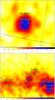 |
Fig. 2 Intensity maps of two 1AGL field refinements. In the first panel a simple case is shown, the high-latitude source 1AGL J1846+6714 repositioned to 1AGLR J1848+6709. The new smaller error circle is indicated in green inside the 1AGL circle, while the 2FGL J1849.4+6706 error ellipse is plotted in cyan. In the second panel a complex case is shown, the Carina region. New sources and new positions for 1AGL sources are indicated with a green circle, except for two sources for which no 95% c.l. contour has been obtained; their positions are indicated with crosses. The 1AGL error circles are indicated in black, the 2FGL error ellipses in cyan. |
To improve the reference list (in conjunction with the creation of a reprocessed OB archive with a new software version), in particular the multi-source detection in complex regions, all steps of the analysis were repeated five times. Finally, we selected the results obtained with the last processing with source positions kept fixed to the last version of the reference source list (see Sect. 5). Our goal was to refine multi-source detection in complex regions and add some high-latitude source, therefore we did not execute any automatic source detection process.
5. Detection selection and variability analysis
To investigate the variability within the OB dataset for established sources on deep maps and search for flaring episodes of sources with mean low significance, we analyzed the results from the last execution (the fifth) of the ML multi-source procedure on sources in the input reference list according to their significance and whether or not a 95% location contour could be found. We chose sources with either
-
1)
both a high-significance detection (
 ) from the deep map analysis and at least one OB detection with
  , or
, or -
2)
at least one detection with
 in a single OB. Moreover, we selected only sources with a 95% location contour from the deep map analysis (with a few exceptions, see Sect. 4.1).
Then we checked each single OB detection with  , inspecting the single OB intensity map and checking the size and shape of the source 95% c.l. contours from the ML at free position, if present, to verify whether it overlapped the nearest sources. We thus excluded eight sources from the final source list. All sources in the last version of the reference list that do not appear in the catalogue table were not significant in our analysis according to these criteria.
We used the method developed by McLaughlin et al. (1996) that was recently used in the analysis of 1AGL J2022+4032 data (Chen et al. 2011a) to study the OB-scale γ-ray flux variability of the selected sources and report the results in the next section. We computed three versions of the variability index. To calculate the traditional index V, we computed the weighted mean flux, its error, and the χ2 from the fluxes and errors in each OB. We evaluated the probability Q of having a value of  for a source assumed to have constant flux, and then defined the variability index V = −log Q. Sources with V < 0.5 were classified as non-variable, with 0.5 ≤ V < 1 as uncertain, and with V ≥ 1 as variable. A high V may indicate either strong flux variations or weak flux variations detected with small flux errors. Moreover, sources with a very small number of detections may also have low V (Nolan et al. 2003). We computed a second version of the variability index, Vsys3σ, by adding a 10% systematic component to each of the flux errors, where the 10% figure is based on Monte Carlo simulations, pre-flight beam tests and in-flight analysis of known sources. Finally, we computed a third version, Vsys2σ, of the V parameter as Vsys3σ, which also included the flux measures with
  , for which the ALIKE task produces a 95% c.l. flux upper limit (UL). In this case we set the flux errors to (FUL − Fi)/2. The two indices, Vsys3σ and Vsys2σ, which take systematic errors into account, will tend to be lower than V, which takes into account only the statistical error. These indices serve as the reference ones in our variability analysis, where Vsys2σ allows a larger detections sample for each source to provide some variability information for sources with few pointings. We excluded from the calculation of the indices the detections with a mean effective exposure lower than 9 × 106 cm2 s, corresponding to a small number of detections in OBs with a few days duration executed during the verification phase (July–November 2007).
 |
Fig. 3 Aitoff projection of the 54 distinct source positions detected on all pointed observations data (symbol colors indicate the variability parameter Vsys2σ of the 53 sources for which we define with blue the highest and with orange the lowest value. 1AGL J1238+0406 has a single detection and so is marked in black. Marker sizes are proportional to flux). |
We calculated a fourth variability index, Fsys, similar to that used in the Fermi catalogues (Abdo et al. 2009, 2010a), defined as a χ2 again including a 10% systematic error in the weights, to directly compare it with the Fermi 1FGL index. In our analysis each source has a different number of detections (Ndet) and so this parameter is expected to behave as the  distribution where the number of degrees of freedom (dof) is n = Ndet − 1. For this reason we considered the reduced Fsys (Reduc.Fsys = Fsys/Ndof), and compared it with the 1FGL variability index divided by 10 (i.e. the number of dof in 1FGL), and similarly with the 2FGL variability index divided by 23. We discuss in Sect. 7 a possible comparison with the 2FGL index as well, which is instead based on an ML ratio test statistic.
6. Results: the catalogue and source variability
Applying our selection criteria, we obtained a sample of 54 distinct sources (Fig. 3) with a total of 1209 OB detections. Eight 1AGL sources (2 high latitude and 6 on the galactic plane) were not detected in this processing either because of the low OB exposures and/or due to specific complex Galactic regions. We show information about the mean flux of these sources in Table 3, as obtained in the 1AGL.
We describe in the following the variability results (listed in Table 4) and the light curves of bright pulsars and of some prominent sources. We compared the light curves of sources with a known counterpart with those in the most recent Fermi catalogue (Nolan et al. 2012) for the time period common to both catalogues. The non-uniform exposures among the OBs together with the pointing strategy put strong constraints on the variability analysis.
1AGL sources not detected in this analysis.
The source and detections table5, Table 5, includes all the source flux measurements with ≥ 2 obtained for each of the 54 sources detected in this processing. In Table 5 we report the main parameters of the maximum detection for each source. These are the name, coordinates, the , the E > 100 MeV flux, the four variability indices described above and the number of detections, the confirmed counterparts and source class, if any, and other possible associations ordered according to the distance from the AGL source. We used the abbreviation 1AGLR for new sources and repositioned 1AGLs.
Below this row a list with all the flux measurements in each OB is shown with the observation parameters MJD start/stop, the OB number, the OB , the E > 100 MeV flux or the ULs for 2 ≤ ≤3, and the off-axis angle. The flux errors are statistical only, i.e. the results of our analysis. The association column is populated with sources from well-known catalogues that fall within error circles of radii given by the 95% statistical plus the 0.1° systematic, linearly added. In particular, sources from the 1AGL were the first included when present, then sources from the BZCAT (Massaro et al. 2008), from 3EG and 2FGL. Associations from known radio (Rinsland et al. 1975; Gregory et al. 1996), TeV (TEVCAT6), SNR (Green 2009), PSR (Manchester et al. 2003), and HMXB (Liu et al. 2006) catalogues were included for some sources without a previously confirmed counterpart (TeV emitting PWNs associated with bright pulsars are not shown).
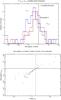 |
Fig. 4 Upper panel: histograms of the V (black unmarked line), Vsys2σ (red line with circles), and Vsys3σ (blue lines with triangles) parameters; lower panel: plot of Vsys2σ vs. the Reduc.Fsys. The vertical line in the upper plot is the threshold above which a source is variable (V ≥ 1) according to the V parameters. The horizontal line in the lower plot has the same meaning, while the vertical dashed line is the approximated extrapolation of a threshold for source variability for the Reduc.Fsys parameter, taking into account the correlation of both parameters. |
6.1. Variability results
The V index distributions are given in Fig. 4. They show that V values peak in the non-variable–uncertain ranges for all indices and that the V distribution is on average lower than the Vsys2σ (average values for V and Vsys2σ are 3.6 and 1.8), because of the obviously higher number of detections used for the Vsys2σ. The Vsys2σ and Reduc.Fsys gave similar results, as expected (Fig. 4), with a correlation factor 0.84. We then used this correlation to estimate a variability threshold for Reduc.Fsys extrapolated from the Vsys2σ threshold, considering the approximate intersection of the Vsys2σ = 1 line with the linear correlation plot. We estimated two possible linear correlation whose steepest and faintest slope included all points, obtaining a range of the Reduc.Fsys values at the intersection of 1.55−1.65, so we chose as threshold Reduc.Fsys ≈ 1.6. Details on the variability results obtained for different source classes are given in Table 4, for which we consider only sources with confirmed counterparts, except for 9 high-latitude sources associated with well known blazars also included among AGNs. The majority of variable sources are blazars according to all indices, the most variable one is 3C 454.3. The fraction of variable sources according to the Vsys2σ index is 20%, and a similar result, 22%, is obtained according to Vsys3σ.
However, the Fsys parameter and consequently V (which is based on the calculation of the χ2), depend on the ratio between mean flux and the standard deviation, so it is expected to be more likely to classify faint sources (flux <3.0 × 10⁻⁷ ph cm-2 s-1) or those near the Galactic plane as non-variable. Most of the unclassified sources are non-variable, but about half of the unclassified have an unconfirmed association with 2FGL pulsars.
Variability analysis results according to the V, Vsys3σ, and Vsys2σ indices, divided in to six main source classes.
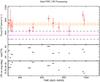 |
Fig. 5 Vela pulsar E > 100 MeV light curve in 10-8 ph cm-2 s-1 (upper panel), the |
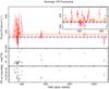 |
Fig. 6 Geminga pulsar E > 100 MeV light curve in 10-8 ph cm-2 s-1 (upper panel), the |
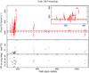 |
Fig. 7 Crab E > 100 MeV light curve (upper panel), the |
6.2. Light curves of bright pulsars
The light curves of the Vela and Geminga pulsars are shown in Figs. 5 and 6, and that of the Crab pulsar + nebula in Fig. 7. Vela and Geminga are the brightest among the non-variable sources. In all figures the mean off-axis angles and the in each OB are shown as well.
The weighted mean of the OB Vela fluxes is 86.8 ± 1.0 × 10⁻⁷ ph cm-2 s-1 while the value from the updated deep maps is 88.2 ± 0.9 × 10⁻⁷ ph cm-2 s-1, which is ~3.2σ higher than the mean value from the first AGILE catalogue, 78.0 ± 3.2 × 10⁻⁷ ph cm-2 s-1, according to the 1AGL error. We did not overplot the new mean value estimated from deep maps because the variability study is based on the mean of the OB fluxes. This new value, which should be considered as the new reference one, is higher than the previous value primarily because of the new instrument response functions, which compensate for the effect of energy dispersion, as well as the new filter calibrated up to a high off-axis angle. We obtained Vsys2σ = 0 and Fsys = 1.87, with 13 dof and expect a constant source to produce a value of Fsys ≤ 2.1 at 99% c.l.
A particular case is that of the Crab Nebula, which has recently been discovered to be a variable γ-ray source (see Tavani et al. 2011a,b; Abdo et al. 2011). In Fig. 6, first panel, we plot the Geminga light curve and its weighted mean OB flux value, 36.4 ± 0.9 × 10⁻⁷ ph cm-2 s-1, is shown. In Fig. 7 the Crab light curve shows the October 2007 flaring episode (MJD = 54 381.5, OB 4200), discussed in Tavani et al. (2011b), at a higher flux than for the 2010 flare. The Crab (Nebula + PSR) weighted mean OB flux value, 23.2 ± 0.9 × 10⁻⁷ ph cm-2 s-1, was calculated excluding seven OB during the 2007 flare (in the interval 54 368−54 396). We obtained Vsys2σ = 0.4 for Geminga and Vsys2σ = 3.4 for Crab. If we remove the 2007 flare peak from the Crab light curve we obtain Vsys2σ = 0.8, while if we remove all seven OB that cover the flare period that was excluded for the mean value estimate, we obtain Vsys2σ = 0.1, a non-variable value.
6.3. Long-term light curves of some prominent sources
We report here four long-term light curves, in the E > 100 MeV band, obtained for sources classified as variable, non-variable and a particular case of an uncertain one. We show in Figs. 8 and 9 the results for the two known blazars 3C 454.3 and PKS 1830-211. Light curves are shown including source detections with flux errors at 1σ, not including any systematic error.
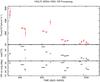 |
Fig. 8 3C 454.3 E > 100 MeV light curve in 10-8 ph cm-2 s-1 (upper panel), the |
Figure 8 shows the strong variability in the 3C 454.3 flux even at the OB time scale, and in particular the decreasing trend reported in Vercellone et al. (2010). This source has the strongest variability index Vsys2σ = 52.3. This confirms what was expected in Vercellone et al. (2004), a study of EGRET blazar activity and duty-cycle evaluation, which was based on a differently defined variability index.
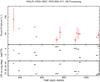 |
Fig. 9 1AGLR J1833-2057/PKS 1830-211 E > 100 MeV light curve in 10-8 ph cm-2 s-1 (upper panel), the |
1AGLR J1833-2057, associated to PKS 1830-211, is instead one of the fifteen new sources not included in 1AGL. Its light curve shows a detection in the period of the October 2009 flare (Striani et al. 2009), with a flux of (3.2 ± 0.8) × 10-7 ph cm-2 s-1, compatible with the one-week average flux (4.0 × 10⁻⁷ ph cm-2 s-1) reported in Donnarumma et al. (2011), based on data of the OB 8300 only, and shown to be three times weaker than the peak flare flux. This source is classified as non-variable according to all parameters, however, because of the flux averaging over the OB time scale. Other detections have been obtained, the most significant one in September 2008. This detection showed some source activity one year before the October 2009 flare, with a time scale between the two events similar to that between the 2009 and the following 2010 flare, which was also detected by Fermi (see discussion in Donnarumma et al. 2011).
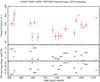 |
Fig. 10 1AGLR J2021+4030E > 100 MeV light curve in 10-8 ph cm-2 s-1 (upper panel), the |
In Fig. 10 we show the 1AGLR J2021+4030 light curve, a source that falls in the γ Cygni SNR region. The 1AGLR J2021+4030 variability on six-day time scale on pointing data (up to August 2009) was extensively discussed in Chen et al. (2011a), where values of 3.88 and 2.18 in E > 100 MeV were found for V and Vsys2σ, respectively, while low variability was detected at E > 400 MeV. The corresponding values in this paper are 5.9 and 2.70 and the light curve is compatible with that therein. 1AGLR J2021+4030 field is complex and there could be contribution to the variability from other γ-ray sources, that are possibly transient, in addition to LAT PSR J2021+4026 (see Chen et al. 2011a, for more details).
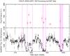 |
Fig. 11 1AGLR J2033+4057/Cyg X-3 E > 100 MeV light curve (upper panel) compared with the Swift/BAT 15 < E < 150 keV daily light curve. The plot shows six detections with |


Finally, we show in Fig. 11 the 1AGLR J2033+4057/ Cyg X-3 light curve together with the 15−150 keV daily light curve from Swift/BAT (Barthelmy et al. 2005). This plot is similar to those reported in Tavani et al. (2009c), Bulgarelli et al. (2012a), and Piano et al. (2012). Here we show the 1−2-day γ-ray flare times in the Pointing mode interval described there. Our detections correspond to the reported activity periods, and moreover a flux UL at = 2.7 (MJD = 54 591.5) is compatible with a short dip in the BAT hard X-ray light curve. We performed an additional ML analysis on a three-day time scale that found an additional low-significance ( ) short time scale γ-ray emission enhancement not included in Piano et al. (2012), which in fact reported the γ-ray activity on the 1−2-day time scale. Again our flux variations are averaged on longer time intervals, so that this source is only classified as uncertain in this analysis.
7. Discussion and conclusions
We reported the results of a variability analysis in the E > 100 MeV band of a catalogue of 54 sources obtained as an update of the 1AGL using the complete AGILE pointing mode OB archive. The new source list includes seven previously undetected sources with AGN counterparts and eight at low latitudes, while eight 1AGL sources were not detected in this analysis, two of which are at high latitude (1AGL J0657+4554 and 1AGL J1223+2851/WComae) and six are on the Galactic plane (1AGL J1044-5750, 1AGL J1412-6150, 1AGL J1746-3017, 1AGL J1815-1732, 1AGL J1901+0430, 1AGL J1923+1404).
We carried out the variability study by applying an ML analysis in each single OB without implementing any blind search for transient sources, among OBs with different exposure times.
This ML variability analysis, as discussed in Sect. 5, is known to be inadequate for the variability indices used (Nolan et al. 2003); however, the revised indices allowed us to distinguish variable from non-variable sources. All four variability indices defined in our analysis show that the majority of variable sources are blazars, consistent with the γ-ray source variability studies included in the first (1FGL) and second (2FGL) Fermi source catalogues.
A comparison with the 1FGL and 2FGL variability indices is shown in Fig. 12. The index from the 1FGL is a χ2 statistic calculated in the same manner as Fsys, while the 2FGL statistic is an ML ratio test statistic, defined in Nolan et al. (2012), which is distributed according to the  distribution in the null hypothesis of a constant source.
We associated our source list with those of 1FGL and 2FGL by a simple spatial cross-matching with radius 30′, yielding 46 and 49 sources in common, respectively. We used the Reduc.Fsys parameter because each source is detected in a different number of OBs (see Sect. 5).
For each source we defined a specific threshold for flux variability at 99% c.l. (as in Abdo et al. 2010a; Nolan et al. 2012) using the appropriate distribution for n dof. Thresholds range from 1.67 for a source with 31 detections to 6.2 for one with two detections, while the 1FGL and 2FGL thresholds are 2.32 and 1.81, respectively. Twelve sources out of 54 have fewer than five detections. Sources with a Reduc.Fsys higher than their own threshold (Reduc.Fsys >  ) are flagged as variable in the plot. We found that all of the AGILE variable sources, seven sources, are also variable in 1FGL except for two, the Crab and 1AGLR J2021+4030, while in 2FGL only 1AGLR J2021+4030 remains non-variable. The Crab case is clear: the AGILE pointing dataset included the very intense 2007 flare, with a peak flux three times the 1AGL mean flux, whose evolution is shown in various consecutive short-duration OBs (see Table 1), while fewer pointings are available from 2008 on. 1FGL included a flare affecting only the last of the 11 bins in the catalogue, while the 2FGL results show a much higher variability than for a lower mean flux with a smaller error. As discussed in Sect. 6.3, the variable emission from 1AGLR J2021+4030 might be generated by the contribution from other sources apart from the pulsar.
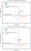 |
Fig. 12 Upper plot: Fermi 1FGL variability index divided by 10 vs. Reduc.Fsys for all detections associated with the 1FGL sources with a cross-matching with radius 30′, where colours correspond to source classes, blue for AGNs, black for HMXBs, red for PSRs, green for SNRs, light-blue for the unclassified ones, and orange for the three Special Cases Crab nebula + pulsar, 1AGLR J2021+4030 (γ Cygni region) and 1AGLR J1044-5944 (Eta Carinae). Markers correspond to AGILE variability type according to Reduc.Fsys, i.e. circles for non-variable and triangles for variable. The lower plot is obtained with association to the 2FGL catalogue with the same radius and shows the 2FGL index divided by 23. The black horizontal lines are the 1FGL and 2FGL variability thresholds, 2.32 and 1.81, while the dashed vertical lines correspond to the approximately extrapolated threshold (1.6) for the AGILE variability Reduc.Fsys parameter obtained from the correlation with the Vsys2σ parameter. |
Sources in the plots are divided into five main classes: AGN, PSRs, HMXBs, SNRs, and unclassified sources, while three particular cases are labelled separately (Crab PSR + nebula, 1AGLR J2021+4030 and 1AGLR J1044-5944). Only sources with confirmed (based on 1AGL and later AGILE results) counterparts were included in the specific classes, except for 9 high-latitude sources associated to well known blazar counterparts included as AGNs.
A good correlation with the 1FGL parameter is obtained for AGN whose diffuse γ-ray background is low, with a correlation factor of 0.98, which is expected for this class, taking into account their broad flux distribution and that at low fluxes (≤3.0 × 10⁻⁷ ph cm-2 s-1 for a typical AGN variability of 1−3 days) AGILE cannot detect variability. Lower correlation factors are obtained for PSRs and unclassified (0.01 and 0.05). The correlation factor considering all sources together is 0.98. The PSRs are all non-variable except for the two particular cases discussed above.
Lower values were also obtained for the correlation of Reduc.Fsys with the 2FGL index (0.88 for AGN, −0.28, 0.08 for PSRs and unclassified, while the value including all sources is 0.89), for AGN due also to 3C 273, whose variability index increased by a factor 4 from 1FGL to 2FGL (excluding it, the correlation factor for AGN is 0.97) and to 1AGLR J1625-2531 which became variable in 2FGL with an increase of a factor 10 in the variability index. We note the presence of an unclassified source within the AGN group in both plots. This is 1AGLR J2016+3644, a source within the Cygnus region that is non-variable according to Reduc.Fsys (and also Vsys2σ = 0.2), whose nearest Fermi sources are the unclassified 1FGL J2015.7+3708 (at 25′), 2FGL J2015.6+3709/MG2 J201534+3710 (at 27′), classified as a blazar of uncertain type, 2FGL J2018.0+3626 (unassociated, at 27′) and the SNR G74.9+1.2 (28′). All sources are slightly outside the 1AGLR J2016+3644 error circle, however. The comparison with the vertical dashed lines, the threshold at 1.6, shows that some sources marked with circles could be variable according to Vsys2σ, as confirmed by the exact numbers in Table 4. For instance, eight AGNs are variables according to Vsys2σ and ten blue points are rightward of the dashed line, while there are only five triangles.
The inhomogeneous exposure times among the OBs diminish the capability of studying the source variability in our data analysis; for this reason a similar analysis on the one-week time scale on the same pointing data archive would be useful to better classify the source variability, and will be reported in a future work.
More details on the ADC organization and tasks will be given in a future publication (Pittori et al., in prep.).
Software build version: BUILD GRID_STD_17 and BUILD GRID_SCI_19; calibration files version I0010.
Public OB archive is available at http://www.asdc.asi.it/mmia/index.php?mission=agilemmia
Available on-line at http://www.asdc.asi.it/agile1rcat
Acknowledgments
The AGILE Mission is funded by the Italian Space Agency (ASI) with scientific and programmatic participation by the Italian Institute of Astrophysics (INAF) and the Italian Institute of Nuclear Physics (INFN). Research partially supported through the ASI grants I/089/06/2, I/042/10/0 and I/028/12/0. The authors thank the anonymous referee for the useful suggestions.
References
- Abdo, A. A., Ackermann, M., Atwood, W. B., et al. 2008, Science, 322, 1218 [NASA ADS] [CrossRef] [PubMed] [Google Scholar]
- Abdo, A. A., Ackermann, M., Ajello, M., et al. 2009, ApJS, 183, 46 [NASA ADS] [CrossRef] [Google Scholar]
- Abdo, A. A., Ackermann, M., Ajello, M., et al. 2010a, ApJ, 715, 429 [NASA ADS] [CrossRef] [Google Scholar]
- Abdo, A. A., Ackermann, M., Ajello, M., et al. 2010b, Science, 329, 817 [NASA ADS] [CrossRef] [PubMed] [Google Scholar]
- Abdo, A. A., Ackermann, M., Ajello, M., et al. 2011, Science, 331, 739 [NASA ADS] [CrossRef] [PubMed] [Google Scholar]
- Atwood, W. B., Abdo, A. A., Ackermann, M., et al. 2009, ApJ, 697, 1071 [NASA ADS] [CrossRef] [Google Scholar]
- Barbiellini, G., Bordignon, G., Fedel, G., et al. 2001, AIP Conf. Proc. 587, 754 [Google Scholar]
- Barbiellini, G., Fedel, G., Liello, F., et al. 2002, NIM A, 490, 146 [Google Scholar]
- Barthelmy, S. D., Barbier, L. M., Cummings, J. R., et al. 2005, Space Sci. Rev., 120, 143 [NASA ADS] [CrossRef] [Google Scholar]
- Bulgarelli, A., Trifoglio, M., Gianotti, F., et al. 2008, Proc. Astronomical Data Analysis Software and Systems XVIII, Quebec, Canada, ADASS, ASP Conf. Ser. [Google Scholar]
- Bulgarelli, A., Chen, A., Giuliani, A., et al. 2009, GRID Scientific Analysis User Manual, AGILE-IFC-OP-009 [Google Scholar]
- Bulgarelli, A., Argan, A., Barbiellini, et al. 2010, NIM A, 614, 213 [NASA ADS] [CrossRef] [Google Scholar]
- Bulgarelli, A., Tavani, M., Chen, A., et al. 2012a, A&A, 538, A63 [NASA ADS] [CrossRef] [EDP Sciences] [Google Scholar]
- Bulgarelli, A., Chen, A., Tavani, M., et al. 2012b, A&A, 540, A79 [NASA ADS] [CrossRef] [EDP Sciences] [Google Scholar]
- Cattaneo, P. W., Argan, A., Boffelli, F., et al. 2011, NIM A, 630, 251 [NASA ADS] [CrossRef] [Google Scholar]
- Cattaneo, P. W., Rappoldi, A., Argan, A., et al. 2012, SPIE, 8443E, 4D [Google Scholar]
- Chen, A., Piano, G., Tavani, M., et al. 2011a, A&A, 525, A33 [NASA ADS] [CrossRef] [EDP Sciences] [Google Scholar]
- Chen, A., Bulgarelli, A., Contessi, T., et al. 2011b, GRID Scientific Analysis User Manual, AGILE-IFC-OP-009_Build-21 (http://agile.asdc.asi.it/publicsoftware.html) [Google Scholar]
- Chen, A., Argan, A., Bulgarelli, A., et al. 2012, SPIE, 8443E, 4E [Google Scholar]
- Chen, A., Argan, A., Bulgarelli, A., et al. 2013, A&A, submitted [Google Scholar]
- Dame, T. M., Hartmann, D., & Thaddeus, P. 2001, ApJ, 547, 792 [NASA ADS] [CrossRef] [Google Scholar]
- Donnarumma, I., De Rosa, A., Vittorini, V., et al. 2011, ApJ, 736, L30 [NASA ADS] [CrossRef] [Google Scholar]
- Feroci, M., Costa, E., Soffitta, P., et al. 2007, NIM A, 581, 728 [NASA ADS] [CrossRef] [Google Scholar]
- Gianotti, F., & Trifoglio, M. 2001, in Astronomical Data Analysis Software and Systems X, eds. F. R. Harnden, Jr., F. A., Primini, & H. E., Payne, ASP Conf. Ser., 238, 245 [Google Scholar]
- Giuliani, A., Chen, S., Mereghetti, et al. 2004, Mem. SAIt Suppl., 5, 135 [Google Scholar]
- Giuliani, A., Cocco, V., Mereghetti, S., Pittori, C., & Tavani, M. 2006, NIM A, 568, 692 [NASA ADS] [CrossRef] [Google Scholar]
- Giuliani, A., Tavani, M., Bulgarelli, A., et al. 2010, A&A, 516, L11 [Google Scholar]
- Green, D. A. 2009, BASI, 37, 45 [NASA ADS] [Google Scholar]
- Gregory, P. C., Scott, W. K., Douglas, K., & Condon, J. J. 1996, ApJS, 103, 427 [NASA ADS] [CrossRef] [Google Scholar]
- Hartman, R. C., Bertsch, D. L., Bloom, S. D., Chen, A. W., et al. 1999, ApJS, 123, 79H [NASA ADS] [CrossRef] [Google Scholar]
- Kalberla, P. M. W., Burton, W. B., Hartmann, D., et al. 2005, A&A, 440, 775 [NASA ADS] [CrossRef] [EDP Sciences] [Google Scholar]
- Labanti, C., Marisaldi, M., Fuschino, F., et al. 2006, SPIE, 6266, 62663Q [Google Scholar]
- Labanti, C., Marisaldi, M., Fuschino, F., et al. 2009, NIM A, 598, 470 [NASA ADS] [CrossRef] [Google Scholar]
- Liu, Q. Z., van Paradijs, J., & van den Heuvel, E. P. J. 2006, A&A, 455, 1165 [NASA ADS] [CrossRef] [EDP Sciences] [Google Scholar]
- Manchester, R. N., Hobbs, A. T., & Hobbs, M. 2005, AJ, 129, 1993 [NASA ADS] [CrossRef] [Google Scholar]
- Massaro, E., Giommi, P., Leto, L., et al. 2009, A&A, 495, 691 [NASA ADS] [CrossRef] [EDP Sciences] [Google Scholar]
- Mattox, J. R., Bertsch, D. L., Chiang, J., et al. 1996, ApJ, 461, 396 [NASA ADS] [CrossRef] [Google Scholar]
- McLaughlin, M. A., Mattox, J. R., Cordes, J. M., & Thompson, D. J. 1996, ApJ, 473, 763 [NASA ADS] [CrossRef] [Google Scholar]
- Michelson, P. F. 2008, APS Meeting Abstracts, TSSP, L2002 [Google Scholar]
- Morselli, A., Argan, A., Barbiellini, G., et al. 2013, NUPH B, in press [Google Scholar]
- Nolan, P. L., Tompkins, W. F., Grenier, I. A., et al. 2003, ApJ, 597, 615 [NASA ADS] [CrossRef] [Google Scholar]
- Nolan, P. L., Abdo, A. A., Ackermann, M., et al. 2012, ApJS, 199, 31 [NASA ADS] [CrossRef] [Google Scholar]
- Rinsland, C., Dixon, R., & Kraus, J. 1975, AJ, 80, 759 [NASA ADS] [CrossRef] [Google Scholar]
- Paredes, J. M., Mart, J., & Torres, D. F. 2005, Ap&SS, 297, 223 [NASA ADS] [CrossRef] [Google Scholar]
- Perotti, F., Fiorini, M., Incorvaia, S., Mattaini, E., & Sant’Ambrogio, E. 2006, NIM A, 556, 228 [NASA ADS] [CrossRef] [Google Scholar]
- Piano, G., Tavani, M., Vittorini, V., et al. 2012, A&A, 545, A110 [NASA ADS] [CrossRef] [EDP Sciences] [Google Scholar]
- Pittori, C., & Tavani, M. 2002, NIM A, 488, 295 [NASA ADS] [CrossRef] [Google Scholar]
- Pittori, C., Verrecchia, F., Chen, A. W., et al. 2009, A&A, 506, 1563 [NASA ADS] [CrossRef] [EDP Sciences] [Google Scholar]
- Prest, M., Barbiellini, G., Bordignon, G., et al. 2003, NIM A, 501, 280 [NASA ADS] [CrossRef] [Google Scholar]
- Romero, G. E., Benaglia, P., Torres, D. F., et al. 1999, A&A, 348, 868 [NASA ADS] [Google Scholar]
- Sabatini, S., Tavani, M., Striani, E., et al. 2010, ApJ, 712, 10 [Google Scholar]
- Striani, E., Verrecchia, F., Pittori, C., et al. 2009, ATel, 2242, 1 [NASA ADS] [Google Scholar]
- Tavani, M. 2011, A&AS, 217, 43406 [Google Scholar]
- Tavani, M., Barbiellini, G., Argan, A., et al. 2008, for the AGILE Collaboration, NIM A, 588, 52 [NASA ADS] [CrossRef] [Google Scholar]
- Tavani, M., Barbiellini, G., Argan, A., et al. 2009a, for the AGILE Collaboration, A&A, 502, 995 [NASA ADS] [CrossRef] [EDP Sciences] [Google Scholar]
- Tavani, M., Sabatini, S., Pian, E., et al. 2009b, ApJ, 698, L142 [Google Scholar]
- Tavani, M., Bulgarelli, A., Piano, G., et al. 2009c, Nature, 462, 620 [NASA ADS] [CrossRef] [PubMed] [Google Scholar]
- Tavani, M., Giuliani, A., Chen, A. W., et al. 2010, ApJ, 710, L151 [NASA ADS] [CrossRef] [Google Scholar]
- Tavani, M., Bulgarelli, A., Vittorini, V., et al. 2011, Science, 331, 736 [NASA ADS] [CrossRef] [PubMed] [Google Scholar]
- Thompson, D. J. 2008, RPPh, 71k, 6901 [Google Scholar]
- Thompson, D. J., Bertsch, D. L., Fichtel, C. E., et al. 1993, ApJS, 86, 629 [NASA ADS] [CrossRef] [Google Scholar]
- Torres, D. F., Romero, G. E., Combi, J. A., et al. 2001, A&A, 370, 468 [NASA ADS] [CrossRef] [EDP Sciences] [Google Scholar]
- Trifoglio, M., Bulgarelli, A., Gianotti, F., et al. 2008, Proc. SPIE, 7011, 70113E [CrossRef] [Google Scholar]
- Vercellone, S., Soldi, S., Chen, A. W., & Tavani, M. 2004, MNRAS, 353, 890 [NASA ADS] [CrossRef] [Google Scholar]
- Vercellone, S., D’Ammando, F., Vittorini, V., et al. 2008, ApJ, 676, L13 [NASA ADS] [CrossRef] [Google Scholar]
- Vercellone, S., D’Ammando, F., Vittorini, V., et al. 2010, ApJ, 712, 405 [NASA ADS] [CrossRef] [Google Scholar]
- Verrecchia, F., Pittori, C., Bulgarelli, A., et al. 2011, Fermi Symp. Proc., eConf C110509 [arXiv:1111.0025] [Google Scholar]
- Vittorini, V., Tavani, M., Pucella, G., et al. 2010, ApJ, 732, L22 [Google Scholar]
All Tables
AGILE pointings in the period 9 July 2007 – 30 October 2009, corresponding to the 96 observation blocks (OB).
Variability analysis results according to the V, Vsys3σ, and Vsys2σ indices, divided in to six main source classes.
All Figures
|
Fig. 1 AGILE-GRID 2.3 year all-sky exposure map in an Aitoff projection obtained with the FM event filter from all pointed-observations data (96 OBs). |
| In the text | |
|
Fig. 2 Intensity maps of two 1AGL field refinements. In the first panel a simple case is shown, the high-latitude source 1AGL J1846+6714 repositioned to 1AGLR J1848+6709. The new smaller error circle is indicated in green inside the 1AGL circle, while the 2FGL J1849.4+6706 error ellipse is plotted in cyan. In the second panel a complex case is shown, the Carina region. New sources and new positions for 1AGL sources are indicated with a green circle, except for two sources for which no 95% c.l. contour has been obtained; their positions are indicated with crosses. The 1AGL error circles are indicated in black, the 2FGL error ellipses in cyan. |
| In the text | |
|
Fig. 3 Aitoff projection of the 54 distinct source positions detected on all pointed observations data (symbol colors indicate the variability parameter Vsys2σ of the 53 sources for which we define with blue the highest and with orange the lowest value. 1AGL J1238+0406 has a single detection and so is marked in black. Marker sizes are proportional to flux). |
| In the text | |
|
Fig. 4 Upper panel: histograms of the V (black unmarked line), Vsys2σ (red line with circles), and Vsys3σ (blue lines with triangles) parameters; lower panel: plot of Vsys2σ vs. the Reduc.Fsys. The vertical line in the upper plot is the threshold above which a source is variable (V ≥ 1) according to the V parameters. The horizontal line in the lower plot has the same meaning, while the vertical dashed line is the approximated extrapolation of a threshold for source variability for the Reduc.Fsys parameter, taking into account the correlation of both parameters. |
| In the text | |
|
Fig. 5 Vela pulsar E > 100 MeV light curve in 10-8 ph cm-2 s-1 (upper panel), the |
| In the text | |
|
Fig. 6 Geminga pulsar E > 100 MeV light curve in 10-8 ph cm-2 s-1 (upper panel), the |
| In the text | |
|
Fig. 7 Crab E > 100 MeV light curve (upper panel), the |
| In the text | |
|
Fig. 8 3C 454.3 E > 100 MeV light curve in 10-8 ph cm-2 s-1 (upper panel), the |
| In the text | |
|
Fig. 9 1AGLR J1833-2057/PKS 1830-211 E > 100 MeV light curve in 10-8 ph cm-2 s-1 (upper panel), the |
| In the text | |
|
Fig. 10 1AGLR J2021+4030E > 100 MeV light curve in 10-8 ph cm-2 s-1 (upper panel), the |
| In the text | |
|
Fig. 11 1AGLR J2033+4057/Cyg X-3 E > 100 MeV light curve (upper panel) compared with the Swift/BAT 15 < E < 150 keV daily light curve. The plot shows six detections with |
| In the text | |
|
Fig. 12 Upper plot: Fermi 1FGL variability index divided by 10 vs. Reduc.Fsys for all detections associated with the 1FGL sources with a cross-matching with radius 30′, where colours correspond to source classes, blue for AGNs, black for HMXBs, red for PSRs, green for SNRs, light-blue for the unclassified ones, and orange for the three Special Cases Crab nebula + pulsar, 1AGLR J2021+4030 (γ Cygni region) and 1AGLR J1044-5944 (Eta Carinae). Markers correspond to AGILE variability type according to Reduc.Fsys, i.e. circles for non-variable and triangles for variable. The lower plot is obtained with association to the 2FGL catalogue with the same radius and shows the 2FGL index divided by 23. The black horizontal lines are the 1FGL and 2FGL variability thresholds, 2.32 and 1.81, while the dashed vertical lines correspond to the approximately extrapolated threshold (1.6) for the AGILE variability Reduc.Fsys parameter obtained from the correlation with the Vsys2σ parameter. |
| In the text | |
Current usage metrics show cumulative count of Article Views (full-text article views including HTML views, PDF and ePub downloads, according to the available data) and Abstracts Views on Vision4Press platform.
Data correspond to usage on the plateform after 2015. The current usage metrics is available 48-96 hours after online publication and is updated daily on week days.
Initial download of the metrics may take a while.