| Issue |
A&A
Volume 557, September 2013
|
|
|---|---|---|
| Article Number | A55 | |
| Number of page(s) | 19 | |
| Section | Astronomical instrumentation | |
| DOI | https://doi.org/10.1051/0004-6361/201321668 | |
| Published online | 29 August 2013 | |
Photometry of supernovae in an image series: methods and application to the SuperNova Legacy Survey (SNLS)⋆
1
Laboratoire de Physique Nucléaire et des Hautes Energies, UPMC Univ. Paris
6, UPD Univ. Paris 7, CNRS IN2P3, 4
place Jussieu, 75005
Paris, France
e-mail: This email address is being protected from spambots. You need JavaScript enabled to view it.
2
Department of Physics and Astronomy, University of
Victoria, Elliott Building 101,
3800 Finnerty Road (Ring Road), Victoria, BC, Canada
3
Integral Data Center for Astrophysics, Department of Astronomy,
University of Geneva ch. d’Écogia 16, 1290
Versoix,
Switzerland
Received:
8
April
2013
Accepted:
12
June
2013
Abstract
Aims. We present a technique to measure lightcurves of time-variable point sources on a spatially structured background from imaging data. The technique was developed to measure lightcurves of SNLS supernovae in order to infer their distances. This photometry technique performs simultaneous point spread function (PSF) photometry at the same sky position on an image series.
Methods. We describe two implementations of the method: one that resamples images before measuring fluxes, and one which does not. In both instances, we sketch the key algorithms involved and present the validation using semi-artificial sources introduced in real images in order to assess the accuracy of the supernova flux measurements relative to that of surrounding stars. We describe the methods required to anchor these PSF fluxes to calibrated aperture catalogs, in order to derive SN magnitudes.
Results. We find a marginally significant bias of 2 mmag of the after-resampling method, and no bias at the mmag accuracy for the non-resampling method. Given surrounding star magnitudes, we determine the systematic uncertainty of SN magnitudes to be less than 1.5 mmag, which represents about one third of the current photometric calibration uncertainty affecting SN measurements. The SN photometry delivers several by-products: bright star PSF flux measurements which have a repeatability of about 0.6%, as for aperture measurements; we measure relative astrometric positions with a noise floor of 2.4 mas for a single-image bright star measurement; we show that in all bands of the MegaCam instrument, stars exhibit a profile linearly broadening with flux by about 0.5% over the whole brightness range.
Key words: techniques: image processing / supernovae: general / astrometry / techniques: photometric
Based on observations obtained with MegaPrime/MegaCam, a joint project of CFHT and CEA/DAPNIA, at the Canada-France-Hawaii Telescope (CFHT) which is operated by the National Research Council (NRC) of Canada, the Institut National des Sciences de l’Univers of the Centre National de la Recherche Scientifique (CNRS) of France, and the University of Hawaii.
© ESO, 2013
1. Introduction
Measuring lightcurves of variable stars is nowadays mostly carried out by performing photometry in an image series. This usually does not reduce to just gathering measurements obtained independently on each image, because one can take advantage of at least two specific features: most of the stars in the image series are not variable, and the relative positions of astronomical sources are constant in the image series, with a subset possibly affected by significant proper motions.
Most of the proposed implementations of lightcurve measurements are able to detect flux variations, below the fluctuations due to atmospheric extinction or instrumental response variation, that typically affects a single-image or single-epoch measurement. Relying on the assumption that stars are on average non-variable allows one to correct for these noise sources on an image per image basis. Measurements aimed at detecting micro-lensing, planet transits, or more generally measuring small luminosity variations, are commonly characterized by the smallest relative flux variation they can detect for their brightest stars. Ground-based instruments can reach the milli-magnitude level (e.g. Montalto et al. 2007), while space-based instruments approach 10-5 (e.g. Jenkins et al. 2010).
Our variable-source photometry pipeline aims at measuring lightcurves of supernovae (SNe), in order to infer luminosity distances from those, in the context of ground-based observations. This requires to derive some apparent luminosity indicator from the data that is both accurate (i.e. precisely calibrated) and limited only by shot noise (because distant supernovae are faint). Supernova observations could in principle be directly calibrated to standard stars. This route is however inefficient because a sizable fraction of observing nights is non-photometric, i.e. the temporal or spatial variability of atmospheric extinction is too large to allow one to reliably assume that science and calibration targets were observed under sufficiently similar conditions. Hence, most ground-based supernova surveys calibrate their supernovae via a two-step process: measuring the ratio of SN flux to some surrounding stars (step 1), and measuring the fluxes of these surrounding stars with respect to some standards, usually in a subset of images (step 2). As these standards are usually secondary standards, commonly the Landolt catalog (Landolt 1992) or the Smith catalog, (Smith et al. 2002), the “relay stars” in SN fields are called tertiary stars. This two-step process allows one to rescue non-photometric observations of the SN, again under the assumption that tertiary stars are on average non-variable. Note, however, that variable stars can be detected and ignored. The key performances of an SN lightcurve pipeline is no longer the smallest detectable luminosity variation, but rather the statistical efficiency1 of the supernova measurements and the fidelity (on average) of the ratio of supernova flux to that of neighbouring stars. These two qualities are usually called precision and accuracy respectively.
In this paper, we will concentrate on the first measurement step, i.e. measuring the ratio of SN fluxes to that of tertiary stars, in the framework of the SuperNova Legacy Survey (SNLS, described in Sect. 2). We will discuss as well the comparison of obtained instrumental magnitudes to calibrated magnitudes obtained at step 2, which turns out to be more subtle than one might naively think. We will not discuss here the derivation of magnitudes of tertiary stars on a photometric system accurately related to physical fluxes, but rather point interested readers to Betoule et al. (2013, and references therein) for the data set discussed in this paper, and to Ivezić et al. (2007), Tucker et al. (2006, and references therein) for a parallel work on the SDSS SN survey, with some updates in Betoule et al. (2013).
Regarding the SN-to-tertiary stars measurement, our approach consists in fitting a time-variable point source on top of a time-independent galaxy image to the image series. We propose two incarnations of the procedure, one which requires resampling the images prior to the fit, and a second one which does not. The former was used for past SNLS publications (Astier et al. 2006; Guy et al. 2010), and the latter is very similar to the “Scene modeling” described in Holtzman et al. (2008) that was developed for the SDSS SN survey.
SN cosmology now requires accurate SN fluxes: with the current sample of ~500 well-measured SNe distances, photometric calibration uncertainties, typically better than 0.01 mag, contribute as much as random errors (shot noise and SN variability) to the cosmological parameters uncertainties (Conley et al. 2011; Sullivan et al. 2011). Since biases of SN flux measurements relative to field stars contribute to the overall cosmology uncertainty budget in the same way as photometric calibration uncertainties, SN photometry is now to be challenged at the few mmag level. In this work, we report on tests and effects at this level of accuracy, or better. Random errors affecting SN measurements are much larger, but average out.
The plan of this paper goes as follows: we first briefly describe the SNLS (Sect. 2) and then sketch (Sect. 3) the pre-reduction steps applied to images prior to SN photometry. We compare our approach with others that have been used in Sect. 4. We then describe our two implementations of the SN photometry, the “resampled simultaneous photometry” (RSP thereafter, Sect. 5) and the “direct simultaneous photometry” (DSP thereafter, Sect. 6). For the latter we detail the calculation of the simultaneous astrometric solution and the influence of atmospheric refraction. We then enter into the tests of both methods using simulations that heavily rely on real images (Sect. 7). How we relate instrumental magnitudes of tertiaries to calibrated magnitudes of the same stars is described in Sect. 8. We assess the quality of SN photometry in Sect. 9. We discuss the variation of PSF size with star brightness in Sect. 10. We briefly sketch the salient technical points of the implementation in Sect. 11, and conclude in Sect. 12.
2. The SNLS
We deliver here the minimum information about the survey required for what follows, see Astier et al. (2006) for more details. The SNLS was a two-prong survey: the photometry was acquired within the deep survey of the Canada-France Hawaii Telescope Legacy Survey (CFHTLS2), conducted on the CFHT from 2003 to 2008, using the then new 1 deg2 imager MegaCam. SNLS also conducted a spectroscopic survey relying mostly on VLT, Gemini and Keck that we will not discuss further. MegaCam (Boulade et al. 2003) gathers 36 back-illuminated thinned CCDs (E2V CCD42-90) of 2048 × 4612 pixel2 with a plate scale of 0.185′′/pixel. This plate scale delivers images which sample typical PSFs with more than 4 pixels full width at half maximum (FWHM), falling to ~2.5 for the best image quality. These CCDs are arranged in 4 rows of 9 chips, each covering 6.3 × 14.2 arcmin2. The deep CFHTLS survey consisted in monitoring 4 to 5 times per lunation in the griz bands, 4 pointings spread in right ascension, as long as they remained visible. Each visit typically consisted in 5 to 8 consecutive images with exposure times of a few hundred seconds, and ditherings of at most 250 pixels in right ascension and 1000 pixels in declination. Most of the observing nights also have calibration exposures of Landolt fields, in ugriz bands. The four science fields, (see Table 1 in Astier et al. 2006) were selected for their low Galactic extinction, and hence have a low stellar density. MegaCam observations are grouped in “runs”, lasting 14−18 nights in a row, centered on new moon. The camera is removed from the telescope during bright time. MegaCam observations are acquired by the observatory staff according to observers’ requests. Depending on band and field, the CFHTLS deep survey has delivered 500 to 800 individual exposures that are used to measure lightcurves of supernovae.
All images gathered with MegaCam have very similar orientations (relative rotations are on the order of 0.2° rms, but much less within a run), and the x and y coordinates of the CCDs are fairly well aligned with right ascension and declination. At the beginning of the survey, the image quality was typically 20% worse in the corners of the focal plane than in the center. This improved to ~10% after the flip of the L3 lens of the image corrector in Dec. 2004. In July 2007, the i filter was accidentally broken, and a replacement filter was procured within 3 months, slightly different from the original, which we call i2 in what follows. No SN event has data in both filters.
3. Pre-reduction and PSF modeling
MegaCam images are processed at CFHT before release using the Elixir pipeline (Magnier & Cuillandre 2004). This set of tools assembles flat-field frames from twilight images from a whole MegaCam run and applies those consistently to all exposures. It also extracts fringe patterns from all science images in i and z bands and subtracts those. Images are delivered with an astrometry to ~1′′.
Some processing of the images is required before they can enter the SN photometry pipeline. We typically need:
-
some estimates of data quality, e.g. image quality (IQ), objectscounts, a preliminary estimate of the photometric zero point inorder to assess the atmospheric extinction;
-
a map of pixel weights initialized from inverse sky variance and flat-field frames. This map also identifies the pixels to be ignored for measurements, typically from CCD defects, saturation, cosmic rays and satellite trails;
-
a world coordinate system (WCS) for each image, obtained from matching the image catalog to that of a deep image stack itself anchored to the USNO catalog to set scale and orientation. We only rely on relative positions from these WCSs in order to match catalogs from different images of the same field;
-
a PSF model for each image allowing for spatial variations.
The reductions described in this paragraph are carried out independently for each CCD (2048 × 4612 pixels, 6.2 × 14.2 arcmin).
Some images were acquired at CFHT for the survey, but are not part of the CFHTLS data sample because of their poor quality. We anyway collect those poor quality images and apply two quality cuts: we reject images with IQ > 3.5 (defined in Eq. (2) below, and the median IQ is around 2), or with an atmospheric extinction above ~2 mag from the average. In both instances, these images do not convey a significant amount of information for SN lightcurves.
3.1. Image catalog and sky background
We use SExtractor (Bertin & Arnouts 1996) to
build a first image catalog, and obtain a “segmentation map” (i.e. a map of pixels
attributed to detected objects). We enlarge the footprint of objects by 5 pixels, and then
compute a sky background map using only unmasked pixels, using an algorithm similar to the
SExtractor one. We then subtract this smooth background component, and compute the
Gaussian-weighted first and second moments of all detections. The second moments of the
Gaussian weighting function are iteratively adjusted to the ones of each object, i.e. the
matrix of weighted second moments should satisfy: ![Mathematical equation: \begin{eqnarray} \label{eq:gaussian-moments}&&{\bf M}_{\rm g} = 2 \frac{\sum_{\rm pixels} ({\boldsymbol x_i}-{\boldsymbol x_{\rm c}}) ({\boldsymbol x_i}-{\boldsymbol x_{\rm c}})^{\rm T} {\bf W}_{\rm g}({\boldsymbol x_i}) I_i}{\sum_{\rm pixels} {\bf W}_{\rm g}({\boldsymbol x_i}) I_i} \\ &&{\bf W}_{\rm g}({\boldsymbol x_i}) \equiv \exp \left[ -\frac{1}{2} ({\boldsymbol x_i}-{\boldsymbol x_{\rm c}})^{\rm T}{\bf M}_{\rm g}^{-1}({\boldsymbol x_i}-{\boldsymbol x_{\rm c}}) \right ] \nonumber \end{eqnarray}](/articles/aa/full_html/2013/09/aa21668-13/aa21668-13-eq18.png) (1)where
xi are pixel coordinates,
xc the Gaussian weighted centroid obtained
similarly, and Ii is the (sky subtracted)
image value at pixel i. This iterative adjustment of second moments
mostly fails on extremely sharp detections typically due to image defects or cosmic rays.
The algorithm often diverges on blended objects, which then do not get second moments
measurements. Equation (1) is the normal
equation for second moments of a least squares fit of a 2D-Gaussian to the image,
assuming a stationary noise (i.e. position-independent). Ignoring the
contribution of the object to pixel variance makes the relative weights of pixels
independent of the star flux, and hence ensures that the inadequacy of the Gaussian PSF to
describe the actual star shapes does not cause a flux-dependent shift of these Gaussian
second moments. We have checked on simulated images with a non-Gaussian PSF that this size
estimator is independent of brightness at the 10-4 level.
(1)where
xi are pixel coordinates,
xc the Gaussian weighted centroid obtained
similarly, and Ii is the (sky subtracted)
image value at pixel i. This iterative adjustment of second moments
mostly fails on extremely sharp detections typically due to image defects or cosmic rays.
The algorithm often diverges on blended objects, which then do not get second moments
measurements. Equation (1) is the normal
equation for second moments of a least squares fit of a 2D-Gaussian to the image,
assuming a stationary noise (i.e. position-independent). Ignoring the
contribution of the object to pixel variance makes the relative weights of pixels
independent of the star flux, and hence ensures that the inadequacy of the Gaussian PSF to
describe the actual star shapes does not cause a flux-dependent shift of these Gaussian
second moments. We have checked on simulated images with a non-Gaussian PSF that this size
estimator is independent of brightness at the 10-4 level.
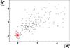 |
Fig. 1 Gaussian-weighted second moments from a single typical image, with the found star clump and the star selection (red points within the ellipse). |
The Gaussian-weighted second moments of stars tend to cluster in the
 plane. The shape of the star clump (due to
the variation of PSF across the CCD) is modeled as a 2-D Gaussian distribution and stars
are selected within a 5-σ ellipse, as shown in Fig. 1. We compute the average second moment matrix of found stars
plane. The shape of the star clump (due to
the variation of PSF across the CCD) is modeled as a 2-D Gaussian distribution and stars
are selected within a 5-σ ellipse, as shown in Fig. 1. We compute the average second moment matrix of found stars
 and define the image quality as:
 ![Mathematical equation: \begin{equation} \sigma_{\rm IQ}\equiv \sqrt[4]{\det ({\bf \bar{M}})} \label{eq:iq-definition} \end{equation}](/articles/aa/full_html/2013/09/aa21668-13/aa21668-13-eq26.png) (2)σIQ hence refers
to a Gaussian rms rather than FWHM, and is expressed in pixel units. A 0.8′′ FWHM seeing,
typical for the CFHTLS observations, translates to
σIQ ~ 2 with our definition. We define a set of circular
apertures in units of σIQ, and measure the fluxes of all
detections in these apertures, keeping track of bad or saturated pixels, and pixels
attributed to other detections. These aperture catalogs constitute the basic bricks of the
tertiary catalogs which are presented in Betoule et al.
(2013). Images in which the star cluster cannot be found are ignored for further
processing. These failures are usually due to massive extinction or severe guiding errors.
The WCSs are computed from the Gaussian-weighted positions.
(2)σIQ hence refers
to a Gaussian rms rather than FWHM, and is expressed in pixel units. A 0.8′′ FWHM seeing,
typical for the CFHTLS observations, translates to
σIQ ~ 2 with our definition. We define a set of circular
apertures in units of σIQ, and measure the fluxes of all
detections in these apertures, keeping track of bad or saturated pixels, and pixels
attributed to other detections. These aperture catalogs constitute the basic bricks of the
tertiary catalogs which are presented in Betoule et al.
(2013). Images in which the star cluster cannot be found are ignored for further
processing. These failures are usually due to massive extinction or severe guiding errors.
The WCSs are computed from the Gaussian-weighted positions.
3.2. PSF modeling
The star catalog from each image is used as input for modeling the PSF. We roughly follow
the strategy of DAOPHOT (Stetson 1987): modeling an
analytic point spread function (PSF) and complement it with pixelized correction at the
same sampling as the images. The analytic part offers the advantage that it accurately
describes the dependence of the PSF with respect to the object position within the central
pixel, and the non-analytic part accommodates departures from the analytic shape, such as
asymetries and guiding errors. For the analytic part, we chose an elliptical Moffat PSF
(Moffat 1969):
![Mathematical equation: \begin{eqnarray} &&P(x,y) = A \left[ 1+ r^2 \right]^{-\beta}, \nonumber \\ && r^2 \equiv w_{xx}x^2+w_{yy}y^2+2w_{xy}xy \nonumber \\ && A \equiv \frac{\beta-1}{\pi}\sqrt{ w_{xx} w_{yy} - w_{xy}^2} \nonumber \end{eqnarray}](/articles/aa/full_html/2013/09/aa21668-13/aa21668-13-eq29.png) with β = 2.5. Both the
parameters of the analytic part (wxx,
wyy,wxy)
and the pixels of the non-analytic part are modeled as linear functions of position within
the CCD. All stars are used as PSF models (with the standard least squares pixel
weighting, see Sect. 3.3), and we robustify the fit
by eliminating stars and single pixels which have a deviant contribution to least squares.
The process is entirely automatic and, as for star finding, failures are commonly due to
large extinctions or severe guiding errors. The outcome of the process is a PSF model as a
function of position in the CCD, and the flux and position of stars, with their
uncertainties, where the latter only account for shot noise of sky and objects. Due to
their sharing of the same (uncertain) PSF model, parameters of different stars are
correlated, but these small correlations are ignored in what follows.
with β = 2.5. Both the
parameters of the analytic part (wxx,
wyy,wxy)
and the pixels of the non-analytic part are modeled as linear functions of position within
the CCD. All stars are used as PSF models (with the standard least squares pixel
weighting, see Sect. 3.3), and we robustify the fit
by eliminating stars and single pixels which have a deviant contribution to least squares.
The process is entirely automatic and, as for star finding, failures are commonly due to
large extinctions or severe guiding errors. The outcome of the process is a PSF model as a
function of position in the CCD, and the flux and position of stars, with their
uncertainties, where the latter only account for shot noise of sky and objects. Due to
their sharing of the same (uncertain) PSF model, parameters of different stars are
correlated, but these small correlations are ignored in what follows.
3.3. A few technical points about PSF photometry
We refer to Appendix B of Guy et al. (2010) for a
discussion of the effects of position uncertainty on PSF flux estimates, and recall here
the salient points. For a Gaussian PSF, a position error underestimates the flux by:
 (3)which is quadratic in the position error. It
therefore does not average out from one measurement to another, and leads to a systematic
bias inherent to PSF photometry. More generally, a PSF flux estimation on a single image
suffers from a bias at low S/N:
(3)which is quadratic in the position error. It
therefore does not average out from one measurement to another, and leads to a systematic
bias inherent to PSF photometry. More generally, a PSF flux estimation on a single image
suffers from a bias at low S/N: ![Mathematical equation: \begin{equation} {E}[\widehat{f}] \simeq f \left\{ 1 - \frac{\mathrm{Var}[\widehat{f}]}{f^2} \right\} \label{eq:bias_var_flux} \end{equation}](/articles/aa/full_html/2013/09/aa21668-13/aa21668-13-eq34.png) (4)where the approximation obviously breaks down
when S/N approaches 1. Since we have to cope with measurements of SNe at low S/N (we
occasionally deal with S/N < 1), we have to fit or
impose a single common position on all images. Since we are concerned by the accuracy of
flux ratios, the tertiary stars should also be measured imposing a common position, so
that they are affected by inaccuracies of coordinate mappings between images in the same
way as SNe.
(4)where the approximation obviously breaks down
when S/N approaches 1. Since we have to cope with measurements of SNe at low S/N (we
occasionally deal with S/N < 1), we have to fit or
impose a single common position on all images. Since we are concerned by the accuracy of
flux ratios, the tertiary stars should also be measured imposing a common position, so
that they are affected by inaccuracies of coordinate mappings between images in the same
way as SNe.
A least-squares PSF flux estimator reads: 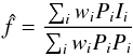 (5)where P is the PSF,
I is the sky-subtracted image, w denotes the pixel
weights in least squares, and the sums run over pixels. The statistically optimal weights
read
(5)where P is the PSF,
I is the sky-subtracted image, w denotes the pixel
weights in least squares, and the sums run over pixels. The statistically optimal weights
read ![Mathematical equation: \hbox{$w_i^{-1}=\mathrm{Var}[I_i] = \mathrm{Var}[{\rm sky}]+k f P_i$}](/articles/aa/full_html/2013/09/aa21668-13/aa21668-13-eq40.png) , where k is the ratio of
a pixel content to its shot noise variance, usually the inverse of the gain. For a faint
source,
, where k is the ratio of
a pixel content to its shot noise variance, usually the inverse of the gain. For a faint
source,  and for a bright source
  ,
so that the relative weights of image pixels
Ii vary with source brightness. Flux ratios
are then accurate only if the PSF model is faithful. Setting
,
so that the relative weights of image pixels
Ii vary with source brightness. Flux ratios
are then accurate only if the PSF model is faithful. Setting
![Mathematical equation: \hbox{$w_i^{-1} = \mathrm{Var}[{\rm sky}]$}](/articles/aa/full_html/2013/09/aa21668-13/aa21668-13-eq44.png) preserves the statistical optimality for
faint sources and makes flux ratios independent of the accuracy of the PSF model, at the
expense of a suboptimal flux estimator for brighter sources. Since the flux ratio
uncertainty is dominated by the uncertainty of the fainter source, and we have several
tertiary stars for each SN, we settled for for both the photometry
of SNe and tertiaries. Note that the reason for assuming a stationary noise when
estimating Gaussian second moments (Eq. (1)) is essentially the same.
preserves the statistical optimality for
faint sources and makes flux ratios independent of the accuracy of the PSF model, at the
expense of a suboptimal flux estimator for brighter sources. Since the flux ratio
uncertainty is dominated by the uncertainty of the fainter source, and we have several
tertiary stars for each SN, we settled for for both the photometry
of SNe and tertiaries. Note that the reason for assuming a stationary noise when
estimating Gaussian second moments (Eq. (1)) is essentially the same.
We however use the optimal pixel weights (i.e. account for all noise sources including
the object itself) when modeling the PSF (Sect. 3.2),
in order to obtain a PSF model as faithful as possible. It is worth stressing that there
is a systematic difference between using ![Mathematical equation: \hbox{$w_i^{-1}= \mathrm{Var}[{\rm sky}]+k f P_i$}](/articles/aa/full_html/2013/09/aa21668-13/aa21668-13-eq45.png) and
and
![Mathematical equation: \hbox{$w_i^{-1}= \mathrm{Var}[{\rm sky}] + k I_i$}](/articles/aa/full_html/2013/09/aa21668-13/aa21668-13-eq46.png) in expression (5), although these two expressions should agree
on average. With the second expression, the flux estimator becomes seriously non linear
w.r.t pixel values Ii and this leads to
unacceptable flux biases, analogue to the ones described in Humphrey et al. (2009). The PSF modeling yields PSF fluxes of tertiary
stars, but those will not be used for comparison with SNe, because they
rely on flux-dependent weights and are not obtained by enforcing a common position on all
images.
in expression (5), although these two expressions should agree
on average. With the second expression, the flux estimator becomes seriously non linear
w.r.t pixel values Ii and this leads to
unacceptable flux biases, analogue to the ones described in Humphrey et al. (2009). The PSF modeling yields PSF fluxes of tertiary
stars, but those will not be used for comparison with SNe, because they
rely on flux-dependent weights and are not obtained by enforcing a common position on all
images.
4. Overview of SN photometry techniques
Photometry of variable sources is required to build lightcurves. Supernovae are not just like variable stars, because they usually appear in galaxies, which constitute a spatially structured background to the SN light. The classical sky subtraction algorithms assume a spatially smooth background (see e.g. Irwin 1985, and references therein) and hence cannot be used. As most galaxy subtraction schemes, we will rely on images of the field without the supernova acquired either before or well after the explosion. Note that as mentioned above, tertiary stars (i.e. stars surrounding the supernova measured in the same frames) should be measured as well and in such a way that flux ratios are as accurate as possible.
Many approaches have been proposed for this differential photometry problem:
-
Measure fluxes in the same aperture on both “on” and “off” images and subtract those, after a proper flux scaling (e.g. Perlmutter et al. 1999). Surrounding stars are measured using the same aperture photometry on both sets of images (and these fluxes indeed define the flux scales).
-
Register (via resampling) the “off” image to align it on the “on” image (or vice versa), match the PSFs (by application of a convolution kernel to the best-IQ image), flux scale one using stars, subtract images, and measure the SN PSF flux on the subtraction (e.g. Hamuy et al. 1994; Schmidt et al. 1998). Surrounding stars are measured using PSF photometry on un-subtracted frames.
-
From the image series, compute all flux differences using the above method. There are N(N-1)/2 such differences and the method is called NN2 (Barris et al. 2005). From this potentially large number of differences, one fits for the actual lightcurve points by least squares, imposing a null flux constraint. Surrounding stars are directly measured using PSF photometry on unsubtracted frames.
-
Fitting a time-independent pixellized galaxy model and a time-variable point source to the image series, forcing the flux to zero in images where the SN is “off”. Surrounding stars are measured using the same technique without fitting a galaxy and without “off” periods (Fabbro 2001; Astier et al. 2006; Holtzman et al. 2008; Guy et al. 2010).
The last approach directly fits the model to the whole data set and might be optimal from a statistical point of view by reaching the minimum variance bound set by the Cramér-Rao inequality. The NN2 technique could reach statistical optimality if it tracked the covariance of all flux differences when computing the actual lightcurve. The method is however computationally prohibitive when dealing with several hundred images. The technique sketched in point 2 above approaches statistical optimality because there is not much information to gain about the galaxy light distribution under the SN from images with the SN. By not using PSF photometry, the method 1 is suboptimal from a statistical point of view, but independent of any PSF modeling, at variance with all other approaches. Method 1 also does not require image resampling, at variance with methods 2 and 3.
This paper will discuss two incarnations of the full model technique (method 4 above): one method assumes that all images are on the same pixel grid and hence requires resampled images, and the other resamples the model rather than the input data, as originally proposed in Holtzman et al. (2008). In both instances, we use the weighting scheme discussed in Sect. 3.3 which avoids the shortcomings of inaccurate PSF modeling.
5. Resampled simultaneous photometry (RSP)
The first step of the resampled simultaneous photometry (RSP) consists in identifying the best IQ image of the series (“the reference”), and resample all other images to the same pixel grid as this image. The needed geometrical mappings are fitted to the catalogs and leave residuals typically around 0.15 pixel (dominated by shot noise). Note that we also resample the weight maps, in particular to properly account for pixels with null weight. Then, discrete convolution kernels are fitted to the aligned image pairs in order to match the PSF of the reference to all the other images of the series, using the Alard & Lupton (1998) algorithm. More precisely, we fit a spatially variable kernel (Alard 2000), which can compensate minor misalignment residuals, and we impose a position-independent kernel integral. The fit is carried out on stamps centered on the 150 (non-saturated) objects in the frame with the highest peak flux. Note that the fitted kernel matches both the PSF shape and the flux scale of the involved image pair.
On the set of aligned images, the model for the expected light in image i
at pixel p reads: ![Mathematical equation: \begin{equation} M_{i,p} = \left \{ \left [ f_i \times \phi_{\rm ref} ({\boldsymbol x_p} - {\boldsymbol x_{\rm SN}} ) + gal_{\rm ref} \right ] \otimes K_i \right \}_p +s_i \label{eq:light_model} \end{equation}](/articles/aa/full_html/2013/09/aa21668-13/aa21668-13-eq48.png) (6)where
fi is the SN flux in image
i, galref is the galaxy pixel
map in the reference image (assumed to be non-variable in time) at the sampling of this
reference image, Ki is the convolution kernel
to match the reference image PSF φref and flux scale to the ones
of image i. si is the sky of
image i. This model is compared to data using least squares:
(6)where
fi is the SN flux in image
i, galref is the galaxy pixel
map in the reference image (assumed to be non-variable in time) at the sampling of this
reference image, Ki is the convolution kernel
to match the reference image PSF φref and flux scale to the ones
of image i. si is the sky of
image i. This model is compared to data using least squares:
 (7)where
Ii,p is the data. The fit parameters are
one flux per “on” image, a single SN position, the galaxy pixel map, and a sky level per
image, except for one image, because it would be degenerate with a spatially-constant flux
added to the galaxy map3. We only fit a stamp around
the SN, typically of 10 times σIQ on a side. Convolution kernels
are also pixel maps whose size is adjusted to the IQ difference they are expected to bridge.
The galaxy map is fitted up to the size required by the worst IQ image in the series,
typically 50 pixels on a side.
(7)where
Ii,p is the data. The fit parameters are
one flux per “on” image, a single SN position, the galaxy pixel map, and a sky level per
image, except for one image, because it would be degenerate with a spatially-constant flux
added to the galaxy map3. We only fit a stamp around
the SN, typically of 10 times σIQ on a side. Convolution kernels
are also pixel maps whose size is adjusted to the IQ difference they are expected to bridge.
The galaxy map is fitted up to the size required by the worst IQ image in the series,
typically 50 pixels on a side.
When fitting a supernova, we impose fi = 0 on images acquired before or long after the explosion. When fitting the lightcurve of a tertiary star, we impose that the underlying galaxy galref is zero, and also allow sky level si to vary in all images (as opposed to freezing one to zero when fitting the galaxy).
One might note that the fit assumes pixels to be independent, thus ignoring the correlations introduced between neighbouring pixels by resampling, because the latter are not easily tractable. For linear least squares, approximating the uncertainties is not a source of bias, but is suboptimal, as stated by the Gauss-Markov theorem4. Because the object’s position does not enter linearly in the fit, the argument does not strictly apply and we will discuss shortly realistic simulations that may detect a possible flux bias. Regarding optimality, simplified simulations show that ignoring correlations due to resampling when measuring PSF fluxes on resampled images has a negligible effect on the real variance of the flux estimator, for the typical spatial sampling we are considering here. Because resampling introduces mostly positive correlations between neighbouring pixels, the flux variance estimated from propagating the apparent sky variance is usually underestimated.
6. Direct simultaneous photometry (DSP)
The direct simultaneous photometry (DSP) aims at avoiding any resampling of the data. Since input pixels are then uncorrelated, ignoring correlations is no longer an approximation. Propagation of the shot noise is tractable, and one saves the computer mass storage corresponding to resampled images. The method can be used on under-sampled images (fitting an over-sampled galaxy model). The tests presented in Sect. 7 are more complete than for the RSP method.
The DSP method requires a PSF model for each image in the series, and coordinate transformations that map images one on the other. We have already discussed the production of the PSF of each image in Sect. 3.2, and we will first describe how we obtain the necessary coordinate mappings. We then discuss atmospheric refraction and star positions because position variations matter for fluxes in the context of a fit that imposes a common position on all images. We eventually describe the fit itself.
6.1. Relative astrometry of the image series
Since we are fitting SNe simultaneously to an image series, imposing a fixed position on the sky, we have to transform its position (in some frame) into pixel coordinates in any image of the series. Since we are going to use these transformations to position a PSF on each image, these transformations should be determined using coordinates obtained using the same PSF model as the one that will be used during the fit. We hence adjust transformations using PSF-fitted coordinates of stars, which are a by-product of PSF modeling (Sect. 3.2).
Our image series consists in all images from a given CCD, gathered in exposures of one of
our fields in a given band. These images are equipped with a WCS accurate to better than 1
pixel, which can be used to associate all stars detected in the image series. We typically
have ~200 stars, with a total of  measurements. Because of saturation, the brightest stars are only usable on the poorest IQ
images, while the faintest ones can only be measured on the best IQ images. For the star
i, its expected position
Pij in image
j is modeled as
measurements. Because of saturation, the brightest stars are only usable on the poorest IQ
images, while the faintest ones can only be measured on the best IQ images. For the star
i, its expected position
Pij in image
j is modeled as  (8)where
Tj is the coordinate mapping from a
reference system to pixels in image j,
Xi refers to the coordinates
of star i in this reference system,
μi the proper motion of this
star, tj the epoch of image
j and t0 some reference epoch. The
parameters of the astrometric fit are Tj (one
per image), Xi and
μi (one position and one
proper motion per star). We choose the best IQ image as the reference system: its
transformation T is just the identity and is not fitted. We choose the
reference epoch t0 as the mean survey epoch. The
transformations T are modeled as polynomial functions of the
cooordinates5, and we chose quadratic functions
because a higher degree did not seem to improve significantly the residuals. Conversely,
linear transformations increase the rms residuals by a factor of 2 to 3 with respect to
quadratic ones. Note that these transformations map images from the same intrument on each
other, and coordinate mappings from CCD coordinates to the sidereal coordinates do require
higher orders.
(8)where
Tj is the coordinate mapping from a
reference system to pixels in image j,
Xi refers to the coordinates
of star i in this reference system,
μi the proper motion of this
star, tj the epoch of image
j and t0 some reference epoch. The
parameters of the astrometric fit are Tj (one
per image), Xi and
μi (one position and one
proper motion per star). We choose the best IQ image as the reference system: its
transformation T is just the identity and is not fitted. We choose the
reference epoch t0 as the mean survey epoch. The
transformations T are modeled as polynomial functions of the
cooordinates5, and we chose quadratic functions
because a higher degree did not seem to improve significantly the residuals. Conversely,
linear transformations increase the rms residuals by a factor of 2 to 3 with respect to
quadratic ones. Note that these transformations map images from the same intrument on each
other, and coordinate mappings from CCD coordinates to the sidereal coordinates do require
higher orders.
The model is almost degenerate: if one operates the substitutions:
 where g is any arbitrary
function, the predicted position is not changed if the transformations
Tj are linear, which happens to be almost
exactly true. Non-moving objects obviously lift the degeneracy, and inserting galaxies
into the fit seems an obvious cure. However, the position of galaxies with respect to
stars depends on the chosen definition of position, and are likely to depend on details of
the PSF. We hence resorted to iteratively isolating a subset of stars affected by proper
motions: all stars are initially fixed, and we release at most one star per iteration,
requiring that its release decreases its contribution to the
χ2 by a factor of 2 or more. We also allow each iteration to
discard a small number of outlier measurements. The fit stops when no star status was
changed (fixed or allowed to move) nor any measurement was discarded.
where g is any arbitrary
function, the predicted position is not changed if the transformations
Tj are linear, which happens to be almost
exactly true. Non-moving objects obviously lift the degeneracy, and inserting galaxies
into the fit seems an obvious cure. However, the position of galaxies with respect to
stars depends on the chosen definition of position, and are likely to depend on details of
the PSF. We hence resorted to iteratively isolating a subset of stars affected by proper
motions: all stars are initially fixed, and we release at most one star per iteration,
requiring that its release decreases its contribution to the
χ2 by a factor of 2 or more. We also allow each iteration to
discard a small number of outlier measurements. The fit stops when no star status was
changed (fixed or allowed to move) nor any measurement was discarded.
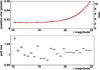 |
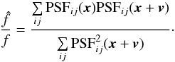
Fig. 2 Astrometric 1D residuals scatter as a function of star magnitude for the D3 field in r band. The top plot compares, as a function of magnitude, the measured residual rms (points) with the average expected rms (curve) including a noise floor of 0.013 pixels. They are roughly compatible, but not necessarily equal because the expected rms varies with IQ at fixed magnitude. The bottom plot displays the rms of the residual pulls (i.e. residuals in unit of expected rms), which are close to 1 at all magnitudes. We hence conclude that adding the position noise floor of 0.013 pixels (2.4 mas) in quadrature to the position uncertainty expected from shot noise fairly describes the residuals. This figure only considers residuals along y for reasons explained in Sect. 6.2. |
We initially used the position uncertainties from PSF position measurements (i.e. propagation of shot noise), but those proved to be inadequate at the bright end, where they possibly reach 0.002 pixel rms. We hence added in quadrature a “position noise floor” of 0.013 pixels rms, adjusted to the residuals at the bright end. Figure 2 illustrates that this simple uncertainty model adequately describes the observed scatter. We find similar noise floor values for all bands. This astrometric noise floor of 0.013 pixel or 2.4 mas is significantly better than the one reported for wide-field ground-based astrometry in Anderson et al. (2006). In contrast, Lazorenko (2006) obtains a significantly better result than ours, but on a narrower field instrument.
Although the astrometric precision has a negligible influence on the quality of our photometric measurements, we searched for systematic errors contributing to the astrometric precision floor, and we report one related serendipitous finding (which does not explain the observed residual) in Appendix B.
The precision of proper motion measurements can be assessed by comparing the proper motions detected in two different bands, because the fits are performed independently. Comparing non-zero proper motions in r and i bands, we find rms differences of ~1.5 mas/y per coordinate, indicating a precision of ~1 mas/y in each band. This figure is about 5 times worse than anticipated from the single-image astrometric precision of ~7 mas, and we attribute most of this difference to our crude algorithm used to separate fixed and moving stars, which does not aim at optimizing proper motion measurements. Optimizing the proper motion precision would also likely benefit from accounting for atmospheric refraction (that we discuss in next paragraph) as well as pixel size discontinuities (discussed in Appendix B). Note that the influence of proper motion inaccuracies on geometrical transformations are indeed tested by the simulations described in Sect. 7.
6.2. Position shifts induced by atmospheric refraction
This section justifies why we can ignore the effect of atmospheric refraction when
mapping coordinates of different images. Atmospheric refraction bends light rays in a
plane that contains the incoming direction and the vertical at the observatory. Light rays
from zenith are unaffected. This bending displaces the objects in the image plane:
![Mathematical equation: \begin{eqnarray} \label{eq:deltax}&&\delta x = [n(\lambda)-1] \tan z \sin \eta \\ \label{eq:deltay}&&\delta y = [n(\lambda)-1] \tan z \cos \eta \end{eqnarray}](/articles/aa/full_html/2013/09/aa21668-13/aa21668-13-eq71.png) where n(λ)
is the refraction index of the atmosphere, z is the zenith angle and
η is the parallactic angle, the direction of the refraction-induced
displacement in the image plane. We recall that with MegaCam, x and
y are well aligned with right ascension and declination. The law of
sines relates the parallactic angle with other angles describing the observing conditions:
where n(λ)
is the refraction index of the atmosphere, z is the zenith angle and
η is the parallactic angle, the direction of the refraction-induced
displacement in the image plane. We recall that with MegaCam, x and
y are well aligned with right ascension and declination. The law of
sines relates the parallactic angle with other angles describing the observing conditions:
 (11)where ℓ is the latitude of
the observatory and h is the hour angle, i.e. the RA difference between
the target and the zenith. Atmospheric refraction displaces the whole image (by
~30−40′′ in the visible, for tanz = 1, on the Mauna Kea), with a
small distortion due to the variation of zenith angle across the field of view. Both
effects are absorbed into the geometrical transformations (Eq. (8)). Conversely, we are sensitive to the
different displacement of wavelengths within the observing band, which is oriented in the
same direction as the total displacement and scales with the difference of refractive
indices between cuton and cutoff wavelengths of the band. As a consequence,
g is the most affected band. This differential displacement moves red
and blue stars in opposite directions w.r.t. an average-color star, and we are only
sensitive to the scatter of these displacements across images, which scales with the
scatter of tanzsinη and
tanzcosη along x and
y respectively. It turns out that
σ(tanzsinη) ~0.4, and
σ(tanzcosη) is typically 10 times
smaller (see Table 3). This is a consequence of our
observing the science fields over as long a season as possible, and we will concentrate in
the following discussion on the x coordinate, the most affected one. We
choose to index star colors by g − i, and, assuming
their spectra to be power laws, we can approximate the displacement of a star in a given
image with respect to its average position as:
(11)where ℓ is the latitude of
the observatory and h is the hour angle, i.e. the RA difference between
the target and the zenith. Atmospheric refraction displaces the whole image (by
~30−40′′ in the visible, for tanz = 1, on the Mauna Kea), with a
small distortion due to the variation of zenith angle across the field of view. Both
effects are absorbed into the geometrical transformations (Eq. (8)). Conversely, we are sensitive to the
different displacement of wavelengths within the observing band, which is oriented in the
same direction as the total displacement and scales with the difference of refractive
indices between cuton and cutoff wavelengths of the band. As a consequence,
g is the most affected band. This differential displacement moves red
and blue stars in opposite directions w.r.t. an average-color star, and we are only
sensitive to the scatter of these displacements across images, which scales with the
scatter of tanzsinη and
tanzcosη along x and
y respectively. It turns out that
σ(tanzsinη) ~0.4, and
σ(tanzcosη) is typically 10 times
smaller (see Table 3). This is a consequence of our
observing the science fields over as long a season as possible, and we will concentrate in
the following discussion on the x coordinate, the most affected one. We
choose to index star colors by g − i, and, assuming
their spectra to be power laws, we can approximate the displacement of a star in a given
image with respect to its average position as:  (12)where
kf is a constant depending on the
considered filter f, and
g − i − ⟨g − i⟩
is the difference in color of this star to the average color of the stars involved in the
astrometric fit. We have assumed in Eq. (12) that ⟨tanzsinη⟩ ~ 0, which is
fairly accurate for a survey such as SNLS (see Table 3), and Fig. 3 illustrates that this
expression (12) describes a detectable
effect. We measure kg ≃ 0.13 pixels from this figure and
computations using the Pickles (1998) stellar
library yield a similar value for the typical Mauna Kea air column.
(12)where
kf is a constant depending on the
considered filter f, and
g − i − ⟨g − i⟩
is the difference in color of this star to the average color of the stars involved in the
astrometric fit. We have assumed in Eq. (12) that ⟨tanzsinη⟩ ~ 0, which is
fairly accurate for a survey such as SNLS (see Table 3), and Fig. 3 illustrates that this
expression (12) describes a detectable
effect. We measure kg ≃ 0.13 pixels from this figure and
computations using the Pickles (1998) stellar
library yield a similar value for the typical Mauna Kea air column.
We evaluate the color spread of stars involved in the fit to σ(g − i) ≃ 0.9. In the SNLS, we typically have σ(tanzsinη) ≃ 0.4, so that refraction contributes σ(δx) ≃ 0.9 × 0.4 × 0.13 = 0.047 pixels to astrometric residuals along x for g band, compatible to ~10% with the difference in scatter between residuals along x (0.057 pixels) and y (0.026 pixels).
We have considered incorporating differential refraction into the astrometric model (Eq. (8)). As for proper motions, we would then have to account for the star displacements induced by refraction when carrying out the simultaneous photometry fit. Our insistance on treating SNe and tertiaries as similarly as possible would then face a problem: predicting the displacement requires a color, SN colors vary with phase and we do not have color measurements at all phases. More fundamentally, setting up a photometry scheme that relies on the colors of the object we are trying to measure is not very appealing. The alternative is to just ignore refraction for both stars and SNe, and we will now evaluate the incurred loss of photometric accuracy.
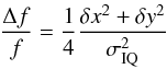
We now evaluate the effect of displacements induced by refraction on the ratio of SN flux
fSN to tertiary star flux f∗,
using expression (3), and averaging over
tertiaries. We have: ![Mathematical equation: \begin{eqnarray} \frac{\delta E \left[ f_{\rm SN}/f_* \right]}{ E \left[ f_{\rm SN}/f_* \right]} & =& \frac{\delta f_{\rm SN}}{f_{\rm SN}} - E \left[ \frac{\delta f_{*}}{f_{*}} \right] \nonumber \\[1.5mm] &=& \frac{1}{4} \frac{ (\delta x_{\rm SN})^2 - E [(\delta x_*)^2]}{ \sigma_{\rm IQ}^2} \nonumber \\[1.5mm] & =& k_{\rm g}^2 \frac{(c_{\rm SN} - \bar{c})^2 - Var (c_*)}{ 4 \sigma_{\rm IQ}^2} \mathrm{Var}[ \tan z \sin \eta ] \nonumber \\[1.5mm] && \simeq 1.5\ 10^{-4} \left[(c_{\rm SN} - \bar{c})^2 - 0.7 \right] \end{eqnarray}](/articles/aa/full_html/2013/09/aa21668-13/aa21668-13-eq96.png) (13)where c denotes
g − i,
(13)where c denotes
g − i,  the average over stars, and we have assumed σIQ = 2. We see
that in order to bias flux ratios by more than one part in thousand, the color of the SN
would need to be 3 mag different from the average star. This is not the case for SNe Ia at
the redshifts we are considering, and such sources are very rare. Would the algorithm have
to cope with such an odd source, one could still incorporate the displacement induced by
refraction into the model. For “regular” sources, and in particular SNe Ia, it is in fact
more favorable (and obviously simpler) to just ignore atmospheric refraction, which will
be our line of conduct in what follows.
the average over stars, and we have assumed σIQ = 2. We see
that in order to bias flux ratios by more than one part in thousand, the color of the SN
would need to be 3 mag different from the average star. This is not the case for SNe Ia at
the redshifts we are considering, and such sources are very rare. Would the algorithm have
to cope with such an odd source, one could still incorporate the displacement induced by
refraction into the model. For “regular” sources, and in particular SNe Ia, it is in fact
more favorable (and obviously simpler) to just ignore atmospheric refraction, which will
be our line of conduct in what follows.
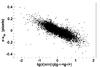 |
Fig. 3 Astrometric residuals along x (i.e. RA) in g band as a function of the displacement expected from refraction, up to an unknown constant, for stars brighter than i = 20. |
6.3. Photometric fit
The DSP algorithm discussed in this section does not resample the images, but instead
resamples the model, so that the data pixels to which the model is compared are indeed
independent, and diagonal least squares are not an approximation. The statistical benefit
in terms of photometric noise turns out to be small in our case because MegaCam images are
well sampled. Note that for poorly sampled images, avoiding resampling becomes essentially
mandatory for precision work. The flux expected for image i at pixel
p (located at
xp), reads: ![Mathematical equation: \begin{equation} M_{i,p} = \left [f_i \times \phi_i({\boldsymbol x_p}-T_i[{\boldsymbol x_{\rm obj}}]) + G\left(T_i^{-1}({\boldsymbol x_p})\right) \otimes K_i + S_i \right ] R_i \label{eq:DSP-model} \end{equation}](/articles/aa/full_html/2013/09/aa21668-13/aa21668-13-eq102.png) (14)where
fi is the object flux in image
i, φi the PSF function in
the same image, Ti is the geometrical
transformation to the reference image (defined in Eq. (8)), G is the galaxy pixelized model for the PSF of
the reference image, and Ki the convolution
kernel that matches the PSF of the reference to the one of image i (at
the object position), Si is the sky level in
image i, Ri the photometric
ratio of the reference to image i, and
xobj is the coordinate of the object (in the
reference frame). fi, G,
Si and
xobj are the fit parameters. The kernels
Ki are fitted from the PSFs of the
reference image and the image i, and has to be multiplied by the
photometric ratio of the same images, fitted from the PSF fluxes, a by-product of PSF
modeling (Sect. 3.2). Modeling uniform photometric
ratios over a CCD seems adequate because we have found a high correlation of photometric
ratios of different CCDs within an exposure. This approximation does not cause flux biases
but only contributes a small additional random error, bounded by the reproducibility of
bright star fluxes, i.e. ~0.006 mag (Sect. 7.5.3).
(14)where
fi is the object flux in image
i, φi the PSF function in
the same image, Ti is the geometrical
transformation to the reference image (defined in Eq. (8)), G is the galaxy pixelized model for the PSF of
the reference image, and Ki the convolution
kernel that matches the PSF of the reference to the one of image i (at
the object position), Si is the sky level in
image i, Ri the photometric
ratio of the reference to image i, and
xobj is the coordinate of the object (in the
reference frame). fi, G,
Si and
xobj are the fit parameters. The kernels
Ki are fitted from the PSFs of the
reference image and the image i, and has to be multiplied by the
photometric ratio of the same images, fitted from the PSF fluxes, a by-product of PSF
modeling (Sect. 3.2). Modeling uniform photometric
ratios over a CCD seems adequate because we have found a high correlation of photometric
ratios of different CCDs within an exposure. This approximation does not cause flux biases
but only contributes a small additional random error, bounded by the reproducibility of
bright star fluxes, i.e. ~0.006 mag (Sect. 7.5.3).
The galaxy model G is by default modeled at the same sampling as the input images, although one can consider a finer sampling. As written above, Megacam images are well sampled (FWHM > 4 pixels on average), so that resampling does not significantly smooth the sharpest objects. One might be concerned because the galaxy is modeled at the best IQ of the image series, and the shortcomings of resampling under-sampled images might be at play. It turns out that in expression (14), the galaxy model G is smoothed by a convolution kernel. We hence resample a galaxy model with the same IQ as the used images, which are on average well sampled. We note that the simulations we describe below to test the DSP method could indeed detect a bias induced by resampling, in particular by looking for photometric residuals varying with IQ, and found none.
For the fit of tertiaries, the galaxy part of the model is set to zero, and the position in each image xobj,i = xobj + μobj(ti − tref) accounts for proper motion μobj when applicable.
6.3.1. Fitting all bands simultaneously?
Readers might wonder why we process pass-bands independently, since enforcing common values of nuisance parameters (e.g. star positions, proper motions) usually reduces random errors of parameters of interest (e.g. SN and star fluxes). Fitting the astrometry in all bands simultaneously would reduce the uncertainty of output catalogs, provided the impact of atmospheric refraction remains small (note that Sect. 6.2 only discusses refraction-induced offsets between images from the same band, not offsets between different bands). However, the photometric fit does not use positions from the astrometric fit, but only uses the fitted proper motions and transformations. The uncertainties of the proper motions are too small to compromise the photometric accuracy. Improving the fitted catalog will marginally improve the fitted transformations, since their uncertainties mostly result from position measurement uncertainties in the image they are mapping.
Regarding the simultaneous photometric fit itself, fitting jointly all bands would improve the quality of positions, which does not reduce the variance of fluxes but instead reduces the bias of flux estimators at low S/N (see Sect. 3.3). For SNLS, this last point is only relevant in practice for distant supernovae, which may exhibit low S/N in g and z bands. Conversely, all supernovae have a large enough integrated S/N in r and i bands. We hence fit supernovae in g and z bands at a fixed position, provided by r and i bands, and study the possible shortcomings of the procedure in Sect. 9.2.
Since the benefits of fitting all bands simultaneously are at best tenuous, and might require a proper accounting of refraction, we did not attempt it.
6.3.2. Dealing with the Poisson noise from objects
As discussed in Sect. 3.3, we deliberately ignore
the contribution of the objects to the noise when estimating fluxes, in order to ensure
linearity, independently of the fidelity of the PSF. As a consequence, the flux
uncertainties obtained from the second derivatives of the χ2
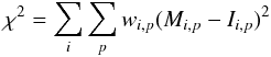
at minimum are underestimated. The parameters, and their actual uncertainties read:
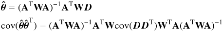 (15)with
χ2 = (Aθ − D)TW(Aθ − D),
and:
(15)with
χ2 = (Aθ − D)TW(Aθ − D),
and:
-
W is the weight matrix actually used in the fit.
-
D is the data vector.
-
θ is the vector containing the model parameters.
-
A is the design matrix, i.e. E [D] = Aθ.
In standard least squares, we would have
W-1 = cov(DDT), and
 ,
which is the minimum variance bound. For reasons discussed in Sect. 3.3, we choose pixel weights
,
which is the minimum variance bound. For reasons discussed in Sect. 3.3, we choose pixel weights  . This choice leads to a suboptimal fit,
as indicated by the Gauss-Markov theorem, but we find that the loss in precision is
insignificant. Indeed, the simulations that follow indicate an average increase of
uncertainties around 2.5% above the minimum variance bound for typical tertiary stars.
. This choice leads to a suboptimal fit,
as indicated by the Gauss-Markov theorem, but we find that the loss in precision is
insignificant. Indeed, the simulations that follow indicate an average increase of
uncertainties around 2.5% above the minimum variance bound for typical tertiary stars.
7. Validations with simulations
7.1. Simulation goals
The fundamental requirement of SN photometry is the preservation of flux ratios between field stars and SN. We therefore designed a simulation whose aim is to ensure that this ratio is maintained across a wide range of photometric conditions. In particular we want to ensure that:
-
fitting a galaxy model during SN photometry does not induce anybiases. Indeed, galaxy fitting is the only algorithmic differencebetween SN and tertiary/calibration star photometry;
-
flux ratios are properly recovered over a wide enough range of IQ and S/N;
-
after tuning some aspects of the uncertainty model, it properly describes the observed scatter;
-
sampling the galaxy model at the same spatial sampling as the images is fine enough.
7.2. Simulation method
The simulation consists in modifying real SNLS science images by adding so called fake stars to them. These fake stars are constructed by copying and pasting image stamps of bright, high photometric quality stars, dubbed model stars, onto a nearby galaxy after being appropriately dimmed. We translate the model star by an integer number of pixels before pasting, thus avoiding any shortcomings of resampling. Note also that the time window during which the fake SN is turned on is randomly selected. At variance with many proposed tests of SN photometry (e.g. Schmidt et al. 1998; Holtzman et al. 2008), this copy-paste method is independent of PSF modeling, astrometric mappings, and photometric ratios between images, and hence might detect the effects of improper estimates of these inputs.
The idea, then, is to test a photometry by its ability to reproduce the photometric
factor used to dim the model star. To construct a lightcurve for each model and fake star
pairing, the same procedure is applied for each pair on a set of images. As the RSP
photometry runs on aligned images, one can translate the pixels of the model star by the
same amount on all images and is guaranteed to always land on the same position on the
sky. For the DSP photometry, this is clearly not the case, and we must be careful to
select unaligned (and therefore un-resampled) images that are, by sheer happenstance, very
nearly aligned up to a translation. The underestimation of the flux as a result of a
position error, for a Gaussian PSF, is given by Eq. (3). Given a rotation between 2 images of angle Δθ, a
relative difference in plate scale noted Δλ/λ and a
displacement vector v between the model and fake star, Eq.
(3) can be rewritten as: ![Mathematical equation: \begin{equation} \frac{\Delta f}{f} = \frac{1}{4} \left( \frac{||\boldsymbol{v}||}{\sigma _{\rm seeing}} \right)^2 [(\Delta \theta)^2 + (\Delta \lambda / \lambda)^2]. \label{eq:deltaFWCS} \end{equation}](/articles/aa/full_html/2013/09/aa21668-13/aa21668-13-eq124.png) (16)We use Eq. (16) to select bunches of consecutive images such that they yield a
difference in flux under the 10-3 level if
| |v|| = 100 pixels. Fake stars constructed with a larger
value for | |v| | are not considered in the analysis. We
indeed find un-rotated successive image bunches because CFHT enjoys an equatorial mount
and the camera (which has no rotation capability) is usually mounted on its top end once
for a whole dark-time run. The fake stars are only pasted during these lunations, leaving
their flux at 0 for the remaining images, thereby simulating top-hat lightcurves for these
fake “supernovae”. Note that to avoid correlations, we only cut and paste one fake star
per galaxy per lunation. For this simulation, we use r-band images in CCD 13 of field D1,
in CCD 11 of field D2, and in CCD 12 of field D4. The chosen CCDs are near the center of
the CCD mosaic.
(16)We use Eq. (16) to select bunches of consecutive images such that they yield a
difference in flux under the 10-3 level if
| |v|| = 100 pixels. Fake stars constructed with a larger
value for | |v| | are not considered in the analysis. We
indeed find un-rotated successive image bunches because CFHT enjoys an equatorial mount
and the camera (which has no rotation capability) is usually mounted on its top end once
for a whole dark-time run. The fake stars are only pasted during these lunations, leaving
their flux at 0 for the remaining images, thereby simulating top-hat lightcurves for these
fake “supernovae”. Note that to avoid correlations, we only cut and paste one fake star
per galaxy per lunation. For this simulation, we use r-band images in CCD 13 of field D1,
in CCD 11 of field D2, and in CCD 12 of field D4. The chosen CCDs are near the center of
the CCD mosaic.
7.3. Expected biases
7.3.1. PSF spatial variation bias
We expect a small simulation-induced bias as a function of displacement from model to
fake star due to variations in the PSF as we move across the image. Indeed, the fake
star generation process cuts a star with a given PSF and pastes it in a location where
the PSF is slightly different. The induced bias as a result of this is given by:
 (17)Because the change in the PSF model is
linear by construction with respect to position in an image, expression (17) depends linearly on
v. To directly observe this bias, we run simulations
with a photometric ratio of 1 and avoid adding Poisson noise. We also compute the
expected trend using Eq. (17) for a wide
range of v summed across all images used during the
simulation. The trend expected by direct computation matches the one observed for
simulations, and the effect is clearly linear in v. This
bias is well below the 10-3 level for typical v
used during the simulation. Furthermore, the bias disappears when one averages over
v directions. We hence did not take any action to
account for the PSF variation from model to fake star positions in our simulations.
(17)Because the change in the PSF model is
linear by construction with respect to position in an image, expression (17) depends linearly on
v. To directly observe this bias, we run simulations
with a photometric ratio of 1 and avoid adding Poisson noise. We also compute the
expected trend using Eq. (17) for a wide
range of v summed across all images used during the
simulation. The trend expected by direct computation matches the one observed for
simulations, and the effect is clearly linear in v. This
bias is well below the 10-3 level for typical v
used during the simulation. Furthermore, the bias disappears when one averages over
v directions. We hence did not take any action to
account for the PSF variation from model to fake star positions in our simulations.
7.3.2. Low S/N bias
We have seen in Sect. 3.3 that PSF flux measurements are biased at low S/N, due to position uncertainties. When a common position is fitted for a source in an image series, the bias is lower but does not disappear.
For a flux measurement on a single image i of flux
fi, the S/N is defined simply as the
ratio of fi to
 . For a light-curve of any shape, the
least-squares estimator of its amplitude A has a variance that satisfies:
. For a light-curve of any shape, the
least-squares estimator of its amplitude A has a variance that satisfies:
![Mathematical equation: \begin{equation} \frac{{\bf A}^2}{\mathrm{Var}[\bf\hat{A}]} = \Sum{i}{} \frac{f_i^2}{\mathrm{Var}[\hat{f_i}]} \label{eq:globalSN} \end{equation}](/articles/aa/full_html/2013/09/aa21668-13/aa21668-13-eq130.png) (18)where
fi is the expected flux in each image.
(18)where
fi is the expected flux in each image.
In Appendix B of Guy et al. (2010), it is shown
that the bias of  follows the same law as for a single image (described in
Eq. (4)), namely: ![Mathematical equation: \begin{equation} \frac{{E}[\bf\widehat{A}]}{\bf A} \simeq \left\{ 1 - \frac{\mathrm{Var}[\bf\widehat{A}]}{A^2} \right\} \cdot \label{eq:amp-bias} \end{equation}](/articles/aa/full_html/2013/09/aa21668-13/aa21668-13-eq132.png) (19)For the noisiest supernova observed, this
is expected to correspond to a bias of a few parts in a thousand. To make precision
tests of the photometric accuracy at low S/N we need to take into account this bias. The
photometry’s ability to reconstruct the photometric ratio will therefore be tested as a
function of its S/N, as defined in Eq. (18). To detect any remaining bias, we fit Eq. (19) with an additional constant offset term b:
(19)For the noisiest supernova observed, this
is expected to correspond to a bias of a few parts in a thousand. To make precision
tests of the photometric accuracy at low S/N we need to take into account this bias. The
photometry’s ability to reconstruct the photometric ratio will therefore be tested as a
function of its S/N, as defined in Eq. (18). To detect any remaining bias, we fit Eq. (19) with an additional constant offset term b:
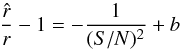 (20)where r the flux ratio
used during the cut and paste,
(20)where r the flux ratio
used during the cut and paste,  the reconstructed flux ratio, and b is a free parameter.
7.3.3. Model star correlations
Because the same model star is reused in multiple model fake star pairing, we take into account possible correlations induced by this repetition and their impact on the simulation’s precision. To do this, we increase the uncertainty on the model star flux until the χ2 per degree of freedom becomes 1 when fitting Eq. (20). We find that we must add 1% uncertainty to the DSP fluxes of the model star, and 0.8% to the RSP fluxes.
7.4. Simulation parameters
We compare the fake star’s simulated parameters with those of real SN, measured during
the SNLS 3-year analysis in order to ensure that the simulation tests the photometry in a
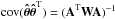
wide range of realistic conditions. In Fig. 4 we show
density plots in the plane of the ratio of the galaxy flux to the SN flux as a function of
the supernova S/N for both real data and the simulation. The galaxy flux is defined as the
integral of the galactic flux weighted by the PSF. For a galaxy model
G(i,j), this is computed as: 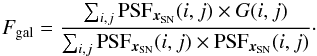 (21)With this comparison, we see that the
distribution of simulated parameters resembles that of real data, however with more galaxy
flux on average in simulations than in real data. This helps at detecting possible
shortcomings of fitting a structured galaxy. We recall that the images used during fake
star photometry are the same as those used for SNLS science photometry, and we can
therefore be confident that the simulation closely mimics the observing conditions of SN
photometry.
(21)With this comparison, we see that the
distribution of simulated parameters resembles that of real data, however with more galaxy
flux on average in simulations than in real data. This helps at detecting possible
shortcomings of fitting a structured galaxy. We recall that the images used during fake
star photometry are the same as those used for SNLS science photometry, and we can
therefore be confident that the simulation closely mimics the observing conditions of SN
photometry.
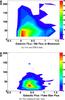 |
Fig. 4 Above are density plots comparing the distribution of real SN and simulated fake stars in the plane of galactic flux vs. S/N. |
In addition to selection factors that are aimed at mimicking the SN population, we perform cuts necessary for proper analysis of the simulation results. A number of model stars used turned out to be variable stars. These are cut from the analysis. We also cut all fake stars generated using a photometric factor above 0.1 so that the original Poisson noise of the model star becomes negligible compared to that added to the fake star during the cut and paste. Finally, model stars that are cataloged as having a significant proper motion are also cut, because the DSP photometry will take into account their motion but not that of the corresponding fake SN.
7.5. Results
7.5.1. Photometric accuracy of RSP
We begin by analyzing the results for the RSP. This technique was used for measuring the SNLS supernovae reported in Astier et al. (2006) and Guy et al. (2010). In Fig. 5, we see the result of fitting Eq. (20) to the photometric ratios obtained. We find that this method overestimates the flux of SN by a factor of (1.75 ± 0.83) × 10-3. This bias has not been found to depend on galactic flux, model or fake star flux, star color, or IQ. A number of tests were performed in an attempt to determine its origin. These are:
-
Reducing the vignette size used by RSP. A change would indicatethat pollutions in the vignette are causing the flux bias, but the biasremained.
-
Keeping the photometric factor at 1, and pasting the fake star on a dark patch of sky. We then compare the photometry of the fake star with and without a galaxy fit. A difference would indicate that flux transfers between fitted galaxy and fitted SN are causing the bias. No significant difference was observed.
-
Fitting the flux average of the RSP fake star lightcurve using the covariance matrix produced by DSP, to see if the error model of RSP was biasing. The bias remained.
-
Switching to i band. Again, the bias remained.
We conclude that the measured bias is likely to be a statistical fluctuation of the simulations at the 2σ level. This photometry method was used in particular to produce the SNLS light curves published in Guy et al. (2010), and we recommend adding a correlated 1.75 × 10⁻³ relative systematic uncertainty to this data set, which amounts to less than 1/3 of the photometric calibration uncertainty.
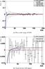 |
Fig. 5 Photometric factor accuracy as a function of S/N for the RSP method. |
7.5.2. Photometric accuracy of DSP
From this section on, the results refer to those obtained using the DSP method. We begin by fitting Eq. (20) to the data. The fit is seen in Fig. 6. We find that no offset exists beyond the 10-3 level. The fitted offset value is (0.12 ± 0.9) × 10-3.
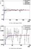 |
Fig. 6 Photometric factor accuracy as a function of S/N for the DSP method. |
Field star and SN photometry differ most crucially in that during the SN fit we also fit a galaxy model. We therefore also investigate photometric accuracy as a function of galactic flux, as defined in Eq. (21). In Fig. 7 we look at the evolution of photometric accuracy as a function of galactic flux after we have corrected for the S/N bias. No significant remaining bias is observed.
Finally, we also find that preservation of flux ratios does not vary with image quality, as shown in Fig. 8. Again, the S/N bias is corrected prior to investigating any bias as a function of IQ.
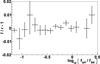 |
Fig. 7 Here we consider photometric accuracy as a function of galactic flux. No significant bias is observed. |
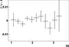 |
Fig. 8 Here we consider photometric accuracy as a function of image quality. No significant bias is observed. |
7.5.3. Photometric uncertainty results
The output covariance matrix includes the Poisson noise of the sky and the signal
itself (both star and galaxy if present). We assume that there exists an additional
quadratic term which describes contributions to the variance coming from errors in the
PSF model, the photometric ratio, and/or the residual photometric non-uniformity in the
images. The variance therefore takes the form: 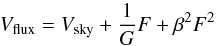 (22)where G is the gain in
e− per ADU. To estimate the value of β,
we use the photometry of bright (non variable) tertiary stars. For such stars, we assume
that the β2F2 term dominates the
variance. Fitting a linear relationship between the RMS of a high flux lightcurve and
its average flux should therefore yield the value of β. In Fig. 9, we see the result of the fit, for which we obtain
(5.6 ± 0.1) × 10-3. This is essentially identical to the repeatability of 6
mmag for aperture measurements on the same data set reported in Sect. 4.1 of Betoule et al. (2013). We are then tempted to
attribute most of this noise floor to flat fielding rather than photometry techniques.
(22)where G is the gain in
e− per ADU. To estimate the value of β,
we use the photometry of bright (non variable) tertiary stars. For such stars, we assume
that the β2F2 term dominates the
variance. Fitting a linear relationship between the RMS of a high flux lightcurve and
its average flux should therefore yield the value of β. In Fig. 9, we see the result of the fit, for which we obtain
(5.6 ± 0.1) × 10-3. This is essentially identical to the repeatability of 6
mmag for aperture measurements on the same data set reported in Sect. 4.1 of Betoule et al. (2013). We are then tempted to
attribute most of this noise floor to flat fielding rather than photometry techniques.
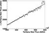 |
Fig. 9 Standard deviation of flux estimates over the lightcurve as a function of the average flux. The relation is shown here for high-flux field stars, and we see a clear linear relationship, indicative of a contribution to scatter beyond shot noise from the sky and the object. |
We check that the fitted value is accurate in the low flux regime of the fake SN. To do so, we compare the squared RMS of their light curves with the estimated variance before and after adding a quadratic correction. Note that because the galaxy flux contributes to the variance, we look at the evolution of the variance as a function of the sum of the fake star and galaxy fluxes. This is seen in Fig. 10. We see that the fitted quadratic term is compatible with data at these low fluxes, but is also almost negligible for such dim objects.
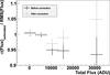 |
Fig. 10 We plot here the ratio of the modeled uncertainty to the rms of the lightcurve, as a function of the sum of the fluxes of the fake star and galaxy. The two sets of points refer to before and after adding a β term to the model uncertainty (Eq. (22)). We see that the correction makes only a small difference. |
7.5.4. Position reconstruction results
By assuming that the position fit of the model star is perfectly accurate, we can conclude that the actual position of the fake star is that of the model plus the displacement vector used during fake star construction. We are therefore able to compare the fake star’s fitted position with what we can reasonably assume is the correct one. In Fig. 11, we plot the ratio of the error on position computed in this way to the average seeing in the image sample in which the fake star was generated versus the S/N. We also plot the expected relationship between the two as explained in Appendix A.
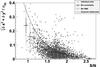 |
Fig. 11 We consider the error in the fitted position in units of σIQ as a function of the S/N. The discrepancy between the expected relationship (solid line) and observed values (points with error bars) is due to the fact that the form factor model does not accurately capture the non gaussianities of the PSF. This is explained in detail in Appendix A. The outliers observed are thought to be due to model stars affected by proper motions not detected by simultaneous astrometry. |
We notice that while the position errors follow the expected trend, a few outliers remain. We attribute these to be due to model stars affected by significant proper motions that have not been flagged as moving during simultaneous astrometry.
8. Calibration using field stars
8.1. Calibration scheme
The magnitudes delivered by the Betoule et al.
(2013) catalog, referred to as mAPER, are the result
of a comparison of tertiary star aperture fluxes with those of standard stars. Because SN
photometry is done using PSF photometry, computing a zero point requires comparing PSF and
aperture fluxes for all tertiary stars. The PSF photometry zero point for each image stack
(all images in the same field, band, and CCD) is given by:  (23)where
  is the average flux over all images in the stack. The linearity of the PSF fluxes has been
shown using the simulations discussed previously. However, the calibration of the science
images relies on the comparison of PSF and aperture fluxes. To ensure the linearity of the
entire calibration process, we must ensure the linearity of the ratio between these two.
In this section, we discuss two significant biases in the ratio of
to
is the average flux over all images in the stack. The linearity of the PSF fluxes has been
shown using the simulations discussed previously. However, the calibration of the science
images relies on the comparison of PSF and aperture fluxes. To ensure the linearity of the
entire calibration process, we must ensure the linearity of the ratio between these two.
In this section, we discuss two significant biases in the ratio of
to  ,
and what has been done to resolve them:
,
and what has been done to resolve them:
-
First, aperture photometry makes no attempt at accounting forsky subtraction residuals. In other words, the obtained flux will beartificially modified by the total flux contribution of sky residualsin the aperture. On the other hand, PSF photometry actually fitsthe remaining sky level integrated by aperture photometry (this isthe si term of Eq. (14)). Imperfections of sky subtraction lead to a bias, particularly significant at low fluxes.
-
Secondly, PSF photometry does not take into account the chromatic dependence of the PSF. The model assumes that the PSF is the same for all stars, regardless of color, which obviously leads to a color dependency in the produced PSF fluxes. Because aperture photometry does not depend much on the shape of the PSF, it is not affected by this. This also leads to a significant difference.
8.2. The effects of sky subtraction residuals
The sky level subtracted from the images is obtained using the average of the image
pixels computed over all pixels, except for masks placed over all detected objects (see
Sect. 3.1). Despite these masks, residual
contamination from the tails of the flux distribution of bright objects affect the
remainder of the image. We note that a prominent criteria in the selection of tertiary
calibration stars is their level of isolation, and they will therefore be systematically
less contaminated than the average pixels over which the sky level was computed. This is
why residual sky level at the position of tertiary calibration stars does
not average out to 0 when averaged over all images for any given star. Note that such an
effect manifests itself as a flux dependent bias because the same residual sky level will
affect the ratio of
to
more significantly for lower fluxes. This is seen clearly in Fig. 13a. It is possible to compute the expected residual effect by
comparing the PSF tail pollutions expected at the average distance from the nearest bright
objects for tertiary stars to the average PSF tails pollutions over the pixels used to
compute the sky level (see Fig. 17 of Betoule et al.
2013). Indeed, the calibration catalogs given employ such a correction.
Such a correction provides only a crudely averaged estimate of the effect. Indeed, this only produces one single correction to be applied to all stars equally. During the calibration process described here, we undo this correction (using the figures provided in Sect. 4.3.4 of Betoule et al. 2013) and implement our own. By using the fitted sky level of PSF photometry, we can instead provide one correction per star. However, such a correction only makes sense if we can reasonably believe that the fitted sky level actually corresponds to the left-over sky level. We expect for the fit to make up for errors in the PSF model by artificially altering the fitted sky level with a fraction of star’s actual flux while the actual sky level does not scale with the star flux. To allow for a chromatic component to PSF modeling errors (discussed in Sects. 8.3 and 10), we model the fitted sky level as:
![Mathematical equation: \begin{eqnarray} &&\hat{s} \,=\,[a + b \times (g - i) ] \hat{f}_{\rm PSF} + \hat{s}^{\prime}; \label{eq:sky_model}\nonumber \\ &&\hat{s}: \mbox{is the average fitted sky level}; \nonumber \\ && g ~ {\rm and} ~i: \mbox{are the g and i magnitudes respectively}; \nonumber \\ && \hat{s}^{\prime}: \mbox{is the new estimate of the average sky level}; \nonumber \\ && a ~ {\rm and} ~ b: \mbox{are fitted parameters.} \end{eqnarray}](/articles/aa/full_html/2013/09/aa21668-13/aa21668-13-eq153.png) (24)The a term is meant to
accommodate both that colors are arbitrarily defined, and that achromatic PSF errors cause
transfers between object flux and sky level. By definition, ŝ′ is
expected to be the true sky level and hence not to scale with
(24)The a term is meant to
accommodate both that colors are arbitrarily defined, and that achromatic PSF errors cause
transfers between object flux and sky level. By definition, ŝ′ is
expected to be the true sky level and hence not to scale with
 .
So, ŝ′ becomes negligible at the high-flux end of our stars, and we fit
a and b in this regime, thus rewriting definition
24 as:
.
So, ŝ′ becomes negligible at the high-flux end of our stars, and we fit
a and b in this regime, thus rewriting definition
24 as: 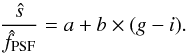 (25)The fitted relation is illustrated in Fig.
12 and the a and
b values for each band are displayed in Table 1.
(25)The fitted relation is illustrated in Fig.
12 and the a and
b values for each band are displayed in Table 1.
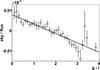 |
Fig. 12 Ratio of the fitted sky level to the flux of the star as a function of color, for high flux stars only in i band. For such stars we assume that the fitted sky level is predominantly a fraction of the flux incorrectly fitted as the sky level. We see that the fraction of flux that goes into our sky level estimator evolves linearly with color. |
Using these new ŝ′ sky values, we can correct the aperture fluxes from
Betoule et al. (2013), using their standard
aperture area: ![Mathematical equation: \begin{equation} N_{\rm APER}^{\rm effective} = \pi \left[ 7.5 \times \langle \sigma_{\rm IQ} \rangle \right ]^2 \label{eq:area_aper} \end{equation}](/articles/aa/full_html/2013/09/aa21668-13/aa21668-13-eq161.png) (26)where the effective
σIQ used is also given by the Betoule et al. (2013) downloadable catalogs.
(26)where the effective
σIQ used is also given by the Betoule et al. (2013) downloadable catalogs.
Since the sky values are fitted in units of the PSF fluxes, we instead add this
correction to PSF fluxes. These two methods are perfectly equivalent. The new zero point
averaging scheme therefore becomes:  (27)where
  is defined in Eq. (26). Using these corrections, we are able to
eliminate the magnitude bias of the zero point residuals, as shown in Fig. 13b: the zero point residuals become flat over the
entire range of used magnitudes. This is good evidence that we have, on the one hand,
properly understood the origin of this bias, and, on the other hand, properly understood
the fitted sky level.
is defined in Eq. (26). Using these corrections, we are able to
eliminate the magnitude bias of the zero point residuals, as shown in Fig. 13b: the zero point residuals become flat over the
entire range of used magnitudes. This is good evidence that we have, on the one hand,
properly understood the origin of this bias, and, on the other hand, properly understood
the fitted sky level.
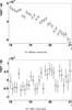 |
Fig. 13 Plot of zero point residual vs. magnitude in i band, before and after correcting for aperture sky pollutions. |
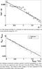 |
Fig. 14 Comparison of data with Pickles (1998) spectroscopic library in order to fit an appropriate effective filter, in g band. |
8.3. PSF chromaticity
In Fig. 14a, we display the values of the
zero-point residuals as a function of star color after application of the sky level
correction just discussed. A clear chromatic difference is observed. We interpret this
trend as resulting from the chromaticity of the PSF which is not accounted for in the PSF
model: blue and red stars are measured using the same PSF model, although blue stars are
fatter than red stars (except in z band where the effect is apparently
reversed). Such an effect is expected because IQ tends to improve towards red wavelengths.
We call α the slope of the observed relation. Its value is significant
enough that the effect must be corrected, in particular in g band. We set
out to construct a natural magnitude system for PSF fluxes that circumvents this effect.
In other words, we want to be able to convert PSF fluxes to magnitudes despite having no
knowledge of the object’s color. Explicitly, we want to be able to write:
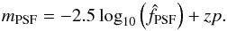 (28)It is clear from this requirement that PSF
magnitudes will differ from aperture magnitudes via a color term:
(28)It is clear from this requirement that PSF
magnitudes will differ from aperture magnitudes via a color term:  (29)where, for the time being, ϵ
is an arbitrary offset that we have not yet constrained. Note that in the AB magnitude
system, cAB is 0 by definition. We write it nonetheless to
emphasize that the relevant color term is the color difference relative to
the standard used. Recall now the definition of magnitude for a given spectral
energy density φ(λ), given in Fukugita et al. (1996). For the aperture magnitudes given in the
calibration catalog it is:
(29)where, for the time being, ϵ
is an arbitrary offset that we have not yet constrained. Note that in the AB magnitude
system, cAB is 0 by definition. We write it nonetheless to
emphasize that the relevant color term is the color difference relative to
the standard used. Recall now the definition of magnitude for a given spectral
energy density φ(λ), given in Fukugita et al. (1996). For the aperture magnitudes given in the
calibration catalog it is:  (30)The transmission function
T(λ) used is that derived in Betoule et al. (2013). We choose to construct our own natural magnitude
system for PSF fluxes using an additional effective filter
C(λ), because ignoring the PSF dependence on
wavelength favors red wavelengths over blue wavelengths (except for z
band where the effect goes the other way). In other words, for a given spectral energy
density φ(λ), the PSF magnitude is given by:
(30)The transmission function
T(λ) used is that derived in Betoule et al. (2013). We choose to construct our own natural magnitude
system for PSF fluxes using an additional effective filter
C(λ), because ignoring the PSF dependence on
wavelength favors red wavelengths over blue wavelengths (except for z
band where the effect goes the other way). In other words, for a given spectral energy
density φ(λ), the PSF magnitude is given by:
 (31)This effective filter is chosen in such a way
that it emulates the chromatic discrepancy between PSF and aperture magnitudes described
in Eq. (29). We chose to parametrize this
extra-filter as a linear function of wavelength. In effect, we require that for a given
spectroscopic library of stars (here we used the Pickles
1998 library), the difference between PSF and aperture magnitudes described in
Eqs. (30) and (31) has the same chromatic dependency as that
described in Eq. (29). In Fig. 14b, we see that the constructed linear filter can
indeed produce the required chromatic dependency. It is clear from the definitions of
mPSF and mAPER that the two
yield the same value for φAB. It is also clear from Fig. 14b that the discrepancy between the two magnitude
systems is not 0 for a typical star whose color is the same as that of AB, because of the
peculiarity of the AB spectral energy density. This constrains the free offset term
ϵ in Eq. (29) in that
it must account for this. In other words, to convert the magnitude of a star from the
aperture system to the PSF one, in addition to a color correction term
α(c − cAB), we must also
apply an offset ϵ which corresponds to the magnitude discrepancy between
the 2 systems at the color of AB. The values obtained for α and
ϵ are presented in Table 2, with
a description of the constructed linear filter used to obtain them.
(31)This effective filter is chosen in such a way
that it emulates the chromatic discrepancy between PSF and aperture magnitudes described
in Eq. (29). We chose to parametrize this
extra-filter as a linear function of wavelength. In effect, we require that for a given
spectroscopic library of stars (here we used the Pickles
1998 library), the difference between PSF and aperture magnitudes described in
Eqs. (30) and (31) has the same chromatic dependency as that
described in Eq. (29). In Fig. 14b, we see that the constructed linear filter can
indeed produce the required chromatic dependency. It is clear from the definitions of
mPSF and mAPER that the two
yield the same value for φAB. It is also clear from Fig. 14b that the discrepancy between the two magnitude
systems is not 0 for a typical star whose color is the same as that of AB, because of the
peculiarity of the AB spectral energy density. This constrains the free offset term
ϵ in Eq. (29) in that
it must account for this. In other words, to convert the magnitude of a star from the
aperture system to the PSF one, in addition to a color correction term
α(c − cAB), we must also
apply an offset ϵ which corresponds to the magnitude discrepancy between
the 2 systems at the color of AB. The values obtained for α and
ϵ are presented in Table 2, with
a description of the constructed linear filter used to obtain them.
Finally, this means that in fitting a zero point by comparing PSF fluxes to aperture
magnitudes we must take care to add a color correction term and Eq. (27) becomes:  (32)Switching spectroscopic libraries changes the
value of ϵ by about 10-4 mag or less depending on the band.
There is therefore no significant systematic error associated with this magnitude system
transformation.
(32)Switching spectroscopic libraries changes the
value of ϵ by about 10-4 mag or less depending on the band.
There is therefore no significant systematic error associated with this magnitude system
transformation.
Color terms and offsets between PSF and aperture natural magnitude systems in each band.
Finally, we consider the implications that PSF chromaticity can, in part, be due to atmospheric effects, and that the resulting color term might then vary with IQ. We have fitted the slope of Fig. 14a separately for IQs below and above the median IQ, and have found extremely compatible values. We hence conclude that a single color term can effectively describe the chromatic effects independently of IQ.
9. SN photometry
9.1. Performance on SNLS supernovae
The SNLS observing strategy calls for multiple images per night. By assuming that the
supernova flux does not evolve significantly during the night, we can fit a new lightcurve
where all fluxes in the same night have been averaged. Namely, we minimize  (33)over the vector of fluxes per night
Fn, where
Fi if the vector of measured fluxes over
individual images, Wi the inverse of their covariance matrix, and
A is a rectangular matrix filled with 1’s at positions that assign images
to nights, and 0’s elsewhere. The χ2 of such a fit yields a
good quality test of the photometry used, because it measures the compatibility of fluxes
measured over the same night. Note that this fit is weighed without taking into account
the shot noise of the SN itself. Because the shot noise is estimated using the signal
itself, such a weighing scheme would be biasing, because negative fluctuations would
receive larger weights than positive ones (see e.g. Humphrey et al. 2009, and references therein).
(33)over the vector of fluxes per night
Fn, where
Fi if the vector of measured fluxes over
individual images, Wi the inverse of their covariance matrix, and
A is a rectangular matrix filled with 1’s at positions that assign images
to nights, and 0’s elsewhere. The χ2 of such a fit yields a
good quality test of the photometry used, because it measures the compatibility of fluxes
measured over the same night. Note that this fit is weighed without taking into account
the shot noise of the SN itself. Because the shot noise is estimated using the signal
itself, such a weighing scheme would be biasing, because negative fluctuations would
receive larger weights than positive ones (see e.g. Humphrey et al. 2009, and references therein).
In Fig. 15 we provide the χ2/Nd.o.f. distribution of these fits and the average value is very close to 1. This is particularly true for high redshift SN, where uncertainty terms scaling with flux are negligible. Indeed, we see in Fig. 16 a clear increase of the χ2/Nd.o.f. for low redshift SN, where this noise is no longer completely negligible. Note that the dispersion is as expected for a χ2 distribution, given the number of degrees of freedom for each fit.
9.2. Band-to-band position transformations
A significant difference between SN and tertiary star photometry comes from the fact that the SN position is not fitted in g and z bands due to the expected low S/N. Instead, we transfer the fitted position from the r and/or i bands. To transfer the SN position from, for example, r to g, we evaluate the position of stars in both astrometric catalogs at the epoch of the reference image in g band using the fitted proper motions, fit the geometric transformation that maps r positions to the ones in g, and apply this transformation to the SN position in r band. We then fit the SN in g at this fixed position.
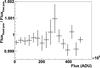 |
Fig. 17 Ratio of the fitted flux at fixed position to the fitted flux with free position as a function of flux. We see no clear flux dependence in the flux underestimation resulting from the transformation. |
To ensure that this does not lead to significant differences between SN and tertiary star photometry, we do the same for a sizable number of tertiary stars (more precisely: all tertiary stars in g band in the D1 field). In other words, we compute lightcurves for these stars at fixed positions using their fitted position in r band, after transferring it in the same way we do for SNe. We then compare the lightcurves obtained with those fitted in the regular way, i.e. fitting both fluxes and position. In Fig. 17, we find that the transformation incurs a flux underestimation of about 4 × 10⁻⁴ independently of the flux of the object considered. In comparing the difference between the fitted position in g band and the transferred position from r band, it is clear that the difference is dominated by the y coordinate term. In Fig. 18, we see a clear trend between the discrepancy in y and the color of the star, pointing to a refraction effect.
Note that, as discussed previously (Sect. 6.2), when fitting astrometry within an image series (i.e. images in the same band) we are sensitive to the scatter of the refraction displacements about the average position. Here, however, we are transferring a position from one band to another, and we are therefore concerned with the difference in the average displacement between the 2 bands. Because for the SNLS we have that E [tanzcosη] is much greater than E [tanzsinη], we can understand why, recalling Eqs. (9) and (10), the effect is much greater along y than along x. In Table 3, we provide the expectation values and RMS of tanzcosη and tanzsinη across all fields and filters. We find that we do not expect the effect to be much more significant in other fields, and other bands are less affected. Using the Pickles (1998) library, and computing the atmopheric refraction shifts for a standard Mauna Kea air column at tanzsinη = 0.48, we are able to reproduce the slope displayed in Fig. 18.
The effect is most important when transporting coordinates into g band, because the variation of the refractive index of air decreases with wavelength. In order to assess the effect on supernovae, we propagate the average g − i color of supernovae as a function of redshift z (g − i ≃ 3.6 × z − 0.75) through the relation displayed in Fig. 18, and input the found displacement into expression (3). We find a relative flux bias that varies from 0.5 × 10⁻³ at z = 0.2 (lowest SNLS redshifts) to ~0 at z = 0.6 (beyond which g is no longer used to estimate distances). This refraction-induced bias is hence negligible.
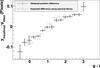 |
Fig. 18 Difference between the fitted position in g band and the transformed position from r band as a function of color. This is done for all stars in the D1 field. We also plot the expected difference obtained by computing the atmopheric refraction shifts for the stars in Pickles (1998). |
Average and standard deviation of tanzcosη and tanzsinη for each field, across all bands.
10. Does the PSF size evolve with brightness?
The photometry methods we have been discussing so far assume that the PSF shape does not vary with flux at fixed color. If it does, the flux ratios of supernovae to field stars become biased. We now study how firmly this hypothesis is confirmed by measurements.
In Fig. 19, we show that the apparent size of stars, defined from their Gaussian-weighted second moments (implicitly defined by Eq. (1)) tends to grow linearly with the peak flux (fmax) of this star. This “brighter-fatter” relation is however shallow: sizes change by about 0.008 pixel over the whole brightness range, i.e. less than 0.5% for this sample.
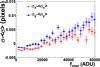 |
Fig. 19 Difference of second moments of stars to the average (over 1 CCD), as a function of peak flux. This is measured on a small set of r-band frames taken at low Galactic latitude, which have < σIQ > ≃ 1.8 pixel. From vanishing to almost saturating stars, the apparent size of stars seem to vary essentially linearly with peak flux by about 0.5%. |
To first order, the relative flux biases from PSF photometry are exactly the ratio of the assumed PSF size to the true size. One can check that statement for both Gaussians and Moffat PSFs. In what follows, we discuss the relative size change σ/ ⟨σ⟩ − 1 of a given star with respect to a local average ⟨σ⟩, because this describes the expected size of PSF flux biases from a wrong assumed PSF size.
We know that, due at least to atmospheric effects and electron diffusion in the sensors, the “size” of stars (in a given band) depends on their color. Since in a given sample of measurements, flux and colors are usually related, we first measure this color vs. size dependence by restricting the analysis to the low-flux regime. We then measure the actual rise of apparent size with peak flux after accounting for the size-color relation. Both relations are illustrated in Fig. 20 for the g band and y direction, and the fitted slopes in all bands for both correlations and both coordinates are provided in Table 4. We note that the size-color relations are broadly compatible with the color terms of PSF vs. aperture magnitudes of Table 2. We also note that we do observe a color-independent brighter-fatter relations, which are slightly but consistently steeper along y than along x and similar across bands. Accounting for the size-color relation is mandatory in g and r bands, but does not significantly change the results in redder bands. Note that requiring that e.g. g − i is measured introduces a relation between fmax in g band and color because bright stars in g tend to saturate in i band if they are red.
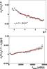 |
Fig. 20 Relative difference of second moments of stars to the average (over 1 CCD), as a function of g − i color (top), for faint stars, and as a function of peak flux (bottom), correcting for the size-color relation Both plots display the science data, in g band. Values for the slopes in all bands are provided in Table 4. |
Slopes of size vs. color and size vs. fmax relations.
Because calibration stars are significantly brighter than supernovae, their PSF flux ratio measured using the same PSF are biased due to this PSF size change. However, the calibration stars have a peak flux at most of 20 000 ADU, and on average of about 5000 ADU. So, given the slopes in Table 4, the relative flux biases between supernovae and tertiaries are around 3 × 10⁻⁴, and can hence be ignored.
Instead of these a posteriori arguments, it would be more appropriate to incorporate the change of PSF size with flux into the PSF model. It would have been our policy had we realized early enough the existence of the effect. Indeed, we discovered its existence while analyzing test bench data from other sensors6. In both instances, we find that the size rise is faster by about 20% along y (CCD columns) than along x (CCD rows). We do not find evidence of a significant variation from band to band. Because the brighter-fatter effect seems linear with flux on two different sensors, it is tempting to attribute it to a physical effect within the sensor, rather than some non-linearity of the electronic chain. One possible cause might be that charges stored in the CCD induced by bright objects repel forthcoming charges, thus causing the broadening.
11. Practical implementation of the simultaneous photometry algorithms
The cores of both codes, written in C++, are Newton-Raphson minimizers which require computation of both the gradient and the Hessian of the χ2. We use analytical derivatives for all parameters, and the Hessian computation dominates the CPU budget. The algorithms require an input position for the source (or the source list), and the first minimization step is carried out at the fixed input position in order to derive fluxes, which are required to evaluate the derivatives with respect to position. Then, the position is released and the required fit is carried out, which typically converges in 5 iterations. Because it fits larger stamps, the RSP algorithm is 2 to 3 times slower than the DSP algorithm. The latter fits a supernova lightcurve with its underlying galaxy on ~700 images in about 2500 s on typical ~2 GHz recent computers. On the same image set, fitting lightcurves of ~100 tertiaries (without an underlying galaxy) takes about 2 h. Neither of the codes has been aggressively optimized.
12. Summary and conclusions
We have presented two photometric methods to measure lightcurve of supernovae in the framework of the SNLS. Both methods have been tested using realistic simulations which consist in adding artificial supernovae to real images by copying artificially dimmed real stars, and comparing the measured and the applied dimming. The RSP method exhibits a marginally significant bias of ~2 ± 1 mmag, which survived numerous tests, and that we hence attribute to statistical fluctuation (Sect. 7.5.1). The non-resampling method DSP appears free of biases to a similar 1 mmag accuracy (Sect. 7.5.2). We have also derived an uncertainty model that accurately describes the scatter observed in simulations by adding a systematic noise floor of 6 × 10⁻³ to propagated shot noise contributions (Sect. 7.5.3). In practise, the DSP method is faster (mostly because it does not require resampling) and more firmly founded from a statistical point of view (because it does not ignore pixel correlations introduced by resampling) and should hence be prefered over the RSP method. The DSP method also allows one to over-sample the galaxy model while the RSP method does not.
We have established the methods required to accurately compare aperture calibrated magnitudes with instrumental PSF magnitudes of the field stars, required to attribute calibrated magnitudes to supernovae. Two effects have to be corrected for:
-
systematic biases of PSF fluxes due to the wavelength dependence of the PSF, ignored in the PSF model. This translates into effective PSF bandpasses slightly different from aperture bandpasses. We model the difference between these two sets of bandpasses using the color terms between both sets of magnitudes (Sect. 8.3);
-
systematic biases of the estimated sky level in aperture photometry due to the tertiary stars being more isolated than average, and hence being less contaminated by light from other objects in the field than average objects. We correct for this effect using the sky level measured from the simultaneous PSF photometry (Sect. 8.2). We first have to correct for colored systematic contributions to this estimated sky level, due to the wavelength dependence of PSF mentionned just above.
From Figs. 13 and 14, we generously attribute an uncertainty of these two operations of 1 mmag. Together with the uncertainty of 1 mmag for the SN to tertiaries flux ratio, magnitudes of supernovae are affected by an uncertainty of ~1.5 mmag with respect to calibrated aperture magnitudes of tertiary stars. This is significantly smaller than the systematic uncertainties affecting the physical fluxes of these tertiary stars, which are on the order of ~4−5 mmag (Table 23 of Betoule et al. 2013).
Our photometric method requires a determination of the relative astrometry of individual images involved in the measurements and we reach a positional floor uncertainty of 2.4 mas per star, image and coordinate, independent of the band (Sect. 6.1). This precision allows us to detect tiny variations of CCD row physical size (Appendix B). We investigate effects of refraction on relative astrometry within a band (Sect. 6.2) and across bands (Sect. 9.2) and conclude that it can be ignored in both cases. We eventually detect that bright stars tend to appear slightly “fatter” than faint stars, but this effect does not significantly affect our photometry and calibration procedure.
In statistics, the efficiency of an estimator is defined as the ratio of the minimum variance bound (from the Cramér-Rao inequality) to its actual variance (see e.g. Kendall & Stuart 1961, Sect. 18.15).
The model of Eq. (6) is unchanged if one
operates the simultaneous substitutions:
galref ← galref + C
and  .
.
The Gauss-Markov theorem states that for Gaussian problems, among linear estimators, the one with smallest variance maximises the likelihood.
For sake of completeness, we note that rather than fitting T, we fit the reciprocal functions because the fit is then linear.
We are grateful to Doherty (Harvard University) for providing us with test data of a candidate sensor for LSST.
Acknowledgments
J. Marriner kindly accepted to read the manuscript, and we gratefully followed most of his suggestions. This paper relies on a very large set of high-quality images acquired by Queue Service Observing team at CFHT. This research used the facilities of the Canadian Astronomy Data Centre operated by the National Research Council of Canada with the support of the Canadian Space Agency. The authors heavily rely on the Centre de calcul de l’IN2P3 for computing and data storage.
References
- Alard, C. 2000, A&AS, 144, 363 [NASA ADS] [CrossRef] [EDP Sciences] [Google Scholar]
- Alard, C., & Lupton, R. H. 1998, ApJ, 503, 325 [NASA ADS] [CrossRef] [Google Scholar]
- Anderson, J., & King, I. R. 1999, PASP, 111, 1095 [NASA ADS] [CrossRef] [Google Scholar]
- Anderson, J., Bedin, L. R., Piotto, G., Yadav, R. S., & Bellini, A. 2006, A&A, 454, 1029 [NASA ADS] [CrossRef] [EDP Sciences] [Google Scholar]
- Astier, P., Guy, J., Regnault, N., et al. 2006, A&A, 447, 31 [NASA ADS] [CrossRef] [EDP Sciences] [Google Scholar]
- Barris, B. J., Tonry, J. L., Novicki, M. C., & Wood-Vasey, W. M. 2005, AJ, 130, 2272 [NASA ADS] [CrossRef] [Google Scholar]
- Bertin, E., & Arnouts, S. 1996, A&AS, 117, 393 [NASA ADS] [CrossRef] [EDP Sciences] [Google Scholar]
- Betoule, M., Marriner, J., Regnault, N., et al. 2013, A&A, 552, A124 [NASA ADS] [CrossRef] [EDP Sciences] [Google Scholar]
- Boulade, O., Charlot, X., Abbon, P., et al. 2003, in Instrument Design and Performance for Optical/Infrared Ground-based Telescopes, eds. I. Masanori, & A. F. M. Moorwood, Proc. SPIE, 4841, 72 [Google Scholar]
- Conley, A., Guy, J., Sullivan, M., et al. 2011, ApJS, 192, 1 [NASA ADS] [CrossRef] [EDP Sciences] [Google Scholar]
- Fabbro, S. 2001, Ph.D. Thesis, Université Denis Diderot, Paris [Google Scholar]
- Fukugita, M., Ichikawa, T., Gunn, J. E., et al. 1996, AJ, 111, 1748 [NASA ADS] [CrossRef] [Google Scholar]
- Guy, J., Sullivan, M., Conley, A., et al. 2010, A&A, 523, A7 [NASA ADS] [CrossRef] [EDP Sciences] [Google Scholar]
- Hamuy, M., Phillips, M. M., Maza, J., et al. 1994, AJ, 108, 2226 [NASA ADS] [CrossRef] [Google Scholar]
- Holtzman, J. A., Marriner, J., Kessler, R., et al. 2008, AJ, 136, 2306 [NASA ADS] [CrossRef] [Google Scholar]
- Humphrey, P. J., Liu, W., & Buote, D. A. 2009, ApJ, 693, 822 [NASA ADS] [CrossRef] [Google Scholar]
- Irwin, M. J. 1985, MNRAS, 214, 575 [NASA ADS] [Google Scholar]
- Ivezić, Ž., Smith, J. A., Miknaitis, G., et al. 2007, AJ, 134, 973 [NASA ADS] [CrossRef] [Google Scholar]
- Jenkins, J. M., Caldwell, D. A., Chandrasekaran, H., et al. 2010, ApJ, 713, L120 [NASA ADS] [CrossRef] [Google Scholar]
- Kendall, M. G., & Stuart, A. 1961, The advanced theory of statistics: Inference and relationship (Charles Griffin), Vol. 2 [Google Scholar]
- Landolt, A. U. 1992, AJ, 104, 340 [NASA ADS] [CrossRef] [Google Scholar]
- Lazorenko, P. F. 2006, A&A, 449, 1271 [NASA ADS] [CrossRef] [EDP Sciences] [Google Scholar]
- Magnier, E. A., & Cuillandre, J.-C. 2004, PASP, 116, 449 [NASA ADS] [CrossRef] [Google Scholar]
- Moffat, A. F. J. 1969, A&A, 3, 455 [NASA ADS] [Google Scholar]
- Montalto, M., Piotto, G., Desidera, S., et al. 2007, A&A, 470, 1137 [NASA ADS] [CrossRef] [EDP Sciences] [Google Scholar]
- Perlmutter, S., Aldering, G., Goldhaber, G., et al. 1999, ApJ, 517, 565 [NASA ADS] [CrossRef] [Google Scholar]
- Pickles, A. J. 1998, PASP, 110, 863 [CrossRef] [Google Scholar]
- Schmidt, B. P., Suntzeff, N. B., Phillips, M. M., et al. 1998, ApJ, 507, 46 [NASA ADS] [CrossRef] [Google Scholar]
- Smith, J. A., Tucker, D. L., Kent, S., et al. 2002, AJ, 123, 2121 [Google Scholar]
- Stetson, P. B. 1987, PASP, 99, 191 [NASA ADS] [CrossRef] [Google Scholar]
- Sullivan, M., Guy, J., Conley, A., et al. 2011, ApJ, 737, 102 [NASA ADS] [CrossRef] [Google Scholar]
- Tucker, D. L., Kent, S., Richmond, M. W., et al. 2006, Astron. Nachr., 327, 821 [NASA ADS] [CrossRef] [Google Scholar]
Appendix A: Form factor for displacement errors
To get to Eq. (3) we rely on the key
assumption that the PSF is nearly identical to a Gaussian for which
σx = σy = σseeing & σxy = 0.
To account for errors induced by this assumption, we allow for an additional form factor
F in Eq. (3) which then
takes the form: ![Mathematical equation: \appendix \setcounter{section}{1} \begin{equation} {E}[\hat{f}] = f \left\{ 1 - F \times \frac{(\Delta x)^2 + (\Delta y)^2}{4 \sigma ^2} \right\} \label{eq:formfactor} \end{equation}](/articles/aa/full_html/2013/09/aa21668-13/aa21668-13-eq207.png) (A.1)To find the value of F, we
use the exact expression for the flux estimator expectation for any given PSF model which
is:
(A.1)To find the value of F, we
use the exact expression for the flux estimator expectation for any given PSF model which
is: ![Mathematical equation: \appendix \setcounter{section}{1} \begin{equation} {E}[\hat{f}] = f \frac{{E}[\int \overbrace{{\rm PSF}(x,y)}^{\rm Data} \overbrace{{\rm PSF}(x-\hat{\delta _x},y-\hat{\delta _y}}^{\rm Fitted\,\, PSF}) {\rm d}x {\rm d}y]}{\int {\rm PSF}^2(x,y) {\rm d}x {\rm d}y} \label{eq:PSFerr} \end{equation}](/articles/aa/full_html/2013/09/aa21668-13/aa21668-13-eq208.png) (A.2)We then compute Eq. (A.2) numerically for a range of displacements
using the PSF model of the reference image. When fitting Eq. (A.1) to the results we obtain
F = 0.788.
(A.2)We then compute Eq. (A.2) numerically for a range of displacements
using the PSF model of the reference image. When fitting Eq. (A.1) to the results we obtain
F = 0.788.
Appendix B: Pixel size variations
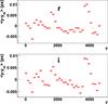 |
Fig. B.1 Average astrometric residuals along y (expressed in pixels) as a function of the y coordinate of measurements, for measurements in CCD 12 of stars brighter than 20.5. The average runs over the 4 SNLS science fields, i.e. ~2000 r images and ~3000 i images. The shape is very similar in r- and i-bands, suggesting some instrumental source. The jumps of residuals happen at y values close to multiples of 512. |
 |
Fig. B.2 Stamp of a flat-field image around y = 515. The response variation around one or two rows is clearly visible, corresponding to the discontinuity of Fig. B.1. |
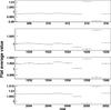 |
Fig. B.3 Flat-field average value along rows as a function of y, zoomed around some of the discontinuities of Fig. B.1. The response variation extends over a few rows and is typically on the order of 1%. They are located at y ≃ 3 + n × 512. |
The astrometric fit we have described in Sect. 6.1 assumes that positions measured in pixel units describe the physical position in the CCD, perhaps up to some very smooth variation. This is not necessarily realized: the physical pixel size might vary too rapidly for the coordinate mappings to accommodate the variation. The manufacturing of CCDs can make some rows or columns wider or narrower than the average. Figure B.1 presents the average astrometric residual along y as a function of the y position of the measurement. It exhibits discontinuities of the order of 0.01 pixel, observed at the same locations in both r and i bands, and at y values roughly multiples of 512. Figure B.2 displays a stamp of a flatfield image (r-band) where the variation of flat-field response along one or two rows is clearly visible. The flat-field average value over rows is displayed in Fig. B.3, where one can spot variations on the order of 1% of the average flat values at the positions where we detect astrometric residual discontinuities. It is tempting to attribute the latter to physically wider or narrower rows, due to some tiny misplacement of the masks during the CCD manufacturing (type E2V CCD42-90). As we do not detect any comparable pattern along x, and since the residuals along x are not smaller than along y, we cannot attribute a sizable fraction of the astrometric noise floor to these small defects. We thus did not attempt do incorporate those into the astrometric model. Similar mechanical defects with the same consequences on astrometry were discussed about the WFPC2 camera on the Hubble Space Telescope in Anderson & King (1999).
All Tables
Color terms and offsets between PSF and aperture natural magnitude systems in each band.
Average and standard deviation of tanzcosη and tanzsinη for each field, across all bands.
All Figures
|
Fig. 1 Gaussian-weighted second moments from a single typical image, with the found star clump and the star selection (red points within the ellipse). |
| In the text | |
|
Fig. 2 Astrometric 1D residuals scatter as a function of star magnitude for the D3 field in r band. The top plot compares, as a function of magnitude, the measured residual rms (points) with the average expected rms (curve) including a noise floor of 0.013 pixels. They are roughly compatible, but not necessarily equal because the expected rms varies with IQ at fixed magnitude. The bottom plot displays the rms of the residual pulls (i.e. residuals in unit of expected rms), which are close to 1 at all magnitudes. We hence conclude that adding the position noise floor of 0.013 pixels (2.4 mas) in quadrature to the position uncertainty expected from shot noise fairly describes the residuals. This figure only considers residuals along y for reasons explained in Sect. 6.2. |
| In the text | |
|
Fig. 3 Astrometric residuals along x (i.e. RA) in g band as a function of the displacement expected from refraction, up to an unknown constant, for stars brighter than i = 20. |
| In the text | |
|
Fig. 4 Above are density plots comparing the distribution of real SN and simulated fake stars in the plane of galactic flux vs. S/N. |
| In the text | |
|
Fig. 5 Photometric factor accuracy as a function of S/N for the RSP method. |
| In the text | |
|
Fig. 6 Photometric factor accuracy as a function of S/N for the DSP method. |
| In the text | |
|
Fig. 7 Here we consider photometric accuracy as a function of galactic flux. No significant bias is observed. |
| In the text | |
|
Fig. 8 Here we consider photometric accuracy as a function of image quality. No significant bias is observed. |
| In the text | |
|
Fig. 9 Standard deviation of flux estimates over the lightcurve as a function of the average flux. The relation is shown here for high-flux field stars, and we see a clear linear relationship, indicative of a contribution to scatter beyond shot noise from the sky and the object. |
| In the text | |
|
Fig. 10 We plot here the ratio of the modeled uncertainty to the rms of the lightcurve, as a function of the sum of the fluxes of the fake star and galaxy. The two sets of points refer to before and after adding a β term to the model uncertainty (Eq. (22)). We see that the correction makes only a small difference. |
| In the text | |
|
Fig. 11 We consider the error in the fitted position in units of σIQ as a function of the S/N. The discrepancy between the expected relationship (solid line) and observed values (points with error bars) is due to the fact that the form factor model does not accurately capture the non gaussianities of the PSF. This is explained in detail in Appendix A. The outliers observed are thought to be due to model stars affected by proper motions not detected by simultaneous astrometry. |
| In the text | |
|
Fig. 12 Ratio of the fitted sky level to the flux of the star as a function of color, for high flux stars only in i band. For such stars we assume that the fitted sky level is predominantly a fraction of the flux incorrectly fitted as the sky level. We see that the fraction of flux that goes into our sky level estimator evolves linearly with color. |
| In the text | |
|
Fig. 13 Plot of zero point residual vs. magnitude in i band, before and after correcting for aperture sky pollutions. |
| In the text | |
|
Fig. 14 Comparison of data with Pickles (1998) spectroscopic library in order to fit an appropriate effective filter, in g band. |
| In the text | |
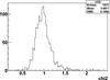 |
Fig. 15 Distribution of the χ2/Nd.o.f. of night fits (Eq. (33)) of real SNe. |
| In the text | |
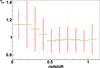 |
Fig. 16 Evolution of χ2/Nd.o.f. of night fits (Eq. (33)) of real SNe with their redshift. |
| In the text | |
|
Fig. 17 Ratio of the fitted flux at fixed position to the fitted flux with free position as a function of flux. We see no clear flux dependence in the flux underestimation resulting from the transformation. |
| In the text | |
|
Fig. 18 Difference between the fitted position in g band and the transformed position from r band as a function of color. This is done for all stars in the D1 field. We also plot the expected difference obtained by computing the atmopheric refraction shifts for the stars in Pickles (1998). |
| In the text | |
|
Fig. 19 Difference of second moments of stars to the average (over 1 CCD), as a function of peak flux. This is measured on a small set of r-band frames taken at low Galactic latitude, which have < σIQ > ≃ 1.8 pixel. From vanishing to almost saturating stars, the apparent size of stars seem to vary essentially linearly with peak flux by about 0.5%. |
| In the text | |
|
Fig. 20 Relative difference of second moments of stars to the average (over 1 CCD), as a function of g − i color (top), for faint stars, and as a function of peak flux (bottom), correcting for the size-color relation Both plots display the science data, in g band. Values for the slopes in all bands are provided in Table 4. |
| In the text | |
|
Fig. B.1 Average astrometric residuals along y (expressed in pixels) as a function of the y coordinate of measurements, for measurements in CCD 12 of stars brighter than 20.5. The average runs over the 4 SNLS science fields, i.e. ~2000 r images and ~3000 i images. The shape is very similar in r- and i-bands, suggesting some instrumental source. The jumps of residuals happen at y values close to multiples of 512. |
| In the text | |
|
Fig. B.2 Stamp of a flat-field image around y = 515. The response variation around one or two rows is clearly visible, corresponding to the discontinuity of Fig. B.1. |
| In the text | |
|
Fig. B.3 Flat-field average value along rows as a function of y, zoomed around some of the discontinuities of Fig. B.1. The response variation extends over a few rows and is typically on the order of 1%. They are located at y ≃ 3 + n × 512. |
| In the text | |
Current usage metrics show cumulative count of Article Views (full-text article views including HTML views, PDF and ePub downloads, according to the available data) and Abstracts Views on Vision4Press platform.
Data correspond to usage on the plateform after 2015. The current usage metrics is available 48-96 hours after online publication and is updated daily on week days.
Initial download of the metrics may take a while.