| Issue |
A&A
Volume 557, September 2013
|
|
|---|---|---|
| Article Number | A68 | |
| Number of page(s) | 10 | |
| Section | Interstellar and circumstellar matter | |
| DOI | https://doi.org/10.1051/0004-6361/201220930 | |
| Published online | 02 September 2013 | |
Planet or brown dwarf? Inferring the companion mass in HD 100546 from the wall shape using mid-infrared interferometry
1
Astronomical Institute “Anton Pannekoek”, University of
Amsterdam,
PO Box 94249,
1090 GE
Amsterdam,
The Netherlands
e-mail:
This email address is being protected from spambots. You need JavaScript enabled to view it.
2
SRON Netherlands Institute for Space Research,
PO Box 800, 9700 AV
Groningen, The
Netherlands
3
DAMTP, University of Cambridge, Wilberforce Road, Cambridge
CB3 0WA,
UK
4
Institute of Astronomy, University of Cambridge,
Madingley Road, Cambridge
CB3 0HA,
UK
5
Department of Astrophysics/IMAPP, Radboud University
Nijmegen, PO Box
9010, 6500 GL
Nijmegen, The
Netherlands
6
Max-Planck Institute for Astronomy, Königstuhl 17, 69117
Heidelberg,
Germany
7
Universitäts-Sternwarte München,
Ludwig-Maximilians-Universität, Scheinerstr. 1, 81679
München,
Germany
Received: 15 December 2012
Accepted: 20 June 2013
Abstract
Context. Giant planets form in protoplanetary disks while these disks are still gas-rich, and can reveal their presence through the annular gaps they carve out. HD 100546 is a gas-rich disk with a wide gap between a radius of ~1 and 13 AU, possibly cleared out by a planetary companion or planetary system.
Aims. We aim to identify the nature of the unseen companion near the far end of the disk gap.
Methods. We used mid-infrared interferometry at multiple baselines to constrain the curvature of the disk wall at the far end of the gap. We used 2D hydrodynamical simulations of embedded planets and brown dwarfs to estimate the viscosity of the disk and the mass of a companion close to the disk wall.
Results. We find that the disk wall at the far end of the gap is not vertical, but rounded-off by a gradient in the surface density. This gradient can be reproduced in hydrodynamical simulations with a single, heavy companion (≳30...80 MJup) while the disk has a viscosity of at least α ≳ 5 × 10⁻³. Taking into account the changes in the temperature structure after gap opening reduces the lower limit on the planet mass and disk viscosity to 20 MJup and α = 2 × 10⁻³.
Conclusions. The object in the disk gap of HD 100546 that shapes the disk wall is most likely a 60+20-40 MJup brown dwarf, while the disk viscosity is estimated to be at least α = 2 × 10⁻³. The disk viscosity is an important factor in estimating planetary masses from disk morphologies: more viscous disks need heavier planets to open an equally deep gap.
Key words: radiative transfer / hydrodynamics / planet-disk interactions / stars: individual: HD 100546 / protoplanetary disks / turbulence
© ESO, 2013
1. Introduction
Giant planets need to form before the gas in protoplanetary disks is dispersed, which makes some of these disks not only planet-forming, but most likely also planet-hosting. Current planet-finding techniques have difficulties in detecting planets around these young stars: transits are blocked from view by the disk, while radial velocity measurements are disturbed by the variability of the stellar photosphere (Setiawan et al. 2008; Huelamo et al. 2008), though (interferometric) imaging has identified a few possible companions (Kraus & Ireland 2012; Quanz et al. 2013).
However, planets can also reveal themselves in an indirect way, through their dynamical impact on the protoplanetary disk (e.g. Lin & Papaloizou 1979, 1986). A gap carved by a single planet has very little impact on the spectral energy distribution (SED), but could be identified by imaging of the disk (Steinacker & Henning 2003; Varnière et al. 2006; Wolf et al. 2007). Nonetheless, a class of so-called transitional disks have been identified on the basis of their low near-infrared excess, which is apparently caused by depleted inner regions (Strom et al. 1989; Muzerolle et al. 2004; Calvet et al. 2005). Long-wavelength imaging has confirmed that most of these indeed have enlarged inner holes or annular gaps (Brown et al. 2009; Andrews et al. 2011) and their size suggests that multiple planets must be responsible (Dodson-Robinson & Salyk 2011; Zhu et al. 2011) or an additional clearing mechanism is at work, such as dust filtration or grain growth (Zhu et al. 2012; Birnstiel et al. 2012). However, how these transitional disks sustain a substantial accretion rate with a depleted inner region remains a mystery, as does the underlying architecture of their planetary systems.
If present, the properties of an underlying planetary system may be inferred from the disk geometry. Giant planets will carve out deep and wide gaps in the gas and dust, and a whole suite of codes exists to study disk-planet interactions (see de Val-Borro et al. 2006, for a comparison of these codes). Comparing these results to observational constraints on the surface density profile allows one to estimate the mass and location of a planet (e.g. Tatulli et al. 2011).
In this work, we study the disk-planet interaction in the disk of HD 100546. It was identified by Bouwman et al. (2003) as a transitional disk on the basis of its SED even before the term existed, with an estimated companion mass of ~10 MJup. The gap was later confirmed using mid-infrared nulling interferometry (Liu et al. 2003), UV spectroscopy (Grady et al. 2005), near-infrared CO spectroscopy (Brittain et al. 2009; Van Der Plas et al. 2009), and mid-infrared interferometry (Panić et al. 2012), all1 consistent with a gap outer radius in the range of 10 to 15 AU. The inner disk is depleted in dust by a few orders of magnitude (Benisty et al. 2010; Mulders et al. 2011), and is smaller than 0.7 AU in size (Panić et al. 2012). Hydrodynamical modeling of the surface density profile inferred from the SED by Tatulli et al. (2011) yields a planet of at least one Jupiter mass at 8 AU. Evidence for the presence of a more massive companion of 20 Jupiter mass within the gap has been found by Acke & van den Ancker (2006). Recent interferometric imaging has also revealed a (different) planetary candidate farther out in the disk, at 70 AU (Quanz et al. 2013).
The surface density profile around the gap can also be studied using mid-infrared interferometric data, providing additional constraints on the nature of a (planetary) companion. Using inclined ring models, Panić et al. (2012) have shown that the mid-infrared visibilities can not be reproduced by a sudden jump in intensity at the location of the disk wall at 13 AU, but that the emission from the edge increases smoothly over a few AU. This may indicate that the surface density does not show a sharp increase at 13 AU that points to a vertical wall, but gradually increases with radius. In this case the optical depth – which determines the height of the disk surface – also increases smoothly with radius, producing a more rounded-off wall. In this paper, we explore the observational appearance of these surface density profiles and how they can be explained by the gravitational and hydrodynamic interaction between a disk and a planet.
These rounded-off walls are a natural outcome of hydrodynamical models of disk-planet interaction, where the detailed shape of the radial surface density profile depends on planet mass, disk thickness, and viscosity (Crida et al. 2006; Lubow & D’Angelo 2006). The mass of the planet will therefore be reflected in the shape of the disk wall, which can be constrained with MIDI, the mid-infrared interferometer on the Very Large Telescope. We explain this in more detail in Sect. 2. In addition to the planets mass, the viscosity in the disk wall is a critical parameter in determining the gap shape.
We used a 2D radiative transfer code to model both SED and mid-infrared visibilities to determine the shape of the surface density profile in the disk wall at the far end of the gap (Sect. 3). We then tried to reproduce this surface density profile with a hydrodynamical code to constrain the planet mass and disk viscosity (Sect. 4). We discuss the companion mass and robustness of our result in Sect. 5 and summarize our results in the conclusion.
2. Interferometric signature of a disk wall
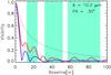 |
Fig. 1 Visibilities versus baseline length for HD 100546 at 10 micron, along a position angle of 30 degree (the same as the 41 meter baselines). The colored lines show a very round wall in blue, a steeper wall in dotted red, a vertical wall in solid red, and a model without a gap in dotted gray. Note that in the model without a gap the emission is coming from much closer to the star, and visibilities are much higher. Indicated in green are the spatial frequency ranges probed by the MIDI spectra used in this paper (λ = 8....13 micron), displayed as effective baseline at ten micron (Baseline/λ × 10 μm). |
The visibility versus baseline curve is a Fourier transform of the surface brightness profile. Therefore, the visibility curve of a continuous disk2 decreases monotonously with baseline (gray dotted line in Fig. 1), as contributions from different radii add up to a smooth curve. In this case, the visibility is a direct measure of the spatial extent of a source.
However, in a disk with a gap, the situation is much more complex. The material at the far end of the gap (disk wall) intercepts a much larger fraction of the stellar light than in a continuous disk, creating a peak in the surface brightness at that location, (red line in Figs. 2 and 3). The flux contribution from this radius will then dominate over that of the other radii, both in the SED and visibilities. Its Bessel function will contribute more to the visibilities than those from other radii, resulting in the characteristic gap signature in the visibility curve, showing multiple minima (bounces or nulls) and maxima (sidelobes) (Fig. 1, red line).
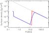 |
Fig. 2 Surface density profile of the disk for the same models as in Fig. 1. The surface density normalizations are those of the best-fit model described in Table 1. |
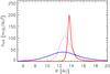 |
Fig. 3 Radial brightness profile of the disk at 12.5 μm for the same models as in Fig. 1. The model without a gap has no brightness peak in this range and is not shown. |
The detailed shape of the visibility curve of a gapped disk depends on the structure of the disk wall: a vertical wall (defined as a step function in the surface density) will create a narrow peak in the surface brightness profile with a typical width of a few AU. This non-zero width is due to inclination and optical depth effects caused by the vertical structure. It has much more power in the sidelobes, making the gap structure visible at very long baselines (red lines in Figs. 1−3). If the surface density increases gradually over a few AU (Fig. 2, blue line), the optical depth will increase more slowly, giving a surface height in the disk wall that slowly increases with radius, rounding off the wall. This round wall will create a broader peak in the surface brightness profile (Fig. 3, blue line). As shown in Panić et al. (2012), this puts less power in the sidelobes, because overlapping Bessel functions cancel each other out, resulting in a smoother curve where the gap signature is not visible at longer baselines (Fig. 1, blue line).
The shape of the disk wall at the far end of the gap can therefore be directly derived from the amount of structure in the visibility curve at long baselines. This method has been applied in the near-infrared to study the shape of inner rims at the dust sublimation radius (e.g. Tannirkulam et al. 2008; Dullemond & Monnier 2010,their Fig. 5). Indications for a round wall are also found with mid-infrared interferometry in the disk of TW Hya (Ratzka et al. 2007).
We used this method to derive the shape of the surface density profile in the disk wall from the MIDI observations presented in Panić et al. (2012) and Leinert et al. (2004). The surface density profile directly affects the surface brightness profile and visibility curves (Figs. 1−3). Even though the MIDI observations used in this paper have a limited sampling of possible baselines, they still cover a considerable range in spatial frequency (B/λ) – shown by the green areas in Fig. 1 – and we can still perform this analysis.
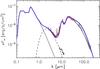 |
Fig. 4 Spectral energy distribution of HD 100546. Plotted in gray are the ISO spectrum (Malfait et al. 1998) and the stellar photosphere (van den Ancker et al. 1998). Plotted in black is the “inner disk spectrum” (the correlated spectrum of the 41.4 m baseline) and a 1700 K black body scaled to the K-band flux (dashed line). The colored lines show the same models as Fig. 1. The model without a gap is not shown. |
3. Deriving the wall shape
In this section we constrain the shape of the surface density profile in the disk wall from the visibilities presented by Panić et al. (2012) and Leinert et al. (2004). To do so, we need to first calculate the density and temperature structure in the disk wall for a given surface density profile. Because the structure of a rounded disk wall can strongly deviate from that of a geometrically thin disk, this task is especially well-suited for 2D radiative transfer codes – also because the disk wall near the midplane is completely shadowed by the inner disk, while the upper part is fully illuminated. In addition, we need to calculate the vertical structure in the disk wall, which strongly deviates from that of a continuous disk due to radial and vertical temperature gradients.
We used MCMax (Min et al. 2009), a 2D radiative transfer code that self-consistently calculates the temperature and vertical density structure for a given surface density profile in an axisymmetric geometry. We assumed the gas to be in vertical hydrostatic equilibrium, and because the SED shows no sign of dust settling of small grains (Mulders et al. 2013), we assume the dust and gas distributions to be equal. The SED and visibilities were calculated using ray-tracing to compare them with the observations. We used the SED fit with a vertical wall presented in Mulders et al. (2011) as a starting point, refined it using the constraints from Panić et al. (2012), and fit the SED and visibilities simultaneously to constrain the surface density in the disk wall. For completeness, all model parameters are displayed in Table 1.
Model parameters.
To generate visibilities from the observed correlated fluxes, we need to divide them by an observed total flux. Because the total flux measured with MIDI is affected by flux losses from the MIDI slit (see Panić et al. 2012), we used the flux measured with ISO to generate visibilities. The larger field of view of ISO also includes more large-scale PAH emission, with narrow features around 7.9, 8.6 and 11.3 μm, which are inversely imprinted in the visibilities, but which we did not model. These visibilities, together with those presented by Leinert et al. (2004), are shown in Fig. 5. We used the position angle of 145° and inclination of 53° derived by Panić et al. (2012) to compute visibilities from our disk models.
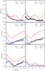 |
Fig. 5 Observed visibilities for HD 100546 on different projected baseline lengths and orientations (diamonds). We used the total flux from ISO to calculate visibilities from the correlated fluxes. The colored lines show the same models as Fig. 1. The model without a gap is not shown. |
3.1. Inner disk
As shown by Panić et al. (2012), the inner disk is – at least in the small dust grains probed by MIDI – very compact, <0.7 AU . This is perhaps best illustrated by plotting the correlated flux on the 41 m baseline into the SED of Fig. 4. This baseline probes scales about 2 to 3 AU and therefore filters out most of the emission from the outer disk. The correlated flux seems consistent with the 1700 K blackbody emission from the inner rim, with only little additional flux from colder material. We placed the inner rim at 0.25 AU, consistent with the near-infrared interferometric constrains from Benisty et al. (2010) and Tatulli et al. (2011). Because the temperature behind the inner rim at 0.25 AU drops off very rapidly with radius, we found that the inner disk cannot extend farther out than 0.3 AU (in small grains), unless the surface density power law is steeper than r-1. This tiny inner disk is similar to that in the transitional disk T Cha (Olofsson et al. 2013). The normalization of the surface density (Σinner) was fitted to the near-infrared excess.
In addition, there is a weak feature apparent at 10 micron, though it is not clear whether this is a mineralogical feature in the inner disk or due to the structure of the outer disk. The outer disk wall also contributes to the correlated flux and creates similar features – which we discuss extensively in the next section. If we treat the observed feature strength as an upper limit to the real feature strength, the feature is too weak to be consistent with a rim made out of the same small amorphous silicate grains as the outer disk wall. Because the temperature of the inner rim is higher than the crystallisation temperature of silicates – and possibly also higher than its sublimation temperature – we used a composition of pure iron, which also fits the SED (Fig. 4). We can mix in a few percent of silicates or corundum (FeAl2O3, which has a higher sublimation temperature) to fit the weak 10 micron feature in the correlated spectrum, but this is not required for a good fit to the visibilities and has no effect on the results presented in this paper.
3.2. Vertical wall
As explained in Sect. 2, the presence of a disk wall creates structures in the visibility as a function of baseline, which is reflected in the spectrally resolved visibilities as well (Fig. 5). This is most clearly seen in the 14.9 m baseline, where a bounce is present at 10.5 μm. Bounces are also present around 8.5 μm in the 15.8 and 16.0 m baselines. The longer baselines do not show such pronounced structures.
A disk model with a vertical wall at 14 AU can reproduce the location of these bounces at the shortest baselines (Fig. 5, red lines). However, this model overestimates the visibilities at these baselines. In addition, the vertical wall model predicts structures at the 41 and 74 m baselines that are not observed. To fit the visibilities at all baselines, we rounded off the disk wall as described in Sect. 2. This reduces the power in the sidelobes, thus reducing the visibilities at the shortest baselines and smoothing out structures at the longer baselines.
3.3. Rounded-off wall
We rounded off the disk wall by modifying its surface density power law using the following function: 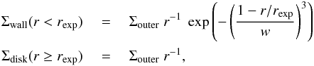 (1)where Σouter is the normalization constant for the outer disk surface density fitted to the SED, rexp is the radius where the drop-off of the surface density sets in, and w is a measure of how round the disk wall is. This function is essentially a Gaussian similar to the vertical scale height, but with a different exponent of 3 as in Lubow & D’Angelo (2006), Eq. (5). Both w and rexp are free fitting parameters. Examples of the resulting surface density distributions are shown in Fig. 2. Although different parametrizations than the one introduced here are possible, this particular one was chosen because it also accurately describes the outcome of our hydrodynamical simulations in the next section.
We first rounded off the disk wall using w = 0.20 and rexp = 19 AU (Fig. 2, red dotted line), consistent with the shape of the disk wall as modeled by Tatulli et al. (2011). Although this produces a smoother surface brightness profile than a vertical wall (Fig. 3) with less power in its sidelobes (Fig. 1), it still produces too much structure on the 41 and 74 meter baselines and overpredicts the shortest baselines. To completely remove all structure on the longer baselines, we rounded off the disk wall even more. Our best-fit model has w = 0.36 and rexp = 29 AU, shown by the blue lines in Figs. 1−3, and 5. There is a small range of solutions with almost equally good fits, ranging from w = 0.33 and rexp = 26 AU to w = 0.40 and rexp = 35 AU. The total parameter space explored ranges from w = 0.00 to w = 0.60, and from rexp = 10 to 40 AU.
We note that due to disk asymmetries and variability, as discussed by Panić et al. (2012), it is impossible to find a perfect fit to all data with a single axisymmetric model. Especially the 8 to 9 μm region dominated by the inner disk is affected by this, as observations taken at the same projected baseline length and position angle but at a different date have a different shape. However, the structures arising from vertical walls are not seen in any of the observations, so we are confident that our results for the wall shape are robust. Fitting each baseline separately does provide better fits, but does not change our fit parameters by more than Δw = 0.02 and Δrexp = 2 AU.
4. Deriving planet mass and disk viscosity
In this section, we show how a planet can explain the observed shape of the disk wall. The micron sized-dust grains observed with MIDI are a good tracer of the gas: they are well-coupled to the gas (Mulders et al. 2013, their Sect. 4.2), unlike millimeter sized grains, which tend to pile up near pressure bumps in the midplane (Paardekooper & Mellema 2004; Pinilla et al. 2012). Therefore, the inferred surface density of the dust is equal to that of the gas, which we reproduced using planet-disk interactions.
4.1. Gap opening
A planet embedded in a disk opens a gap by exerting a torque on the disk, pushing material outside of its orbit outward and material inside of it inward. However, gas flows back into the gap due to pressure gradients and viscous spreading, which tends to close the gap. Therefore, the shape of the surface density around a planet depends on its mass, the disk viscosity and scale height (Crida et al. 2006; Lubow & D’Angelo 2006). In general, a heavier planet can carve out a deeper and wider gap, while a more viscous or thicker disk (higher pressure scale height) will reduce the gap width and depth.
4.2. Hydrodynamical model
We used the freely available 2D hydrodynamical code Fargo (Masset 2000) to model the surface density of the gas disk around an embedded planet’s orbit. Fargo is a solver to the Navier-Stokes and continuity equations in a differentially rotating disk in vertical hydrostatic equilibrium. It speeds up these calculations by removing the average azimuthal velocity component from these equations at each radius and at each time-step.
Because we focused on the steady-state wall shape, it is not necessary to follow the global evolution of the whole disk as Tatulli et al. (2011) have done. Instead, we focused on the surface density profile in the vicinity of the planet. We modeled the disk within a factor 5 in radius of the planet (i.e., 2 to 50 AU for a planet at 10 AU), far enough from the grid edges so that their location do not affect the shape of the surface density in the vicinity of the planet. The planetary candidate discovered by Quanz et al. (2013) lies outside this grid, and – assuming it is on a circular orbit – is therefore located too far away to influence the gap structure. We used square grid cells on a logarithmic grid, 384 in the azimuthal direction. We used a non-reflective boundary condition to suppress wave-reflection at the inner boundary and prevent mass from leaking out at the inner edge of the grid.
The model set-up is based on our best-fit radiative transfer model to the SED and visibilities. We used a surface density power law of r-1 for the initial surface density, similar to that of the outer disk. We used a pressure scale height derived from the scale height profile of our radiative transfer simulation from within the disk gap, i.e., between 0.3 and ~13 AU. Because our radiative transfer model is not vertically isothermal, the scale height is defined as the height above the midplane where the pressure drops off by e− 1/2. The pressure scale height in this regime is well-fitted by a power law of the form Hp(r) = 0.025 r1.39, see also Fig. 9. We return to the influence of the chosen scale height profile in the discussion (Sect. 5.3).
To describe the viscous evolution of the disk, we used a viscosity of α type (Shakura & Sunyaev 1973; Pringle 1981), consistent with our choice of r-1 for the initial surface density profile. For the long integration times required to reach a steady state, this viscosity agrees well with simulations of magnetohydrodynamical turbulence (Papaloizou et al. 2004). We explored the range from α = 10-4 to α = 5 × 10⁻², above which the time step calculation of Fargo may no longer be correct.
We considered a wide range of planets from 1 Jupiter mass to the hydrogen-burning limit at 80 Jupiter masses. The reason for considering these high planet masses is that higher viscosities tend to close the gap, requiring much heavier planets to keep the gap open. We followed the disk evolution for 104 orbits of the planet around a 2.4 solar mass star (2 × 10⁵ yr at 10 AU), after which all models have reached a steady-state. The planet was assumed to be on a circular orbit, and to neither migrate, nor accrete3.
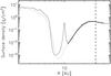 |
Fig. 6 Surface density around a 60-Jupiter-mass planet in a viscous (α = 2 × 10⁻²) disk after 104 orbits, with and without accretion onto the planet (dotted and solid gray line, respectively). The solid black line is the analytical fit using Eq. (1) with parameters that also fit the MIDI data (w = 0.36). The dashed line denotes rexp, the radius where the surface density starts to deviate from a power law. |
4.3. Gap shape
To compare the surface density profiles produced by Fargo with our radiative transfer models, we used the analytical fit function of Eq. (1). This function was fitted to the surface density profile outside the radial location of the planet, between rmin and rmax, where rmin is the location of the lowest gap depth outside the planets orbit (rmin > rp), and rmax is taken near the edge of the grid at 4.5rp. This radius was chosen to be just inside the outer grid edge, to avoid the region where the spiral wake hits this edge and local boundary effects may be important.
This function fits the surface density profiles with an accuracy of about 10%. An example is shown in Fig. 6. The main deviations come from transient features at small spatial scales, while the overall shape is generally well produced. Note that we did not use the results of the hydrodynamical simulation inside the planet’s orbit, and instead assumed this region to be empty, as indicated by our radiative transfer model, see Sect. 5.2 for a discussion on the gap width.
In addition, we measure the depth of the gap by taking the lowest density value with respect to the unperturbed density (Σouter r-1). Note that this is only a lower limit to the real depth of the gap: material that is corotating with the planet or orbits around it creates a surface density spike at the location of the planet. If planetary accretion is turned on, using the highest accretion efficiency following the prescription of Kley (1999), the spike disappears and the gap becomes deeper, typically by a factor of 2, though the shape of the disk wall at the far end of the gap does not change significantly, as shown by the dotted line in Fig. 6.
 |
Fig. 7 Shape of the disk wall as a function of planet mass and disk viscosity. Solid contours and colors denote the fitting parameter w from Eq. (1), which is w ∼0.33 to 0.40 for our best-fit radiative transfer models. The dashed line denotes a gap depth of 10-3. In the region below, the gap is deep enough to be consistent with the observed visibilities. Blue colors indicate rounder walls, red colors more vertical walls. The triangles indicate the models used for iterating on the pressure profile (see Sect. 5.3). The white regions contain models that neither converged nor finished 105 orbits due to excessive computing time. |
4.4. Results
The results of our parameter study are presented in Fig. 7, showing the width over which the surface density in the disk wall is rounded off (w from Eq. (1)) as a function of planet mass and disk viscosity. A general trend is visible, where lower planet masses and disk viscosities produce more vertical walls (w ~ 0.2), while rounder walls are found at higher values (w ~ 0.35). This trend can be understood from a balance between viscous spreading and planetary torques: a high viscosity makes material flow inward, which smoothes the surface density profile, while a heavier planet mass allows the torques to act over a wider range, allowing for a shallower profile. However, for intermediate shapes there is no linear trend (w ~ 0.25 to 0.3).
There is an additional observational constraint on the surface density profile, namely the depth of the gap (Tatulli et al. 2011). If the gap is not deep enough, its emission will fill the gap in the SED around 8 micron and will overpredict all visibilities. Because the inner disk is already depleted by a factor of a hundred, the gap needs to be depleted by about a factor of about ten more (see Fig. 2), depending on the dust opacities. This minimum gap depth is shown with the dashed line in Fig. 7, and only models below this line have gaps that are deep enough. It shows that the disk viscosity is a crucial parameter in opening a disk gap: a Jupiter-mass planet may open a deep gap in an inviscid disk, but for the most viscous disks it requires an 80-Jupiter-mass planet to keep the gap deep enough. In general, we find that the planet mass needs to be scaled with the square root of viscosity to achieve a given gap depth.
There are two regions in this diagram with a wall shape consistent with our observations, w ~ 0.33...0.40. One region lies at low planetary masses (<5 MJup) and high viscosities (α > 2 × 10⁻²). Although consistent with the planet mass estimate of Tatulli et al. (2011), the higher viscosity acts against gap opening, and these gaps are nowhere near deep enough to be consistent with observations, even if the planet were allowed to accrete. Another region lies at very high masses (30 to 80 MJup) and moderately high viscosities (α = 5 × 10⁻³ ... 5 × 10⁻²), which seems consistent with the observed gap depth, and puts the planet between 8 and 10 AU. Our best-fit model has a planet of 60 MJup at 10 AU, a viscosity of α = 2 × 10⁻², and is shown in Fig. 6. The dependence of these results on the assumed temperature profile is discussed in Sect. 5.3.
These estimates of α are consistent with that of Mulders et al. (2013), who also found a high turbulent mixing strength of αturb > 0.01 by considering the degree of dust settling in the disk wall.
5. Discussion
5.1. Planet or brown dwarf?
The shape of the disk wall points to a companion of thirty Jupiter masses or heavier, with a best fit at about 60 Jupiter masses. According to the IAU definition, this object would be a brown dwarf, and not a planet, making HD 100546 a misinterpreted binary system with a disk like CoKu Tau/4 (Ireland & Kraus 2008), rather than a transitional disk.
Binaries are common around main-sequence A stars and Herbig Ae/Be stars, with fractions over 70% (e.g. Baines et al. 2006; Kouwenhoven et al. 2007). The inferred period of around 20 years is consistent with the peak in the period distribution of binaries around sun-like stars (e.g. Zinnecker 1984; Raghavan et al. 2010). Whether a mass ratio of q ~ 0.02 is uncommon for binaries is not clear, because detection limits typically reach q ~ 0.1, but Wheelwright et al. (2010) noted that the companion distribution of Herbig Ae/Be companions is skewed toward higher masses than the interstellar mass function. However, we note that the companion candidate recently discovered around HD 142527 by Biller et al. (2012) has a very similar mass and orbital properties. In addition, there seems to be a trend from direct imaging that A-type stars posses heavier planets than less massive stars (Marois et al. 2008; Lagrange et al. 2010; Carson et al. 2013), a trend also seen in radial velocity surveys (Lovis & Mayor 2007).
Whether to call a companion a planet or a brown dwarf should depend on how it forms, not on its mass. Young stars are found with masses below the deuterium-burning limit (e.g. Luhman et al. 2005), while core-accretion models predict that planets can also form above it (Mordasini et al. 2009). A better definition would involve whether the formation process of the companion occured in a disk or like a single star. The current gas mass of the disk is uncertain due to lack of resolved millimeter observations, but is estimated to be in the range 0.0005 to 0.01 M⊙ (Panić et al. 2010; Thi et al. 2011) and therefore much lighter than the planet, making it unlikely that the planet recently formed out of the disk.
Observational limits exist on the mass and location of possible binary companions of HD 100546. Baines et al. (2006) reported no detection in a spectroastrometric survey for binary companions, with a contrast limit of 6 mag and minimum separation of 0.1′′, excluding a companion with spectral type earlier than M64 outside of 10 AU. Limits also exist on a companion in the gap: Grady et al. (2005) used UV spectroscopy to put an upper limit to the spectral type later than M5, excluding a stellar companion, but not a brown dwarf.
The projected location of the planet (0.05..0.1′′) is just inside the region that can be surveyed with current direct-imaging instruments (Quanz et al. 2011), and also falls within the region blocked by coronagraphs of upcoming planet-hunting instruments such as VLT/SPHERE and the Gemini Planet Imager. However, it is within the reach of techniques such as Sparse Aperture Masking (e.g. Kraus & Ireland 2012; Biller et al. 2012). We estimated the contrast ratio using the Baraffe et al. (2002) evolutionary tracks. A 20 to 75 Jupiter mass brown dwarf with an age younger than 10 Myr has a luminosity between 0.03 and 0.3 L⊙ and a temperature between 2500 and 3000 K. In the H, K, and L band, this results in a contrast ratio between 5 × 10⁻⁴ to 1 × 10⁻², or 5 to 8 mag, within the detectable range.
5.2. Gap width
The width of the gap from the hydrodynamical simulations, about 6 AU, is inconsistent with the derived size for the inner disk of less than one AU. The planet itself is heavier than the disk and probably does not migrate, allowing it to act as a barrier for material from the outer disk to reach the inner disk. We neglected the global evolution of the disk, so it is possible that in reality, the inner disk drains onto the central star as in Tatulli et al. (2011). The near-infrared interferometric data used by the authors, however, do not directly constrain the outer radius of the inner disk, which they placed at 4 AU. The MIDI data do require the inner disk to be much smaller than the 4 AU previously assumed (see also Panić et al. 2012). Therefore, an additional mechanism might be necessary for clearing the inner regions.
Additional planets closer to the star could explain the extent of the gap, because they might deplete the inner regions (Dodson-Robinson & Salyk 2011; Zhu et al. 2011). Because the torques on the disk are strongest close to a planet, we expect only the outermost planet in the gap to shape the disk wall. Another mechanism could be dust filtration at the outer edge, which would block dust particles from crossing the gap together with the gas and would reduce the dust to gas ratio of the inner disk (Zhu et al. 2012). However, the high viscosities we infer are less favorable for trapping dust in the outer disk wall (Pinilla et al. 2012). In addition, grain growth could contribute to depleting the inner disk of small grains, see Birnstiel et al. (2012). Resolved millimeter observations of the gap, such as can be delivered with the Atacama Large Millimeter Array, will be crucial to investigate this.
5.3. Pressure scale height
As mentioned in Sect. 4.1, the disk thickness – set by the pressure scale height and thus by temperature – is an important factor in determining the wall shape because it controls how much material flows back into the gap. The pressure scale height is an input parameter of Fargo and remained fixed during the simulation. This is a highly idealized situation, and in reality, the scale height will change during gap opening when the disk wall heats up (Turner et al. 2012). This will, in turn, influence the gap structure, but coupling the hydrodynamical simulations to radiative transfer is far from trivial. In this section we describe how this coupling may affect our results and suggest directions for future work.
Because we are looking for a steady-state solution of the wall shape after many orbits, we can derive the scale height profile corresponding to this wall shape from our best-fit radiative transfer model to the SED and visibilities. This profile is shown in Fig. 8. In the region up to ~12 AU, i.e., within the disk gap, the vertical optical depth is so low that the midplane is not shielded, increasing the temperature by a factor of two and the pressure scale height by about 50% with respect to a disk without a gap (dashed line, see also Turner et al. 2012). Between ~12 and 30 AU, the gradual increase in optical depth starts to shield the midplane, leading to lower temperatures and scale height. Outside 30 AU, the scale height profile is close to that of a continuous disk.
In the parameter study, we used a parameterized scale height of the form Hp(r) = 0.025 r1.39 (Fig. 8, dotted line). This parametrization describes the profile accurately up to ~12 AU, i.e., in most of the region modeled with Fargo. In addition, in the region where the intensity profile peaks (see Fig. 3) and where our observations are most sensitive, it is closer to the scale height of the best-fit radiative transfer model than that of a continuous disk is. However, the slope of the scale height profile after the peak in intensity at ~12 AU is very different. In a steady-state viscous disk without a gap, this slope sets the surface density distribution (e.g. Andrews et al. 2009). To see how this assumption affects our results, we designed the test described below.
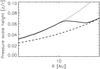 |
Fig. 8 Scale height profile for our best-fit radiative transfer model (solid line) in the range modeled with Fargo. Also plotted are the best-fit profile in the gap (Hp(r) = 0.025 r1.39, dotted line) and that of a disk without a gap (Hp(r) = 0.02 r1.32, dashed line). Because the radiative transfer model is not vertically isothermal, the scale height is defined as the height where the pressure drops off with a factor e1/2 with respect to the midplane. |
Wall shape and location before and after iterating on the temperature structure.
We performed one iteration on the hydrodynamical structure of the disk to take into account the change in temperature structure of the disk after gap opening. We started with a subset of the hydrodynamical models presented in the previous section, shown in Table 2 and indicated by triangles in Fig. 7. These models span the entire range of wall shapes, from steep to rounded-off, and were initially calculated using the parameterized scale height profile. For each wall shape w, we calculated the temperature structure using our radiative transfer code, as described in Sect. 3. The radial location of the wall depends – in addition to the planets location – also on the planet mass, because more massive planets carve out wider gaps. Therefore we adjusted the location of the planet rpl – and hence that of the disk wall (rexp, Eq. (1)) – to ensure that the radial intensity profile peaks at 12−13 AU for each wall shape, as in Fig. 3. This is equivalent to fitting the SED (but not the visibilities), since that only depends on the wall location, not its shape.
From these temperature structures we can calculate the scale height profiles, similar to Fig. 8. We used these (nonparameterized) profiles to rerun the hydrodynamical simulations, and measured the new wall shapes of these iterated models using Eq. (1). If the resulting radial location of the wall differs from that of the radiative transfer simulation, we reran the hydrodynamical simulation with the planet at a different radius, to ensure that the wall location between the two simulations is self-consistent. The wall shapes and location before and after iteration are shown in Table 2.
For walls that were already quite round before iterating on the scale height profile (M > 30 MJup and α > 5 × 10⁻³), using the calculated scale height from the radiative transfer model does not affect the wall shape significantly. For lower planet masses and disk viscosities, corresponding to steep walls before iteration, the wall shape does change. Iterating on the pressure profile makes these walls rounder by Δw = 0.04 to 0.07. An example of this is shown in Fig. 9, for a 20-Jupiter-mass planet in a moderately viscous disk (α = 2 × 10⁻³). By looking at Fig. 7, this moves down the lower limit on the possible range of planet masses and disk viscosities from 30 to 20 Jupiter masses and from α = 5 × 10⁻³ to 2 × 10⁻³, respectively, becoming consistent with the estimates of Acke & van den Ancker (2006).
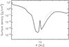 |
Fig. 9 Surface density around a 20-Jupiter-mass planet in a viscous (α = 2 × 10⁻³) disk for two different temperature profiles. The dotted line has a power-law scale height profile resulting in a steep wall (w = 0.26), the solid line uses the scale height profile from the radiative transfer calculation, resulting in a rounder wall (w = 0.32). |
We show that iterating on the scale height profile in hydrodynamical simulations does affect the resulting wall shapes. However, we did not take the feedback of the disk structure on the pressure profile during the gap opening into account. To do this, one would need to recalculate the scale height profile during the hydrodynamical calculation, such that the wall shape and scale height profile are always self-consistent. However, this approach is clearly beyond the scope of this paper. We leave this for future work, but we do note that the temperature structure in the wall may contribute to its roundness and might play a role in other processes relevant to transitional disks, such as the accretion flow across the gap. Ideally, one would also take into account the 3D structure of the wall, though this might take a considerable computational effort due to the long integration times necessary to reach a steady state.
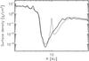 |
Fig. 10 Comparison of the radial surface density profile (black line) with the azimuthally averaged one (gray line), for our best-fit model of Fig. 6. |
5.4. Gap eccentricity
Throughout this work, we assumed azimuthal symmetry for the disk. However, toward the highest companion masses in our simulations, the gap starts to become eccentric (see also Casassus et al. 2012). In addition, the chromatic phases measured with MIDI also show indications for an asymmetric outer disk (Panić et al. 2012). Taking an azimuthal average over an eccentric gap can lead to a rounder surface density profile, but we will show that this is not the effect we observe or measure in our simulations.
From a modeling point of view, making a gap eccentric contributes to the roundness measured from an azimuthally averaged surface density profile under certain conditions. For example, an elliptical gap (e = 0.4) with a vertical wall has an azimuthally averaged surface density profile that appears to be slightly rounded off (we fit w = 0.05). This is much less round than the lowest roundness we measured in our simulations, which is w = 0.17 (for a circular gap). To investigate if the eccentricity may contribute to the inferred roundness we compared radial cuts of the surface density profile with azimuthally averaged ones. An example is shown in Fig. 10 for our best-fit model, which has an eccentricity of e ≈ 0.6. The radial cut is significantly more noisy – motivating the use of azimuthally averaged profiles – but the shape of the wall does not change significantly, although it is radially displaced by a few AU.
From an observational perspective, the eccentricity of the gap does not change the roundness of the disk wall, as inferred from the visibilities. Each visibility is measured along a particular baseline orientation and is therefore sensitive to the radial gradient of the surface density along that baseline, without any azimuthal averaging. The radial displacement of the disk wall due to eccentricity is measurable, but unfortunately this effect is degenerate with disk inclination and position angle, increasing the uncertainties on these parameters.
It may be possible to constrain the eccentricity from the the chromatic phases, hence providing an extra diagnostic on the companion mass, but this will require in-depth modeling of a more extended data set.
6. Conclusion
We have studied the gap shape in the disk of HD 100546. By comparing 2D radiative transfer models to the mid-infrared interferometric data presented in Panić et al. (2012), we found that:
-
The disk wall at the far end of the gap is not vertical, but rounded offover a significant radial range. This shape can be explained by agradual increase in the surface density over a range of ~10 to ~25 AU, creating a broad peak in the surface brightness profile around 12 AU that was also seen by Panić et al. (2012).
-
The inner dust disk is extremely small in small grains. We confirmed the upper limit on its size of 0.7 AU found by Panić et al. (2012) and used our 2D radiative transfer model to constrain it even further, with no measurable contribution outside of 0.3 AU.
-
The roundness or spatial extent of a disk wall can be inferred from spectrally resolved visibilities beyond the first null.
By comparing these results with hydrodynamical simulations of planet-disk interactions, we found that:
-
The shape of the surface density profile in the disk wall of HD100546 can be explained by a massive planet (≳30...80 MJup) in a viscous (α ≳ 5 × 10⁻³) disk between 8 and 10 AU.
-
The roundness of a disk wall in hydrodynamical simulations depends on the temperature structure in the disk wall: iterating on the scale height profile using radiative transfer changes this roundness.
-
The disk viscosity is a crucial parameter in estimating planet masses from a derived surface density profile, acting against gap opening by the planet. For a given depth, the gap-opening mass of a planet increases with the square root of the disk’s viscosity.
-
The effect of a single planet is not enough to explain the full width of the disk gap in HD 100546. Either an additional clearing mechanism or a multi-planet system is required to explain its extent.
-
The object shaping the disk wall is most likely a brown dwarf, suggesting HD 100546 might be a binary system and not a transitional disk object.
At the time of writing, there are no published observations that constrain the gap size at (sub)millimeter wavelengths.
Assuming the inner and outer radius of the disk lie outside the emitting region, so there is no discontinuity in surface brightness at any radius.
With the exception of the model represented by the dotted line in Fig. 6, which uses the highest accretion efficiency as defined in Kley (1999).
Calculated at 5 Myr using the evolutionary tracks from Siess et al. (2000).
Acknowledgments
This research project is financially supported by a joint grant from the Netherlands Research School for Astronomy (NOVA) and the Netherlands Institute for Space Research (SRON). The work of O.P. was supported by the European Union through ERC grant number 279973.
References
- Acke, B., & van den Ancker, M. E. 2006, A&A, 449, 267 [NASA ADS] [CrossRef] [EDP Sciences] [Google Scholar]
- Andrews, S. M., Wilner, D. J., Hughes, A. M., Qi, C., & Dullemond, C. P. 2009, ApJ, 700, 1502 [NASA ADS] [CrossRef] [Google Scholar]
- Andrews, S. M., Wilner, D. J., Espaillat, C., et al. 2011, ApJ, 732, 42 [NASA ADS] [CrossRef] [Google Scholar]
- Ardila, D. R., Golimowski, D. A., Krist, J. E., et al. 2007, ApJ, 665, 512 [NASA ADS] [CrossRef] [Google Scholar]
- Baines, D., Oudmaijer, R. D., Porter, J. M., & Pozzo, M. 2006, MNRAS, 367, 737 [NASA ADS] [CrossRef] [MathSciNet] [Google Scholar]
- Baraffe, I., Chabrier, G., Allard, F., & Hauschildt, P. H. 2002, A&A, 382, 563 [NASA ADS] [CrossRef] [EDP Sciences] [Google Scholar]
- Benisty, M., Tatulli, E., Menard, F., & Swain, M. R. 2010, A&A, 511, A75 [NASA ADS] [CrossRef] [EDP Sciences] [Google Scholar]
- Biller, B., Lacour, S., Juhász, A., et al. 2012, ApJ, 753, L38 [NASA ADS] [CrossRef] [Google Scholar]
- Birnstiel, T., Andrews, S. M., & Ercolano, B. 2012, A&A, 544, A79 [NASA ADS] [CrossRef] [EDP Sciences] [Google Scholar]
- Bouwman, J., de Koter, A., Dominik, C., & Waters, L. B. F. M. 2003, A&A, 401, 577 [NASA ADS] [CrossRef] [EDP Sciences] [Google Scholar]
- Brittain, S. D., Najita, J. R., & Carr, J. S. 2009, ApJ, 702, 85 [NASA ADS] [CrossRef] [Google Scholar]
- Brown, J. M., Blake, G. A., Qi, C., et al. 2009, ApJ, 704, 496 [NASA ADS] [CrossRef] [Google Scholar]
- Calvet, N., D’alessio, P., Watson, D. M., et al. 2005, ApJ, 630, L185 [NASA ADS] [CrossRef] [Google Scholar]
- Carson, J., Thalmann, C., Janson, M., et al. 2013, ApJ, 763, L32 [NASA ADS] [CrossRef] [Google Scholar]
- Casassus, S., Perez, M. S., Jordán, A., et al. 2012, ApJ, 754, L31 [NASA ADS] [CrossRef] [Google Scholar]
- Crida, A., Morbidelli, A., & Masset, F. 2006, Icarus, 181, 587 [Google Scholar]
- de Val-Borro, M., Edgar, R. G., Artymowicz, P., et al. 2006, MNRAS, 370, 529 [NASA ADS] [CrossRef] [Google Scholar]
- Dodson-Robinson, S. E., & Salyk, C. 2011, ApJ, 738, 131 [CrossRef] [Google Scholar]
- Dorschner, J., Begemann, B., Henning, T., Jaeger, C., & Mutschke, H. 1995, A&A, 300, 503 [NASA ADS] [Google Scholar]
- Dullemond, C. P., & Monnier, J. D. 2010, ARA&A, 48, 205 [NASA ADS] [CrossRef] [Google Scholar]
- Grady, C. A., Woodgate, B., Heap, S. R., et al. 2005, ApJ, 620, 470 [Google Scholar]
- Henning, T., & Stognienko, R. 1996, A&A, 311, 291 [NASA ADS] [Google Scholar]
- Huelamo, N., Figueira, P., Bonfils, X., et al. 2008, A&A, 489, L9 [NASA ADS] [CrossRef] [EDP Sciences] [Google Scholar]
- Ireland, M. J., & Kraus, A. L. 2008, ApJ, 678, L59 [NASA ADS] [CrossRef] [Google Scholar]
- Juhász, A., Bouwman, J., Henning, T., et al. 2010, ApJ, 721, 431 [NASA ADS] [CrossRef] [Google Scholar]
- Kley, W. 1999, MNRAS, 303, 696 [NASA ADS] [CrossRef] [Google Scholar]
- Kouwenhoven, M. B. N., Brown, A. G. A., Portegies Zwart, S. F., & Kaper, L. 2007, A&A, 474, 77 [NASA ADS] [CrossRef] [EDP Sciences] [Google Scholar]
- Kraus, A. L., & Ireland, M. J. 2012, ApJ, 745, 5 [NASA ADS] [CrossRef] [Google Scholar]
- Lagrange, A. M., Bonnefoy, M., Chauvin, G., et al. 2010, Science, 329, 57 [NASA ADS] [CrossRef] [PubMed] [Google Scholar]
- Leinert, C., van Boekel, R., Waters, L. B. F. M., et al. 2004, A&A, 423, 537 [NASA ADS] [CrossRef] [EDP Sciences] [Google Scholar]
- Lin, D. N. C., & Papaloizou, J. 1979, MNRAS, 186, 799 [NASA ADS] [CrossRef] [Google Scholar]
- Lin, D. N. C., & Papaloizou, J. 1986, ApJ, 307, 395 [NASA ADS] [CrossRef] [Google Scholar]
- Liu, W. M., Hinz, P. M., Meyer, M. R., et al. 2003, ApJ, 598, L111 [NASA ADS] [CrossRef] [Google Scholar]
- Lovis, C., & Mayor, M. 2007, A&A, 472, 657 [NASA ADS] [CrossRef] [EDP Sciences] [Google Scholar]
- Lubow, S. H., & D’Angelo, G. 2006, ApJ, 641, 526 [NASA ADS] [CrossRef] [Google Scholar]
- Luhman, K. L., Adame, L., D’Alessio, P., et al. 2005, ApJ, 635, L93 [NASA ADS] [CrossRef] [Google Scholar]
- Malfait, K., Waelkens, C., Waters, L. B. F. M., et al. 1998, A&A, 332, L25 [NASA ADS] [Google Scholar]
- Marois, C., Macintosh, B., Barman, T., et al. 2008, Science, 322, 1348 [NASA ADS] [CrossRef] [PubMed] [Google Scholar]
- Masset, F. S. 2000, in Disks, Planetesimals, and Planets, ASP Conf. Proc., 219, 75 [Google Scholar]
- Min, M., Dullemond, C. P., Dominik, C., de Koter, A., & Hovenier, J. W. 2009, A&A, 497, 155 [NASA ADS] [CrossRef] [EDP Sciences] [Google Scholar]
- Mordasini, C., Alibert, Y., & Benz, W. 2009, A&A, 501, 1139 [NASA ADS] [CrossRef] [EDP Sciences] [Google Scholar]
- Mulders, G. D., Waters, L. B. F. M., Dominik, C., et al. 2011, A&A, 531, A93 [NASA ADS] [CrossRef] [EDP Sciences] [Google Scholar]
- Mulders, G. D., Min, M., Dominik, C., Debes, J. H., & Schneider, G. 2013, A&A, 549, A112 [NASA ADS] [CrossRef] [EDP Sciences] [Google Scholar]
- Mutschke, H., Begemann, B., Dorschner, J., et al. 1998, A&A, 333, 188 [NASA ADS] [Google Scholar]
- Muzerolle, J., D’Alessio, P., Calvet, N., & Hartmann, L. 2004, ApJ, 617, 406 [NASA ADS] [CrossRef] [Google Scholar]
- Olofsson, J., Benisty, M., Le Bouquin, J.-B., et al. 2013, A&A, 552, A4 [NASA ADS] [CrossRef] [EDP Sciences] [Google Scholar]
- Paardekooper, S. J., & Mellema, G. 2004, A&A, 425, L9 [NASA ADS] [CrossRef] [EDP Sciences] [Google Scholar]
- Panić, O., van Dishoeck, E. F., Hogerheijde, M. R., et al. 2010, A&A, 519, A110 [NASA ADS] [CrossRef] [EDP Sciences] [Google Scholar]
- Panić, O., Ratzka, T., Mulders, G. D., et al. 2012, A&A, submitted [arXiv:1203.6265] [Google Scholar]
- Papaloizou, J. C. B., Nelson, R. P., & Snellgrove, M. D. 2004, MNRAS, 350, 829 [NASA ADS] [CrossRef] [Google Scholar]
- Pinilla, P., Benisty, M., & Birnstiel, T. 2012, A&A, 545, A81 [NASA ADS] [CrossRef] [EDP Sciences] [Google Scholar]
- Preibisch, T., Ossenkopf, V., Yorke, H. W., & Henning, T. 1993, A&A, 279, 577 [NASA ADS] [Google Scholar]
- Pringle, J. E. 1981, ARA&A, 19, 137 [NASA ADS] [CrossRef] [Google Scholar]
- Quanz, S. P., Schmid, H. M., Geissler, K., et al. 2011, ApJ, 738, 23 [NASA ADS] [CrossRef] [Google Scholar]
- Quanz, S. P., Amara, A., Meyer, M. R., et al. 2013, ApJ, 766, L1 [NASA ADS] [CrossRef] [Google Scholar]
- Raghavan, D., McAlister, H. A., Henry, T. J., et al. 2010, ApJS, 190, 1 [NASA ADS] [CrossRef] [EDP Sciences] [Google Scholar]
- Ratzka, T., Leinert, C., Henning, T., et al. 2007, A&A, 471, 173 [NASA ADS] [CrossRef] [EDP Sciences] [Google Scholar]
- Setiawan, J., Henning, T., Launhardt, R., et al. 2008, Nature, 451, 38 [NASA ADS] [CrossRef] [PubMed] [Google Scholar]
- Shakura, N. I., & Sunyaev, R. A. 1973, A&A, 24, 337 [NASA ADS] [Google Scholar]
- Siess, L., Dufour, E., & Forestini, M. 2000, A&A, 358, 593 [NASA ADS] [Google Scholar]
- Steinacker, J., & Henning, T. 2003, ApJ, 583, L35 [NASA ADS] [CrossRef] [Google Scholar]
- Strom, K. M., Strom, S. E., Edwards, S., Cabrit, S., & Skrutskie, M. F. 1989, AJ, 97, 1451 [NASA ADS] [CrossRef] [Google Scholar]
- Tannirkulam, A., Monnier, J. D., Harries, T. J., et al. 2008, ApJ, 689, 513 [NASA ADS] [CrossRef] [Google Scholar]
- Tatulli, E., Benisty, M., Menard, F., et al. 2011, A&A, 531, A1 [NASA ADS] [CrossRef] [EDP Sciences] [Google Scholar]
- Thi, W. F., Menard, F., Meeus, G., et al. 2011, A&A, 530, L2 [NASA ADS] [CrossRef] [EDP Sciences] [Google Scholar]
- Turner, N. J., Choukroun, M., Castillo-Rogez, J., & Bryden, G. 2012, ApJ, 748, 92 [NASA ADS] [CrossRef] [Google Scholar]
- van den Ancker, M. E., The, P. S., Tjin A Djie, H. R. E., et al. 1997, A&A, 324, L33 [NASA ADS] [Google Scholar]
- van den Ancker, M. E., de Winter, D., & Tjin A Djie, H. R. E. 1998, A&A, 330, 145 [NASA ADS] [Google Scholar]
- Van Der Plas, G., van den Ancker, M. E., Acke, B., et al. 2009, A&A, 500, 1137 [NASA ADS] [CrossRef] [EDP Sciences] [Google Scholar]
- van Leeuwen, F. 2007, Hipparcos, the New Reduction of the Raw Data, Astrophys. Space Sci. Lib., 350 [Google Scholar]
- Varnière, P., Bjorkman, J. E., Frank, A., et al. 2006, ApJ, 637, L125 [NASA ADS] [CrossRef] [Google Scholar]
- Wheelwright, H. E., Oudmaijer, R. D., & Goodwin, S. P. 2010, MNRAS, 401, 1199 [NASA ADS] [CrossRef] [Google Scholar]
- Wolf, S., Moro-Martín, A., & D’Angelo, G. 2007, Planet. Space Sci., 55, 569 [NASA ADS] [CrossRef] [Google Scholar]
- Zhu, Z., Nelson, R. P., Hartmann, L., Espaillat, C., & Calvet, N. 2011, ApJ, 729, 47 [NASA ADS] [CrossRef] [Google Scholar]
- Zhu, Z., Nelson, R. P., Dong, R., Espaillat, C., & Hartmann, L. 2012, ApJ, 755, 6 [NASA ADS] [CrossRef] [Google Scholar]
- Zinnecker, H. 1984, IAU, 99, 41 [Google Scholar]
All Tables
All Figures
|
Fig. 1 Visibilities versus baseline length for HD 100546 at 10 micron, along a position angle of 30 degree (the same as the 41 meter baselines). The colored lines show a very round wall in blue, a steeper wall in dotted red, a vertical wall in solid red, and a model without a gap in dotted gray. Note that in the model without a gap the emission is coming from much closer to the star, and visibilities are much higher. Indicated in green are the spatial frequency ranges probed by the MIDI spectra used in this paper (λ = 8....13 micron), displayed as effective baseline at ten micron (Baseline/λ × 10 μm). |
| In the text | |
|
Fig. 2 Surface density profile of the disk for the same models as in Fig. 1. The surface density normalizations are those of the best-fit model described in Table 1. |
| In the text | |
|
Fig. 3 Radial brightness profile of the disk at 12.5 μm for the same models as in Fig. 1. The model without a gap has no brightness peak in this range and is not shown. |
| In the text | |
|
Fig. 4 Spectral energy distribution of HD 100546. Plotted in gray are the ISO spectrum (Malfait et al. 1998) and the stellar photosphere (van den Ancker et al. 1998). Plotted in black is the “inner disk spectrum” (the correlated spectrum of the 41.4 m baseline) and a 1700 K black body scaled to the K-band flux (dashed line). The colored lines show the same models as Fig. 1. The model without a gap is not shown. |
| In the text | |
|
Fig. 5 Observed visibilities for HD 100546 on different projected baseline lengths and orientations (diamonds). We used the total flux from ISO to calculate visibilities from the correlated fluxes. The colored lines show the same models as Fig. 1. The model without a gap is not shown. |
| In the text | |
|
Fig. 6 Surface density around a 60-Jupiter-mass planet in a viscous (α = 2 × 10⁻²) disk after 104 orbits, with and without accretion onto the planet (dotted and solid gray line, respectively). The solid black line is the analytical fit using Eq. (1) with parameters that also fit the MIDI data (w = 0.36). The dashed line denotes rexp, the radius where the surface density starts to deviate from a power law. |
| In the text | |
|
Fig. 7 Shape of the disk wall as a function of planet mass and disk viscosity. Solid contours and colors denote the fitting parameter w from Eq. (1), which is w ∼0.33 to 0.40 for our best-fit radiative transfer models. The dashed line denotes a gap depth of 10-3. In the region below, the gap is deep enough to be consistent with the observed visibilities. Blue colors indicate rounder walls, red colors more vertical walls. The triangles indicate the models used for iterating on the pressure profile (see Sect. 5.3). The white regions contain models that neither converged nor finished 105 orbits due to excessive computing time. |
| In the text | |
|
Fig. 8 Scale height profile for our best-fit radiative transfer model (solid line) in the range modeled with Fargo. Also plotted are the best-fit profile in the gap (Hp(r) = 0.025 r1.39, dotted line) and that of a disk without a gap (Hp(r) = 0.02 r1.32, dashed line). Because the radiative transfer model is not vertically isothermal, the scale height is defined as the height where the pressure drops off with a factor e1/2 with respect to the midplane. |
| In the text | |
|
Fig. 9 Surface density around a 20-Jupiter-mass planet in a viscous (α = 2 × 10⁻³) disk for two different temperature profiles. The dotted line has a power-law scale height profile resulting in a steep wall (w = 0.26), the solid line uses the scale height profile from the radiative transfer calculation, resulting in a rounder wall (w = 0.32). |
| In the text | |
|
Fig. 10 Comparison of the radial surface density profile (black line) with the azimuthally averaged one (gray line), for our best-fit model of Fig. 6. |
| In the text | |
Current usage metrics show cumulative count of Article Views (full-text article views including HTML views, PDF and ePub downloads, according to the available data) and Abstracts Views on Vision4Press platform.
Data correspond to usage on the plateform after 2015. The current usage metrics is available 48-96 hours after online publication and is updated daily on week days.
Initial download of the metrics may take a while.