| Issue |
A&A
Volume 557, September 2013
|
|
|---|---|---|
| Article Number | A86 | |
| Number of page(s) | 15 | |
| Section | Numerical methods and codes | |
| DOI | https://doi.org/10.1051/0004-6361/201220616 | |
| Published online | 06 September 2013 | |
Resolving galaxies in time and space
I. Applying STARLIGHT to CALIFA datacubes
1
Instituto de Astrofísica de Andalucía (CSIC),
PO Box 3004,
18080
Granada,
Spain
e-mail:
cid@astro.ufsc.br
2
Departamento de Física, Universidade Federal de Santa
Catarina, PO Box 476,
88040-900, Florianópolis, SC, Brazil
3
Centro Astronómico Hispano Alemán, Calar Alto, (CSIC-MPG), C/Jesús
Durbán Remón 2-2, 04004
Almería,
Spain
4
Leibniz-Institut für Astrophysik Potsdam,
innoFSPEC Potsdam, An der
Sternwarte 16, 14482
Potsdam,
Germany
5
Instituto de Astrofísica de Canarias, Vía Lactea s/n, 38200 La Laguna, Tenerife, Spain
6
Departamento de Astrofísica, Universidad de La
Laguna, 38205
Tenerife,
Spain
7
Departamento de Física Teórica, Universidad Autónoma de
Madrid, 28049
Madrid,
Spain
Received:
23
October
2012
Accepted:
16
April
2013
Aims. Fossil record methods based on spectral synthesis techniques have matured during the past decade, and their application to integrated galaxy spectra has fostered substantial advances in the understanding of galaxies and their evolution. Yet, because of the lack of spatial resolution, these studies are limited to a global view, providing no information about the internal physics of galaxies.
Methods. Motivated by the CALIFA survey, which is gathering integral field spectroscopy (IFS) over the full optical extent of 600 galaxies, we have developed an end-to-end pipeline that: (i) partitions the observed datacube into Voronoi zones in order to, when necessary and taking due account of correlated errors, increase the signal-to-noise ratio; (ii) extracts rest-framed spectra, including propagated errors and bad-pixel flags; (iii) feeds the spectra into the starlight spectral synthesis code; (iv) packs the results for all galaxy zones into a single FITS or HDF5 file; (v) performs a series of post-processing operations, including zone-to-pixel image reconstruction and unpacking the spectral and stellar population properties derived by starlight into multidimensional time, metallicity, and spatial coordinates. This paper provides an illustrated description of the whole pipeline and its many products. Using data for the nearby spiral NGC 2916 as a showcase, we go through each of the steps involved and present a series of ways of visualizing and analyzing this manifold. These include 2D maps of properties such as the velocity field, stellar extinction, mean ages and metallicities, mass surface densities, and star formation rates on different time scales and normalized in different ways, as well as 1D averages in the temporal and spatial dimensions, which lead to evolutionary curves and radial profiles of physical properties. Projections of the stellar light and mass growth onto radius-age diagrams are introduced as a means of visualizing galaxy evolution in time and space simultaneously, something which can also be achieved in 3D with snapshot cuts through the (x,y,t) cubes.
Results. The results vividly illustrate the richness both of the combination of IFS data with spectral synthesis and of the insights on galaxy physics provided by the variety of diagnostics and semi-empirical constraints obtained. Additionally, they give a glimpse of what is to come from CALIFA and future IFS surveys.
Key words: galaxies: general / galaxies: stellar content / galaxies: fundamental parameters
© ESO, 2013
1. Introduction
Technology in the past decade has lead to massive surveys either in imaging or spectroscopy modes that have been very successful in providing information of the spectral energy distribution or central/integrated spectra for a large number of galaxies (e.g., 2dF, Folkes et al. 1999; SDSS, York et al. 2000; COMBO-17, Bell et al. 2004; ALHAMBRA, Moles et al. 2008; COSMOS, Ilbert et al. 2009). These data have allowed significant insight into the integrated properties of galaxies, as well as into the evolution of global quantities such as the mass assembly (Pérez-Gonzalez et al. 2008) and the star formation history (SFH) of the universe (Lilly et al. 1996; Madau et al. 1996). However, these surveys are limited in either spectral or spatial resolution. Imaging provides spatial information, but at the expense of coarse spectral coverage (typically broadband filters), limiting the amount of information on the stellar populations, and providing little or no information on the gas (emission lines) or the kinematics of the galaxy. Surveys based on integrated spectra offer a richer list of diagnostics of the gaseous and stellar components but lack spatial resolution and suffer from aperture effects (one spectrum per object, centered at the nucleus and not covering the full galaxy). Moreover, integrated galaxy spectra do not allow, for example, the isolation of morphological components (bulge, disk, bars), the mapping of the effects of mergers, and the tracing of secular processes such as stellar migration and other features of galaxy formation and evolution, which can only be observationally tackled with a combination of imaging and spectroscopic capabilities.
The near future will see a proliferation of integral field spectroscopy (IFS) surveys, which will allow a detailed look at physics within galaxies, as opposed to the global view offered by integrated light surveys. The Calar Alto Legacy Integral Field Area survey (CALIFA) is a pioneer in this area (Sánchez et al. 2012), and others will follow soon, like SAMI (Croom et al. 2012), VENGA (Blanc et al. 2009), and MaNGA (Bundy et al., in prep.). CALIFA is obtaining IFS for 600 nearby galaxies (0.005 < z < 0.03) of all types, mapping stellar populations, ionized gas and their kinematics across the full optical extent of the sources. The number of spectra to be generated is of the same order of the whole SDSS (~106).
Clearly, however, these will not be “just another million galaxy spectra”. Processed through the machinery of fossil record methods, which recover the history of a stellar system out of the information encoded in its spectrum (Walcher et al. 2011 and references therein), CALIFA will provide valuable and hitherto unavailable information on the spatially resolved SFH of galaxies. An example of what can be done was presented by Pérez et al. (2012), where we used data on the first 105 galaxies observed by CALIFA in conjunction with the spectral synthesis code starlight (Cid Fernandes et al. 2005) to study the spatially resolved mass assembly history of galaxies. We find that the inner parts of massive galaxies grow faster than the outer ones, a clear signature of inside-out growth, and that the relative growth rate depends on the stellar mass of the galaxy, with a maximum relative growth efficiency for intermediate masses (~7 × 10¹⁰ M⊙).
The application of spectral synthesis methods to IFS datacubes opens new ways of studying galaxies and their evolution. In practice, however, this apparently simple extension of work done for spatially integrated spectra involves a series of technical details and methodological issues, as well as challenges in the visualization and representation of the results.
The purpose of this paper is to present a detailed account of all steps in the processing of CALIFA (x,y,λ) datacubes to the multidimensional products derived from the starlight analysis. We thus focus basically on methodology, leaving the exploration of results for subsequent studies. Paper II (Cid Fernandes et al. 2013) presents a thorough study of the uncertainties involved in these products, including the effects of random noise, spectral shape errors, and evolutionary synthesis models used in the analysis. Despite the emphasis on CALIFA and starlight, the issues discussed here and in Paper II are of direct interest to spectral synthesis analysis of IFS data in general.
The paper is organized as follows. Section 2 presents the data. Section 3 provides a detailed description of the pre-processing steps, which prepare the reduced data for a full spectral fitting analysis. Section 4 reviews the starlight code and the ingredients used in our analysis. It also introduces the PyCASSO pipeline, used to pack and analyze the results of the synthesis. Our main results are presented in Sect. 5, which uses the nearby spiral NGC 2916 (galaxy 277 in the CALIFA mother sample) as a showcase. This long section starts with considerations on how to evaluate the quality of the spectral fits, and then proceeds to the presentation of the synthesis products in different ways, including 2D maps of the stellar light and mass, extinction, mean ages and metallicities, and star formation rate maps on different time scales; 1D maps on either the spatial or temporal dimensions, and attempts to visualize the evolution of galaxies in time and space simultaneously. The emphasis is always on methodological issues, but the examples naturally illustrate the richness of the multidimensional products of this analysis. Finally, our results are summarized in Sect. 6.
2. Data
The goals, observational strategy and overall characteristics of the survey were described in Sánchez et al. (2012). In summary, CALIFA’s mother sample comprises 939 galaxies in the 0.005−0.03 redshift range, which is extracted from the SDSS imaging survey to span the full color−magnitude diagram down to Mr < −18 mag, with diameters selected to match the field of the IFU instrument (~1′ in diameter). A thorough characterization of the sample will be presented in Walcher et al. (in prep). CALIFA will observe ~600 galaxies from this mother sample, applying purely visibility-based criteria at each observing night. The final sample will be representative of galaxies in the local universe, statistically significant, and well selected.
The data analyzed in this paper were reduced using the CALIFA pipeline version 1.3c, described in the Data Release 1 article (Husemann et al. 2013). Each galaxy is observed with PMAS (Roth et al. 2005, 2010) in the PPAK mode (Verheijen et al. 2004; Kelz et al. 2006) at the 3.5 m telescope of Calar Alto Observatory and with two grating setups: the V500, covering from ~3700 to 7500 Å at FWHM ~ 6 Å resolution, and the V1200 (~3650−4600 Å, FWHM ~ 2.3 Å). The wide wavelength coverage of the V500 is ideal for our purposes, but the blue end of its spectra, which contains valuable stellar population tracers such as the 4000 Å break and high-order Balmer lines, is affected by vignetting over a non-negligible part of the field of view. To circumvent this problem we worked with a combination of the two gratings, whereby the data for λ < 4600 Å come from the V1200 (which does not suffer from this problem at this wavelength range) and the rest from the V500. The spectra were homogenized to the resolution of the V500.
For each galaxy the pipeline provides an (x,y,λ) cube with a final sampling of (1′′,1′′,2 Å). The cube comprises absolute calibrated flux densities at each spaxel (Fλ), corrected by Galactic extincion using the Schlegel et al. (1998) maps and the extinction law of Cardelliet al. (1989) law with RV = 3.1. Besides fluxes, the reduced cubes contain carefully derived errors (ϵλ) and a bad-pixel flag (bλ), which signals unreliable flux entries, due to bad columns, cosmic rays, and other artefacts (see Husemann et al. 2013, for details).
3. Pre-processing steps: from datacubes to STARLIGHT input
A series of pre-processing steps is applied to the reduced datacubes, with the general goal of extracting good quality spectra for a stellar population analysis with starlight or any other similar code. These are:
-
1.
definition of a spatial mask;
-
2.
outer signal-to-noise ratio (S/N) mask;
-
3.
refinements of the bλ (flag) and ϵλ (error) spectra;
-
4.
rest framing;
-
5.
spatial binning;
-
6.
resampling in λ.
3.1. Spatial masks
The first step is to mask out foreground stars, artefacts, and low S/N regions. As a starting point, candidate spurious sources are identified applying SExtractor (Bertin & Arnouts 1996) to the SDSS r-band image. The masked image is then matched to the CALIFA field of view using the WCS information available in the headers to reproject the SDSS masks to the scale, orientation, and pixel size of the CALIFA cubes. To improve upon this first approximation, we perform a visual inspection of each galaxy, correcting its mask interactively whenever necessary. For instance, we manually fixed a few unmasked pixels that remained in the borders of each masked object (probably due to a combination of the slightly better PSF of the SDSS images and the accuracy of the CALIFA WCS information used in the matching). Also, in a number of cases we found that the initial mask included bright Hii regions, while in others very dim point-like sources can be distinguished in the SDSS image, but have no clear counterpart in the CALIFA image or spectra. In all cases, the masks were corrected by hand.
The resulting masks are free from spurious spaxels. Unlike the other operations described below, this step could not be fully automated. For the size of CALIFA, this is still a feasible, albeit laborius, task. A last step in defining the spatial mask is to impose a spectral quality threshold based on the S/N of the data. This step has been fully automated in the pipeline described next.
3.2. Flags, errors, and segmentation: the QBICK pipeline
The next steps (items ii to vi) were all packed in a fully automated package, qbick, built specifically for CALIFA but sufficiently general to handle any FITS format to pre-process datacubes for a 3D spectral fitting analysis.
The bλ flags produced by the reduction pipeline (bλ ≡ 0 for good pixels and >0 for flagged ones) do a good job in identifying problematic pixels. For uniformity, we enforce bλ > 0 around the strongest sky lines seen in the CALIFA data: HgI 4358 Å, HgI 5461 Å, OI 5577 Å, NaI D (around 5890 Å), OI-OH (6300 Å), OI 6364 Å, and the B-band atmospheric absorption (Sánchez et al. 2007). We have further set bλ > 0 when the value of the error is very large (specifically, when ϵλ > 5Fλ), but this is merely a cosmetic choice as these pixels would not influence the spectral fits anyway. Anomalously small ϵλ values, on the other hand, can have a disproportionately large weight on the analysis. In the very few cases where this happens, the pixels were flagged. These refinements are useful to circumvent potential problems in the spectral fitting analysis, specially when the whole data set is processed in “pipeline mode”.
After these fixes all spectra are rest-framed using the redshift derived by the reduction pipeline for the central 5′′ spectrum (Sánchez et al. 2012), which is included in the original headers. This step includes a (1 + z)3 correction for the energy, time, and bandwidth changes with redshift.
We used the (rest wavelength) window between 5590 and 5680 Å to estimate a S/N, defining the signal as the mean flux and the noise as the detrended standard deviation1 of Fλ, both excluding flagged pixels2. Regions outside the outer S/N = 5 iso-contour were added to the spatial mask and discarded from the analysis. In a few cases this threshold was lowered due to low surface brightness.
Figure 1b shows the 5635 ± 45 Å image of CALIFA 277, after the final spatial mask. The hole above the nucleus corresponds to the foreground source seen in the SDSS image (panel a). The hexagonal pattern of the fiber bundle is clearly visible since in this example S/N > 5 over most of the field of view (panel c).
The 5635 Å image is also used to compute the galaxy’s half light radius (HLR), adding up fluxes in spaxels sorted by distance to the nucleus and picking the radius at which half of the total flux is reached. For CALIFA 277, HLR = 17.9′′. This datacube-based HLR may not be the ideal measure of the size of a galaxy, but it is the most convenient metric for the present analysis because it is based on the exact same data. In Fig. 1 and all images throughout this paper circles are drawn at R = 1 and 2 HLR to guide the eye.
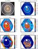 |
Fig. 1 a) SDSS stamp for NGC 2916 (CALIFA 277). As in other images throughout this paper, the circles mark R = 1 and 2 Half Light Radius (HLR). b) CALIFA image in the rest-frame 5635 ± 45 Å interval after applying the spatial mask. c) Map of the S/N at 5635 Å. d) S/N map after the Voronoi binning. e) Number of spaxels in each Voronoi zone. Note that no spatial binning (Nz = 1) was necessary throughout the inner ~1 HLR. f) Percentage of bad pixels in the 3800−6850 Å range. North is up and east is towards the left in all images. |
The following step (item v in our list) consists of applying a segmentation structure to the data, grouping spaxels into spatial zones. All spaxels belonging to the same zone are assigned a common integer ID label, unique for each zone. qbick stores the zone-to-xy tensor needed to map zones to pixels and vice-versa. In this paper we use spatial binning to increase the S/N for the spectral analysis. Other applications may prefer to group spaxels according to, say, morphology or emission-line oriented criteria. qbick admits an externally provided segmentation map to allow for such choices.
The zoning scheme adopted here is based on the Voronoi tesselation technique, as implemented by Cappellari & Copin (2003), but with modifications to account for correlated errors (Sect. 3.3). The code is fed with the signal and noise images in the 5635 ± 45 Å range discussed above. The target S/N is set to 20. In practice, most individual spaxels inside 1 HLR satisfy this condition. Figure 1d shows the S/N map of CALIFA 277 after the spatial binning. For this galaxy, the 3649 non-masked spaxels were grouped into 1638 zones, the overwhelming majority (1527) of which are not binned at all. As seen in the map of the number of spaxels per zone (Nz, Fig. 1e), spatial binning effectively starts at R ~ 1 HLR. Discounting the single spaxel zones, the median Nz is 10, but values up to 92 are reached in the outskirts.
Once the spatial binning map is defined, the flux, error, and flag spectra are computed
for each zone. This operation must account for the flagged pixels. The total flux in zone
z, which contains Nz
spaxels whose fluxes are Fλ,k, is given by
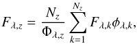 (1)where
φλ,k = 0 for flagged pixels
(bλ,k > 0) or 1
otherwise (bλ,k = 0), and
Φλ,z ≡ ∑ φλ,k
is the number of useful spaxels at wavelength λ in the zone. The zone
flux is thus Nz times the average flux over
all non-flagged pixels. When none of the Fλ,k
fluxes are flagged, this equation simply sums all the fluxes in the zone, whereas when
this is not the case, flagged entries are replaced by the average of non-flagged ones.
(1)where
φλ,k = 0 for flagged pixels
(bλ,k > 0) or 1
otherwise (bλ,k = 0), and
Φλ,z ≡ ∑ φλ,k
is the number of useful spaxels at wavelength λ in the zone. The zone
flux is thus Nz times the average flux over
all non-flagged pixels. When none of the Fλ,k
fluxes are flagged, this equation simply sums all the fluxes in the zone, whereas when
this is not the case, flagged entries are replaced by the average of non-flagged ones.
This scaling recipe is reasonable as long as the number of flagged pixels is not
comparable to Nz. For example, in a zone of
Nz = 10 spaxels, one would not like to take
the resulting Fλ,z seriously if eight of them
are flagged. We chose to flag away entries whenever fewer than half of the spaxels in a
zone have credible data at the given λ:
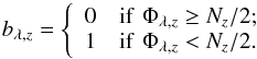 (2)For
our example galaxy, the fraction of flagged pixels in the 3800−6850 Å interval used in the
spectral synthesis analysis ranges from 5 to 8%, with a median of 6% (see Fig. 1f).
(2)For
our example galaxy, the fraction of flagged pixels in the 3800−6850 Å interval used in the
spectral synthesis analysis ranges from 5 to 8%, with a median of 6% (see Fig. 1f).
The computation of the error in Fλ,z follows
a recipe similar to Eq. (1), but adding in
quadrature: 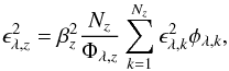 (3)where
βz accounts for correlated errors (see
below).
(3)where
βz accounts for correlated errors (see
below).
qbick also produces the total spatially integrated spectrum, following these same prescriptions. This is useful to compare the analysis of the whole to the sum of the analysis of the parts (which we do in Sect. 5.9).
Finally, all the spectra are resampled to 2 Å. The resulting zone spectra are stored in ASCII and/or FITS files, with flux, error, and flag columns necessary for a careful spectral analysis. All the quality control images produced in this process are packed in a single FITS file, along with the technical parameters adopted in the different steps (S/N clipping, segmentation map, etc.).
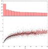 |
Fig. 2 Ratio of the measured over the idealized noise for Voronoi zones comprising Nz spaxels. The idealized noise is that derived under the assumption of uncorrelated errors, while the measured one is obtained from the detrended standard deviation of fluxes in a ± 45 Å range around 5635 Å. Gray dots represent βz values for 99267 spaxels from 109 galaxies. Circles show the median βz for each Nz, and the solid line shows Eq. (4). The top panel shows the histogram of Nz values (notice the logarithmic scale). |
3.3. Spatial binning and correlated errors
As mentioned, the datacubes have a spatial sampling of 1′′ × 1′′.
Because of the three-fold dithering pattern used in the observations, each spaxel has a
varying contribution from a number of fibers. Since one fiber can contribute to more than
one spaxel, the noise in a given spaxel is partially correlated with that of its
neighbors. This implies that when spectra from adjacent spaxels are added together the
noise in the resulting spectrum has to be calculated taking spatial covariances into
account. As an extreme example, consider Nz
completely correlated (i.e., ~identical) spaxels in a zone. Clearly, co-adding their
spectra would not result in the desired increase in the S/N as both signal and noise scale
linearly with Nz. Unless told otherwise,
however, the zoning algorithm assumes that the spaxels are independent and hence that the
noise in the zone is given by  ,
resulting in an improvement of the S/N of the co-added spectrum by
~
,
resulting in an improvement of the S/N of the co-added spectrum by
~ ,
whereas in fact it has not changed at all3.
,
whereas in fact it has not changed at all3.
An empirical correction was devised to account for the global behaviour of the spatial
correlation of the signal in CALIFA data. We proceed by first defining initial Voronoi
zones with the Cappellari & Copin (2003)
algorithm. Because it assumes uncorrelated input, the code presumes the zone error is
.
We then measure the “real” noise (ez) in the
resulting zone summed spectra from the (detrended) rms in the 5635 ± 45 Å range. The
ratio of these two numbers, which we call βz,
is represented versus the number of spaxels in each zone in Fig. 2. Small grey dots are βz
values for the individual zones, and circles represent the median value computed at each
Nz, while the shaded region represents the
16 to 84 percentiles. There are nearly 105 points in this plot, obtained from
244 196 spaxels in 109 galaxies (all those observed with the V500 and V1200 setups up to
May 2012). The top panel shows the histogram of
Nz.
The rise and flattening of the βz − Nz relation reflects the expected behavior. Zones with small Nz group adjacent and highly correlated spaxels, producing the initial rise of βz. As farther apart spaxels are aggregated, the errors become less correlated, leading to the flattening observed. The scatter in the relation is likely related to the way the Voronoi algorithm assemble spaxels. Also, the three-fold dithering pattern is not completely uniform, so the amount of correlation is not exactly the same across the face of the fiber bundle. Still, the βz(Nz) relation portrayed in Fig. 2 is tight enough to derive an excellent statistical correction.
The solid line represents the fit of the following function:  (4)where the fit was
carried out considering only the filled circles. We can now apply this correction directly
in the zoning code, replacing its idealized computation of the noise by
(4)where the fit was
carried out considering only the filled circles. We can now apply this correction directly
in the zoning code, replacing its idealized computation of the noise by
 (5)which accounts for the
effects of spatially correlated errors. This correction was applied λ by
λ (cf. Eq. (3)). An
independently derived correction very similar to Eq. (4) is presented in Husemann et al. (2013).
(5)which accounts for the
effects of spatially correlated errors. This correction was applied λ by
λ (cf. Eq. (3)). An
independently derived correction very similar to Eq. (4) is presented in Husemann et al. (2013).
While this scheme naturally leads to larger zones than those obtained under the (erroneous) hypothesis of independent spaxels, it ensures that the target S/N of 20 is actually achieved in all but the outermost zones (when the algorithm runs out of spaxels to bin). Typically, we obtain 1000 zones per galaxy.
4. STARLIGHT runs and PyCASSO
starlight is a spectral synthesis code which combines the spectra from a base in order to match an observed spectrum Oλ. The search for an optimal model Mλ and the coefficients of the population vector x associated with the N⋆ base elements also allows for reddening, a velocity off-set v⋆, and a stellar velocity dispersion σ⋆. The code was first introduced in Cid Fernandes et al. (2004) and substantially optimized by Cid Fernandes et al. (2005). The code, didactic introductions and a user manual are available at www.starlight.ufsc.br. We are using a new and yet to be documented version of starlight, but since most of the new features are not used in our analysis, the publicly available manual remains an accurate reference for the purposes of this paper.
The virtues and caveats of full spectral fits are discussed in a number of articles (e.g., Panter et al. 2003; Ocvirk et al. 2006; Cid Fernandes 2007; Tojeiro et al. 2007; McArthur et al. 2009; Sánchez-Blázquez et al. 2011). A general consensus in the field is that uncertainties in the results for individual objects average out for large statistical samples (Panter et al. 2007). With CALIFA, each galaxy is a statistical sample per se! Hence, even if the results for single spaxels (or zones) are not iron-clad, the overall trends should be robust (see Paper II for a detailed evaluation of the uncertainties in our starlight-based analysis of CALIFA data). It is also worth pointing out that despite the diversity of spectral synthesis methods, substantial changes in the results are more likely to come from revisions in the input data (as happened, for instance, with the recalibration of SDSS spectra between data releases 5 and 6) and from updates in the base models, the single most important ingredient in any spectral synthesis analysis.
The results reported in this paper rely on a spectral base of simple stellar populations (SSPs) comprising four metallicities, Z = 0.2, 0.4, 1, and 1,5 Z⊙, and 39 ages between t = 106 and 1.4 × 10¹⁰ yr. This base (dubbed “GM” in Paper II) combines the Granada models of González Delgado et al. (2005) for t < 63 Myr with those of Vazdekis et al. (2010; as updated by Falcón-Barroso et al. 2011) for larger ages. They are based on the Salpeter Initial Mass Function and the evolutionary tracks by Girardi et al. (2000), except for the youngest ages (≤3 Myr), which are based on Geneva tracks (Schaller et al. 1992; Schaerer et al. 1993a,b; Charbonnel et al. 1993). A comparison of results obtained with other bases and examples of the spectral fits are presented in Paper II.
The fits were carried out in the 3800−6850 Å interval. Reddening was modeled with the Cardelli et al. (1989) curve, with RV = 3.1. As in Cid Fernandes et al. (2005), the main emission lines as well as the NaI D doublet (because of its sensitivity to ISM absorption) were masked. All runs were performed in the IAA-GRID, a network of computers which allows us to process 105 spectra in less than a day.
As documented in the user manual, starlight outputs a large array of quantities. In broad terms, these can be categorized as:
-
1.
Input data: file names, configuration options, and other information provided either by the user explicitly or derived from the user-provided spectrum. Base-related data are also reported, including ages and metallicities of each component, the corresponding light-to-mass ratios (at the chosen normalization wavelength, λN), and a returned-mass correction factor.
-
2.
Fit results: figures of merit (χ2,
 ), kinematic
parameters (v⋆,
σ⋆), the V-band
extinction (AV), total stellar masses and
luminosities, and population vectors, expressed in terms of light (x) and
mass (μ) fractions.
), kinematic
parameters (v⋆,
σ⋆), the V-band
extinction (AV), total stellar masses and
luminosities, and population vectors, expressed in terms of light (x) and
mass (μ) fractions. -
3.
Spectral data: the input (Oλ), best-model fit (Mλ), and weight spectra (wλ, which equals
 ,
except for flagged, masked, and clipped pixels).
,
except for flagged, masked, and clipped pixels).
All these data are stored in a plain ASCII file, one for each fitted spectrum. The population vectors can be post-processed in a number of ways to obtain SFHs, compute the mass growth as a function of time, condense the results into first moments like the mean t and Z, etc. This scheme works fine for studies of independent objects, like SDSS galaxies or globular clusters.
IFS data, however, require a more structured level of organization, as it is cumbersome and inefficient to handle so many files separately. To handle datacubes we developed PyCASSO, which comprises three main parts:
-
1.
A writer module, which packs the output of all starlight fits of the individual zones of a same galaxy into a single (FITS or HDF5) file. This file also contains all information generated during the pre-processing steps (Sect. 3), as well as information propagated from the original datacube.
-
2.
A reader module, which reads this file and structures all the data in an easy to access and manipulate format.
-
3.
A post-processing module, which performs a series of common operations, such as mapping any property from zones to pixels, resampling and smoothing the population vectors, computing growth functions, and averaging in spatial, time or metallicity dimensions. All these functionalities are conveniently wrapped as python packages, easily imported into the user’s own analysis code.
5. Results
The Sb galaxy NGC 2916 (CALIFA 277) was chosen as a showcase. For the adopted distance of 56 Mpc, 1′′ (= 1 CALIFA spaxel) corresponds to 270 pc. With an r-band absolute magnitude of −21.17, u − r = 2.18 and g − r = 0.54 colors, and concentration index C = 2.16, NGC 2916 can be characterized as a blue-disk galaxy with an intermediate mass (~1011 M⊙). Rudnick et al. (2000) have shown that the galaxy presents some degree of lopsidedness, indicating a weak interaction (possibly with its irregular satellite 5′ away, Gutiérrez et al. 2002) or a minor merger. Moorthy & Holtzman (2006) have obtained long-slit spectra and measured emission lines and Lick indices along the position angle PA = −80°. They found that the nuclear spectrum is well within the AGN wing of the [Oiii]/Hβ vs. [Nii]/Hα diagram, in a location close to what is now accepted as borderline between Seyferts and LINERs (Kewley et al. 2006).
Our Voronoi binning of the CALIFA datacube produces N = 1638 zones. The corresponding N + 1 spectra (the + 1 corresponding to the spatially integrated spectrum) were fitted with starlight and the results feed into PyCASSO. The following subsections describe how we handled the data and the products of the analysis.
5.1. Fit quality assessment
As with 1D spectra, the quality of the spectral fits should be examined before proceeding to interpretation of the results. This subsection describes some standard methods to do this, the caveats involved and strategies to circumvent them.
Figure 3a shows the map of the fit quality indicator
 (6)where
Oλ and
Mλ are the observed and model spectra,
respectively, and the sum is carried over the
(6)where
Oλ and
Mλ are the observed and model spectra,
respectively, and the sum is carried over the  wavelengths actually used in the fit, i.e., discarding masked, flagged, and clipped
pixels4. For this galaxy
spans the
range between 1.0 and 5.6%, with a median value of 3.0%. It increases towards the outer
regions, where the S/N is smaller (Fig. 1c). The
wavelengths actually used in the fit, i.e., discarding masked, flagged, and clipped
pixels4. For this galaxy
spans the
range between 1.0 and 5.6%, with a median value of 3.0%. It increases towards the outer
regions, where the S/N is smaller (Fig. 1c). The
 map (Fig. 3b) shows the opposite behavior, since the errors also
increase outwards. Because of its non-explicit reliance on the (often hard to compute, if
not altogether unavailable) ϵλ spectrum, and
because of its easily grasped meaning, is a more useful
figure of merit to assess fit quality.
map (Fig. 3b) shows the opposite behavior, since the errors also
increase outwards. Because of its non-explicit reliance on the (often hard to compute, if
not altogether unavailable) ϵλ spectrum, and
because of its easily grasped meaning, is a more useful
figure of merit to assess fit quality.
Inspection of the highest spectra
often reveals non-masked emission lines or artifacts, like imperfect masking of foreground
sources, slightly misplaced bλ flags, or
Oλ values that should have been clipped by
starlight but were not because of large
ϵλ. We emphasize that such bugs are very
rare in CALIFA. The median for the
~105 zone spectra analyzed so far is just 4% (corresponding to an equivalent
S/N of 25), and in less than 2% of the cases exceeds 10%. This
high rate of success is mainly due to the carefully derived errors and flags in the
reduction pipeline and further refined in our pre-processing steps (Sect. 3).
One can use such maps to define spatial masks over which the spectral fits satisfy some
quality threshold. Experiments with the whole data set suggest that a reasonable
quality-control limit should be in the  to 10% range. Not surprisingly,
the large residuals tend to be located in the outer regions of the galaxies. Generally
speaking, results beyond 2−3 HLR should be interpreted with greater care. No
-based cut is
needed for our example galaxy. For the benefit of starlight users, it is
nevertheless worth making some further remarks on quality control.
to 10% range. Not surprisingly,
the large residuals tend to be located in the outer regions of the galaxies. Generally
speaking, results beyond 2−3 HLR should be interpreted with greater care. No
-based cut is
needed for our example galaxy. For the benefit of starlight users, it is
nevertheless worth making some further remarks on quality control.
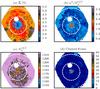 |
Fig. 3 Maps of spectral-fit quality indicators. a) Mean relative deviation
|
5.1.1. Subtleties and caveats on quality control
In full spectral fitting methods, seemingly trivial operations like imposing a fit quality threshold often hide subtleties that can easily go unnoticed, particularly when processing tons of data. The paragraphs below (focused on starlight but extensible to other codes) review some of these.
First, one should distinguish cases where is large because
of bad data from those where large residuals arise because of the user’s failure to
properly inform, through spectral masks
(mλ) or flags
(bλ), spectral regions that should be
ignored in the fit. For instance, one can have an excellent spectrum of an HII region
with several strong emission lines besides those included in a generic emission line
mask feed into starlight, causing an artificially large
. Large
velocity offsets can have a similar effect, as emission lines get shifted out of fixed
mλ windows. Similarly, sky residuals and
other artefacts missed out by the bλ flags
lead to large , even when
the overall spectrum is good. In short, not everything that fails a blind quality
control is actually bad.
The clipping options implemented in starlight help spot pixels that are too hard to fit and thus probably represent non-stellar or spurious features. Our fits use the “NSIGMA” clipping method and a conservative 4σ threshold, meaning that we only clip pixels when | Oλ − Mλ| > 4ϵλ. Figure 3c maps the number of clipped points in CALIFA 277. One sees a peak in the central pixels, where the S/N is so high that our 4σ clipping does not forgive even small Oλ − Mλ deviations (most often associated with problems with the base models rather than with the data). Elsewhere, very few pixels were clipped. The point to highlight here is that clipping only worked because we have a reliable ϵλ. Other clipping methods can be used when this is not the case, but in all cases the user should always carefully check the output, as it may easily happen that too many points are clipped.
Custom-made spectral masks also help. For instance, since Mateus et al. 2006), the starlight analysis of SDSS spectra employs individual masks constructed by searching for emission lines in the Oλ − Mλ residual spectrum obtained from a first fit, and taking into consideration the local noise level. Oλ is then refitted with this tailor-made mλ, circumventing some of the issues above. This refinement has not yet been implemented for CALIFA.
Errors, flags, and masks are, of course, secondary actors in any spectral synthesis analysis, but these general remarks illustrate that it is worthwhile to pay attention to them.
5.2. 2D maps: stellar light, mass, and extinction
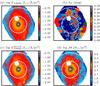 |
Fig. 4 a) Synthetic surface brightness at 5635 Å; b) stellar extinction map (AV); c) dereddened ℒλ5635 image; d) stellar mass surface density. |
One of the main products of spectral synthesis is to convert light to mass. Figure 4 illustrates the results for CALIFA 277. Its top-left panel shows the surface density of the luminosity at λN = 5635 Å, while the top-right panel show the derived extinction map. The dust corrected image and the mass surface density are also shown.
While the effects of the Voronoi binning are present in all panels, they are much more
salient in the AV map. This is because the
light and mass images were “dezonified” by scaling the value at each
xy spaxel by its fractional contribution to the total flux in a zone
(z). For instance, for the mass surface density (ℳ) this operation
reads 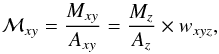 (7)where
Axy
(Az) denotes the area in a spaxel (zone),
and
(7)where
Axy
(Az) denotes the area in a spaxel (zone),
and  (8)with
Fxy as the mean flux in the 5635 ± 45 Å
region, the same used in the Voronoi zoning (Sect. 3). This operation was applied to luminosity and mass related quantities,
producing somewhat smoother images than obtained with
wxyz = 1. Intensive properties (like
AV, mean ages,
σ⋆), however, cannot be dezonified.
(8)with
Fxy as the mean flux in the 5635 ± 45 Å
region, the same used in the Voronoi zoning (Sect. 3). This operation was applied to luminosity and mass related quantities,
producing somewhat smoother images than obtained with
wxyz = 1. Intensive properties (like
AV, mean ages,
σ⋆), however, cannot be dezonified.
The stellar extinction map shows low values of AV (of order 0.1−0.2 mag), with slight enhancements in the nuclear region and the arms. Overall, however, there is relatively little variation across the face of the galaxy (see also Fig. 10). The light and mass images have a similar structure, both showing the bulge at R ≲ 0.5 HLR, and the disk beyond that. The spiral arms are less prominent in terms of mass than in light because of the higher L/M of stars in the arms.
The total stellar mass obtained from the sum of the zone masses is M = 6.5 × 10¹⁰ M⊙. This is the mass locked in stars nowadays. Counting also the mass returned by stars to the interstellar medium, M′ = 9.0 × 10¹⁰ M⊙ were involved in star formation. These values ignore the mass in the masked region around the foreground star northeast of the nucleus. PyCASSO can fill in such holes with values estimated from (circular or elliptical) radial profiles. For CALIFA 277, this correction increases the masses quote above by 4%.
5.3. 2D maps: kinematics
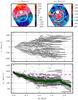 |
Fig. 5 Kinematical products of the spectral fitting. The σ⋆ values are not corrected for instrumental broadening, which dominates below 140 km s-1. The horizontal stripes in the position-velocity and σ⋆(R) panels correspond to Voronoi zones. |
Figure 5 shows the v⋆ and σ⋆ fields estimated by starlight, as well as a position-velocity diagram and a radially averaged σ⋆ profile. The v⋆ field indicates a projected rotation velocity of ~200 km s-1. The V500 resolution prevents the determination of σ⋆ values below ~150 km s-1, and the flat σ⋆(R) profile beyond ~0.7 HLR reflects this resolution limit (we have not corrected the values for the instrumental resolution in this plot). Only in the inner regions are the σ⋆ values reliable, reaching 200 km s-1 in the nucleus (equivalent to 140 km s-1 after correcting for instrumental broadening).
The kinematical information derived from our analysis will be superseded by studies based on the higher spectral resolution V1200 datacubes (Falcón-Barroso et al., in prep.). Eventually, one can envisage feeding the parameters derived from these more precise analyses back into the starlight fits (using its fixed-kinematics mode). In fact, this feedback may well turn out to improve our stellar population analysis, given the potential degeneracy between σ⋆ and Z (decreasing the former while increasing the latter has the same global effect of making metal lines deeper; Koleva et al. 2009; Sánchez-Blázquez et al. 2011).
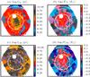 |
Fig. 6 Luminosity (top) and mass (bottom) weighted mean age (left) and metallicity (right) maps for CALIFA 277. |
5.4. 2D maps: mean ages and metallicities
The crudest way to quantify the SFH of a system is to compress the age and metallicity
distributions encoded in the population vectors to their first moments. For this purpose
we will use the following definitions: 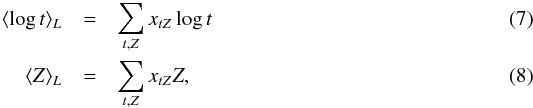 where
xtZ is the fraction of light at
λN due to the base population with age
t and metallicity Z. The mass-weighted versions of
these indicators, ⟨log t⟩M and
⟨Z⟩M, are obtained by replacing
xtZ by the mass fraction
μtZ.
where
xtZ is the fraction of light at
λN due to the base population with age
t and metallicity Z. The mass-weighted versions of
these indicators, ⟨log t⟩M and
⟨Z⟩M, are obtained by replacing
xtZ by the mass fraction
μtZ.
Figure 6 shows the light and mass-weighted mean (log) age and metallicity maps. The ⟨log t⟩L image shows a steady increase towards the center. Outside 1 HLR, traces of the spiral arms are noticeable as regions of lower age (as in the SDSS color image in Fig. 1a, the arms are brighter in the western half of the image). Because of the large weight of old populations, ⟨log t⟩M spans a smaller dynamical range than ⟨log t⟩L, hence producing lower contrast maps, but the outwardly decreasing age is still visible. Negative gradients are also clearly present in metallicity, with indications of flattening within the bulge region. As in other 2D maps, the small-scale fluctuations towards the edges are at least in part due to the lower S/N.
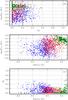 |
Fig. 7 Mean age versus mean metallicity versus extinction, coding zones by their distance to the nucleus. Green diamonds: R < 0.5 HLR. Red triangles: 0.5−1 HLR. Blue stars: 1−2 HLR. Black dots: > 2 HLR. |
The fact that t and Z grow in the same sense suggests that the results are not badly affected by the age-metallicity degeneracy. As shown by Sánchez-Blázquez et al. (2011), full spectral synthesis is much less sensitive to this than conventional index-based approaches. Figure 7 plots extinction versus mean age versus metallicity, the main properties involved in spectral synthesis. Points are color- and symbol-coded by their distance from the nucleus. One sees that the highest values of AV are found for old central (R < 0.5 HLR) and young outer (R > 1 HLR) populations and that AV bears no correlation with Z. The middle panel shows the positive t − Z relation inferred from the 2D maps. Within 0.5 HLR (green diamonds), however, t anticorrelates with Z, most likely due to the age-metallicity degeneracy. The mean Z values in this central region straddle 1 and 1.5 Z⊙, the two highest metallicities in our base.
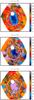 |
Fig. 8 Maps of the percentage contribution of young (t < 0.14 Gyr), intermediate age (0.14−1.4 Gyr), and old (>1.4 Gyr) stars to the observed light at 5635 Å. |
5.5. 2D maps: xY, xI, xO
Population synthesis studies in the past found that a useful way to summarize the SFH is to condense the age distribution encoded in the population vector into age ranges. This strategy comes from a time when the analysis was based on equivalent widths and colors (Bica 1988; Bica et al. 1994; Cid Fernandes et al. 2001, 2003), but it was also applied to full spectral fits (Gonzalez Delgado et al. 2004).
Figure 8 presents images of the light fraction due to young, intermediate and old populations (xY, xI, and xO), defined as those with t ≤ 0.14, 0.14 < t ≤ 1.4, and t > 1.4 Gyr, respectively. As usual, the choice of borderlines is somewhat subjective, constrained only by the underlying idea of grouping base elements covering relatively wide age ranges. For the base used in our starlight runs, the Y, I, and O bins contain 4 × 20, 4 × 10, and 4 × 9 SSPs, respectively (where the 4 × comes from the four metallicities).
The plots show that the spiral arms stand out more clearly in the xY map, specially in the western half of the galaxy, as also seen in the SDSS color composite (Fig. 1a). Very little of the light from R < 1 HLR comes from young stars. Intermediate age populations do contribute more, but the central ~0.5 HLR is completely dominated by old stars. Overall, however, despite the added informational content, these maps do not visibly add much to the ⟨log t⟩L image (Fig. 6).
5.6. 2D maps: Star formation rates and IFS-based variations over Scalo’s b parameter
The base used in our fits comprises instantaneous bursts (i.e., SSPs). Thus, despite the large number of ages considered, our SFHs are not continuous and hence not derivable. Nonetheless, there are ways of defining star formation rates (SFR).
The simplest way to estimate a SFR is to cumulate all the stellar mass formed since a
lookback time of tSF and perform a mass-over-time average:
 (11)where
 is the mass
(at xy and per unit area) of stars formed at lookback time
t 5. Equation (11) gives the mean SFR
surface density since t = tSF. One can tune
tSF to reach different depths in the past, but as
tSF increases this estimator becomes increasingly useless,
converging to the mass density divided by t∞ ≡ 14 Gyr (the
largest age in the base).
is the mass
(at xy and per unit area) of stars formed at lookback time
t 5. Equation (11) gives the mean SFR
surface density since t = tSF. One can tune
tSF to reach different depths in the past, but as
tSF increases this estimator becomes increasingly useless,
converging to the mass density divided by t∞ ≡ 14 Gyr (the
largest age in the base).
It is often more useful to consider SFRs in relation to some fiducial value instead of
absolute units. The classical example is Scalo’s birthrate parameter, b,
which measures the SFR in the recent past
(t < tSF) with
respect to its average over the whole lifetime of the system6. This is trivially obtained dividing  by its asymptotic value
 (12)The superscript
“loc” is to emphasize that the reference lifetime average SFR is that of the same spatial
location xy. One should recall that while young stars in a spaxel were
probably born there (or near it), old ones may have migrated from different regions. Thus,
despite the identical definitions, the physical meaning of
(12)The superscript
“loc” is to emphasize that the reference lifetime average SFR is that of the same spatial
location xy. One should recall that while young stars in a spaxel were
probably born there (or near it), old ones may have migrated from different regions. Thus,
despite the identical definitions, the physical meaning of
 is not
really the same as for galaxies as a whole.
is not
really the same as for galaxies as a whole.
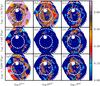 |
Fig. 9 Spatially resolved SFR surface density (Eq. (11)) on the last tSF = 14
(top), 142 (middle), and 1420
(bottom) Myr in units of different reference values. The
left panels compare |

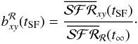
The IFS data allow for other definitions of b. For instance, one might
prefer to compare to the
 of the
galaxy as a whole, the bulge, the disk, or any general region. This variation measures the
“present” (t < tSF)
“here” (at xy) to the “past”
(t ≤ t∞) in a spatial region ℛ:
of the
galaxy as a whole, the bulge, the disk, or any general region. This variation measures the
“present” (t < tSF)
“here” (at xy) to the “past”
(t ≤ t∞) in a spatial region ℛ:
 (13)A formally
similar but conceptually different definition is obtained using for the reference value in
the denominator the SFR surface density within the same time-scale but
evaluated in a different region:
(13)A formally
similar but conceptually different definition is obtained using for the reference value in
the denominator the SFR surface density within the same time-scale but
evaluated in a different region: 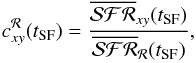 (14)i.e., to compare
not “now versus then” but “now here versus now there”. Together with Eqs. (12) and (13), this definition covers the different combinations of time and
space enabled by the application of fossil methods to IFS data.
(14)i.e., to compare
not “now versus then” but “now here versus now there”. Together with Eqs. (12) and (13), this definition covers the different combinations of time and
space enabled by the application of fossil methods to IFS data.
Figure 9 shows maps of
bloc (left panels), bℛ (middle
panels), and cℛ (right panels) for three values of
tSF: 14 (top), 142 (middle), and 1420 Myr (bottom). In all
panels the color scale is deliberately saturated to highlight regions where
 is
larger than the chosen reference value; the dynamical range of the images goes from 1 to 5
(0 to 0.7 in log) in the corresponding relative units.
is
larger than the chosen reference value; the dynamical range of the images goes from 1 to 5
(0 to 0.7 in log) in the corresponding relative units.
Panel a shows that spaxels that have formed stars over the past 14 Myr at a larger rate than their respective past average are all located in the outer regions. Nowhere within R ≲ 0.5 HLR does one find bloc(14 Myr) > 1. Considering the past 142 Myr (panel d), the inner “deficit” covers as much as 1.2 HLR. On the longest time scale considered (g), one again sees that the inner spaxels have been less active than their lifelong average.
Maps look considerably different in the middle column of panels, where the local
 is
normalized to the past average over the whole galaxy (Eq. (13)). The spiral arms of CALIFA 277 appear
better delineated in bgal(14 Myr) (panel b) than in any
bloc map. Interestingly, the
bgal map is practically featureless for
tSF = 142 Myr (e). This suggests that starformation is not
continuous over this time scale but instead happens in a bursty mode. Over the past 1.4
Gyr (h), one again sees traces of the arms but with a lower amplitude than in panel b,
which is qualitatively consistent with the cumulative effect of an intermittent sequence
of short-duration bursts. (Due to the logarithmic age resolution of fossil methods, such
short bursts can only be recognized as such at the very young ages sampled in panel b.)
is
normalized to the past average over the whole galaxy (Eq. (13)). The spiral arms of CALIFA 277 appear
better delineated in bgal(14 Myr) (panel b) than in any
bloc map. Interestingly, the
bgal map is practically featureless for
tSF = 142 Myr (e). This suggests that starformation is not
continuous over this time scale but instead happens in a bursty mode. Over the past 1.4
Gyr (h), one again sees traces of the arms but with a lower amplitude than in panel b,
which is qualitatively consistent with the cumulative effect of an intermittent sequence
of short-duration bursts. (Due to the logarithmic age resolution of fossil methods, such
short bursts can only be recognized as such at the very young ages sampled in panel b.)
The right column panels show our novel relative SFR index c (Eq. (14)), using the whole galaxy as reference region. Unlike Scalo’s b, this index does not compare present to past, but present to present elsewhere. Its 2D maps can be understood as “snapshots” of the SFR in the galaxy taken with an “exposure time” tSF. Keeping the “diaphragm” open for only the last 14 Myr (panel c) highlights the ongoing starformation in the galaxy. The spiral arms are clearly visible, and the structures are more focused than in the bgal(14 Myr) map (panel b). Integrating for 142 Myr (f), the inner parts of the arms fade, but their outer (R > 1 HLR) parts brighten up in terms of cgal. Over the past 142 Myr, these regions have formed more stars than anywhere else in the galaxy, even though a comparison with panel e shows that only parts of the cgal > 1 regions are forming stars at a rate per unit area larger than that of the galaxy as a whole through its entire life (i.e., bgal > 1). For tSF = 1.4 Gyr (panel i) the image becomes more blurred. Because of the long time scale, the cgal(1.4 Gyr) map is nearly indistinguishable from that obtained with bgal for the same tSF (panel h).
One thus sees that, despite some degree of redundancy (the numerator is always the same), these definitions offer different and complementary views of star formation in a galaxy.
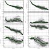 |
Fig. 10 Radial profiles of several properties. Grey points correspond to values in individual xy spaxels. The green circles and solid lines represent the average of the plotted quantity, while the error bars represent the dispersion in the R-bin. The dashed magenta horizontal line (only in the plots not involving surface densities) marks the value derived from the starlight analysis of the integrated spectrum, i.e., collapsing the xy dimensions of the datacube. The stars in the bottom panels mark the four metallicities in the base models. |
5.7. 1D spatial maps: radial profiles
The information contained in 2D maps like the ones shown above can sometimes be hard to absorb. Azimuthal averaging is a useful way to compress and help digest 2D data. PyCASSO provides both circular and elliptical xy-to-R conversion tensors. The examples below are based on a circular mapping.
For quantities like ℳ, one can think of two types of radial averaging. The first is to add up all the stellar mass in xy spaxels within a given R-bin and then divide by the bin area (counting only non-empty spaxels). The second is to average the surface density values for each spaxel directly. The same applies to, for instance, ⟨log t⟩L (Eq. (9)): one can either add up the value of product Ltxy × log t for all spaxels at a given R and then divide by the corresponding ∑ Lxy or else simply average the ⟨log t⟩L values for each spaxel in the R-bin. The first method, which we call area averaging, effectively collapses the galaxy to 1D, but this kind of averaging cannot be applied to quantities which do not involve light or mass, like AV and σ⋆. For the sake of uniformity, in this subsection we chose the second type of radial averaging (henceforth spaxel averaging), noting that the two methods almost always give nearly identical results.
Figure 10 shows several PyCASSO products as a function of R. The grey points represent values for individual spaxels. The solid line and green circles show the mean value of the plotted quantity among the spaxels in the same R bin, and the error bars map the corresponding dispersion. (As discussed in Paper II, actual error bars in radial profiles are much smaller due to the large number statistics.) Several of the features discussed while describing the 2D images are clearly seen in these plots. The ⟨log t⟩ and ⟨Z⟩ gradients, in particular, are cleanly depicted in these plots. As pointed out in Sect. 5.4, mean ages and metallicities increase ~simultaneously towards the nucleus, while AV does not change much. This indicates that the classical degeneracies in stellar population studies do not play a strong role in shaping the results, with the possible exception of the central regions. As in Fig. 5, horizontal stripes of gray points in panels c, e, f, g, and h of Fig. 10 correspond to spaxels in the same Voronoi zones. The stripes disappear in panels a, b, and d because these extensive quantities were “dezonified” (cf. Eq. (7)).
5.8. 1D temporal maps: evolutionary curves
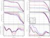 |
Fig. 11 Time evolution of light and mass representations of the SFH, as derived from the
starlight fits. The discrete
xtZxy and
|

The main power of fossil record methods is to open the time domain, allowing evolutionary studies. The caveat is that it does this with the typical logarithmic resolution inherent to stellar evolution, but several studies show that much can be learned about galaxy evolution despite this fundamental constraint. Because our 39 ages base is highly overdimensioned, some sort of SFH compression is necessary. As discussed by Asari et al. (2007), age resolutions between 0.5 and 1 dex are reasonable. We thus smooth the light and mass population vectors with a Gaussian of FWHM = 0.5 dex in log t.
Figure 11 plots a number of our synthesis products against age. To keep an at least partial representation of the spatial information, we plot evolutionary curves derived for different radial regions: the nucleus, defined as the central pixel (plotted in grey dashed lines), R ≤ 0.5 (dashed green), ≤1 (solid red), and >1 HLR (solid blue).
The top panels show the growth of luminosity (Fig. 11a) and mass (b)7. Among other things, this plot illustrates the difference between light and mass, in the sense that regions inside and outside R = 1 HLR do not have the same mass, despite having (by definition) the same light. While HLR = 4.8 kpc, the radius containing half of the mass is 3.4 kpc. This is a direct consequence of the stellar population gradients in this galaxy. González Delgado et al. (in prep.) investigate the relation between light- and mass-based radii for different types of galaxies.
It is also seen that both light and mass grow at different speeds for different
regions. This is better appreciated in panels c and d, where each growth curve
is plotted on a 0 to 1 scale, with 1 representing the present values (which tantamounts to
cumulating the equivalent xt and
 vectors for
each region). The nucleus reached 80% of its mass at t = 8.5 Gyr, while
the R > 1 HLR region did so later, at
t = 1.9 Gyr. As shown by Pérez et al. (2013), this inside-out ordering of the mass assembly history applies to
essentially all massive galaxies.
vectors for
each region). The nucleus reached 80% of its mass at t = 8.5 Gyr, while
the R > 1 HLR region did so later, at
t = 1.9 Gyr. As shown by Pérez et al. (2013), this inside-out ordering of the mass assembly history applies to
essentially all massive galaxies.
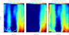 |
Fig. 12 R–t diagrams showing the radially averaged
distribution of light, mass, and SFR as a function distance from the nucleus and
age. Left: luminosity at λ = 5635 Å per unit area.
(ℒR,t). Middle: stellar mass formed
per unit area |


Figure 11e shows
 .
The SFR per unit area decreases from the nucleus outwards most of the time, but the trend
is reversed in the last ~500 Myr. Notice that, because of the smoothing,
is now a continuous function of time, so that this panel represents the
instantaneous SFR, as opposed to the mass-over-time definition in Eq.
(11). Figure 11f shows Scalos’s b parameter for each region, which
does use the running mean
.
The SFR per unit area decreases from the nucleus outwards most of the time, but the trend
is reversed in the last ~500 Myr. Notice that, because of the smoothing,
is now a continuous function of time, so that this panel represents the
instantaneous SFR, as opposed to the mass-over-time definition in Eq.
(11). Figure 11f shows Scalos’s b parameter for each region, which
does use the running mean  of Eq.
(11). This plot helps interpret Fig.
9, which opens up the radial regions into full 2D
maps but compress the time axis by stipulating fixed tSF time
scales.
of Eq.
(11). This plot helps interpret Fig.
9, which opens up the radial regions into full 2D
maps but compress the time axis by stipulating fixed tSF time
scales.
5.9. The whole versus the sum of the parts
One of the applications of CALIFA is to assess the effects of the lack of spatially resolved information on the derivation of physical properties and SFHs from integrated-spectra surveys. The horizontal dashed magenta lines in Fig. 10 illustrate this point. They represent the results obtained from the analysis of the spectrum of the datacube as a whole, that is, adding up all spaxels to emulate an integrated spectrum. Qualitatively, one expects that this should produce properties typical of the galaxy zones as a whole. This expectation is borne out in Fig. 10, where one sees that the extinction, mean ages, and metallicities marked by the dashed magenta line represent an overall average of the spatially resolved values. In this particular example, they all match quite well the values at 1 HLR. The stellar masses obtained from the whole and the sum of the parts are also in excellent agreement, differing by just 1%. Similarly, galaxy-wide luminosity and mass-weighted mean ages and metallicities computed in these two ways agree to within 0.05 dex.
But can one derive the SFH of a galaxy out of an integrated spectrum? Figure 11 says that, at least in CALIFA 277, the answer is yes. The dashed magenta and the black solid lines are very similar in all panels of this figure. As before, the former represents the results obtained from the analysis of the spatially compressed datacube, while the black curves are computed adding the starlight results for each spaxel. We are thus comparing the whole against the sum of the parts, and they match.
This may seem a trivial result, but it is not. Formally, one only expects this to happen if AV is the same at all positions, a condition which is approximately met in CALIFA 277. In objects where dust has strong spatial variations, the spectral fitting of the global spectrum with a single AV will inevitably operate compensations among the parameters, like increasing the age to compensate for an underestimated AV and viceversa. Also, the combined effects of population gradients and kinematics (e.g., disk population contributing more to the wings of absorption lines than the ones from the bulge) are hard to predict. Since we are presenting results for a single example galaxy, it remains to be seen how general this “coincidence” is.
5.10. Space × time diagrams: SFHs in 2D
One of the main challenges involved in the analysis of the multidimensional data built from the combination of the spatial dimensions with the t and Z dimensions opened by population synthesis is how to visualize the results. All examples shown so far project (or average over) two or more of these axes.
Figure 12 shows an attempt to visualize galaxy evolution as a function of both space and time. The trick is to compress xy into R and collapse the Z axis, producing a radially averaged SFH(R,t) map. The left panel shows the luminosity density ℒ at each radial position R and for each age t. As for the other panels in this figure, the original ℒtZyx array from which this map was derived was smoothed in log t, marginalized over Z, and collapsed into one spatial dimension. Unlike in Fig. 10, we now use the area-averaging method discussed in Sect. 5.7, but the results do not depend strongly on this choice.
The ℒR,t diagram shows that the light from old stars is
concentrated in the bulge, while the youngest stars shine at all R. Also,
t ≳ 1 Gyr stars are more smoothly distributed in age in the disk than
in the bulge, where they are concentrated in two populations, one at ~2.5 Gyr and the
other older than 10 Gyr. Figure 12b shows the formed
stellar mass surface density as a function of R and t.
As usual, due to the highly non-linear relation between light and mass in stars, the young
populations that show up so well in light practically disappear when seen in mass. Young
stars reappear in the right panel, which shows the evolution in time and space of the SFR
surface density. As in Fig. 11g, these are obtained
from the instantaneous SFR at each spaxel, computed as in Asari et al. (2007):
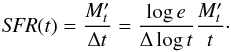 (15)The age sampling is
logarithmic (Δlog t = const.), so that the SFR is proportional to the
stellar mass formed at t divided by t. The
(15)The age sampling is
logarithmic (Δlog t = const.), so that the SFR is proportional to the
stellar mass formed at t divided by t. The
 and ℳ′R,t diagrams therefore carry the same
information; it is the t-1 factor that makes them look so
different.
and ℳ′R,t diagrams therefore carry the same
information; it is the t-1 factor that makes them look so
different.
When interpreting these or any other plot involving age, one should always keep in mind the logarithmic age resolution. For instance, taken at face value, the spatially integrated SFR of CALIFA 277 in the last few Myr is almost equal to its historical peak, ~2.5 Gyr ago (solid line in Fig. 12c). However, these two peaks span vastly different time intervals, roughly by a factor of Gyr/Myr = a thousand. The peak SFR around 2.5 Gyr ago, and indeed even well before that (at >10 Gyr, when most of the mass was formed), were surely higher than the one we are now seeing at a few Myr but cannot be resolved in time. No fossil record method will ever be able to distinguish bursts much shorter than their current age. These limitations are well known in the field, but it is fit to recall them to avoid misinterpretation of the results.
Notwithstanding such age resolution issues, Fig. 12 represents a novel way of looking at galaxies both in time and space. It shows clear evidence in favor of an inside-out growth scenario in which the outer regions assemble their mass at a slower pace and over a more extended period. This behavior is not unique to this galaxy. Pérez et al. (2012) find just the same in a study of the first 105 galaxies observed by CALIFA.
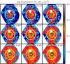 |
Fig. 13 “Pseudo snapshots” of the cumulative stellar mass surface density of CALIFA 277 at different ages: from log t [yr] = 10.15 to 8 (as labeled in each panel). |
5.11. Space vs. time “snapshots”
To go beyond the R–t diagrams of Fig. 12, one needs more dimensions than a sheet of paper can
accommodate. An alternative is shown in Fig. 13,
which shows t-slices through the cumulative
 cube.
Unlike the previous diagrams, which compressed the SFH in one way or another, these plots
reveal the full 2D nature of the mass assembly history of CALIFA 277.
cube.
Unlike the previous diagrams, which compressed the SFH in one way or another, these plots
reveal the full 2D nature of the mass assembly history of CALIFA 277.
Age sequences like those in Fig. 13 can be constructed for several, but not all, properties inferred though starlight or any other fossil method. One can, for instance, replace mass by intrinsic luminosity, SFR, or stellar metallicity in cumulative or differential form, but it is obviously impossible to reconstruct maps of AV, σ⋆, v⋆ as a function of t. It is also worth pointing out that the panels in Fig. 13 are not truly snapshots of a movie, that is, they are not pictures of the galaxy as it appeared at different look-back times. Instead, these are maps of where stars of a given age t are located nowadays.
Simulators should take notice of these simple facts. IFS data plus fossil methods provide a rich yet inevitably limited form of time travel. Illustrative and beautiful as they are, movies of stars and gas particles moving through time and space will never be directly compared to anything observational. In other words, simulations should be convolved through this “reality filter”. The observationally relevant predictions are the distribution of stellar ages and metallicities as a function of xy.
5.12. Emission line maps
Independent of the stellar population applications described throughout this paper, the starlight fits provide a residual spectrum Rλ = Oλ − Mλ that is, inasmuch as possible, free of stellar light. This is of great aid in the measurement of emission lines and hence in the derivation of a series of diagnostics of warm ISM properties, such as kinematics, nebular extinction, and chemical abundance. The complementarity of nebular and stellar analysis has been amply explored in studies of integrated spectra (e.g., Cid Fernandes et al. 2007; Asari et al. 2007; Pérez-Montero et al. 2010; García-Benito & Pérez-Montero 2012), and the addition of two spatial dimensions to this analysis holds great promise. Kehrig et al. (2012), for instance, combine starlight analysis and nebular emission to study the impact of post-AGB populations on the ionization of the ISM in early-type galaxies.
Figure 14 shows a Rλ,xy residuals cube with some of the main emission lines marked. The plot shows that emission lines are brighter towards the outside, in particular over the spiral arms, as could be guessed from the distribution of actively starforming regions traced by our SFH analysis (e.g., Fig. 9). Despite its active nucleus, the nuclear line fluxes are not particularly bright, implying a low-luminosity AGN.
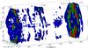 |
Fig. 14 Residual spectral cube in a 3D rendering. |
6. Summary
This paper described a complete “analysis pipeline”, which processes reduced IFS data through the starlight spectral synthesis code. Data for the spiral galaxy NGC 2916 (CALIFA 277) were used to illustrate the journey from (x,y,λ) datacubes to multidimensional maps of the synthesis products, focusing on the technical and methodological aspects. The three main steps in the analysis can be summarized as follows:
-
1.
Pre-processing: this step comprises (a) construction of a spatial mask; (b) adjustments in the flag and error spectra; (c) rest-framing and resampling; (d) spatial binning. The last three stages were coded in a generic python package (qbick), which can run in a fully automated fashion. Spatial binning was accomplished with a Voronoi tesselation scheme, which was tuned to produce zones with S/N ≥ 20 spectra. In practice, because of the good quality of the data, no binning was necessary within R ≲ 1 HLR. The issue of correlated errors in spatial binning was discussed and an empirical recipe to correct for it was presented. The output of these pre-processing steps are datacubes with fluxes, errors, and flags ready for a detailed λ-by-λ spectral analysis, as well as spatial masks, a zone map, and other ancillary products.
-
2.
starlight fits and organization of the synthesis results: Spectral fits for all spatial zones were performed using a base of SSP spectra from a combination of MILES and Granada models, spanning ages from 1 Myr to 14 Gyr and four metallicities between 0.2 and 1.5 solar. The results were packed in a coherent multilayered FITS (or HDF5) file with the Python Califa Starlight Synthesis Organizer (PyCASSO).
-
3.
Post-processing tools: PyCASSO includes a reader module and a series of analysis tools to perform operations like zone-to-pixel image reconstruction; mapping the spectral and stellar population properties derived by starlight into multidimensional time, metallicity, and spatial coordinates; averaging in spatial and temporal dimensions; manipulation of the stellar population arrays.
Some of the products of this whole analysis are standard in IFS work, like the kinematical field and emission line maps. The real novelty resides in the spatially resolved stellar population products recovered from the fossil record of galaxy evolution encoded in the datacubes. The 2D products range from maps of the stellar extinction and surface densities of stellar mass to more elaborate products like mean ages and metallicities, time-averaged star formation rates, and b-parameters. These quantities are all normally used in the analysis of integrated spectra, but their application to IFS data raises some conceptual issues related to the unavoidable fact that not all stars in a given spaxel were born there. On the other hand, one can use spatially resolved data to construct diagnostics unapplicable to integrated data, such as indices comparing the present and past SFR in different regions or comparing the “present here” with the “present elsewhere”. These IFS-based variations of the traditional b parameter were shown to be useful to highlight different aspects of the spatially resolved SFH.
1D profiles in temporal or radial coordinates helped interpret the results. In our example galaxy, these compressed views of the (t,Z,x,y) manifold reveal clear age and metallicity negative gradients, as well as spatially dependent mass growth speeds compatible with an inside-out formation scenario. Finally, radius-age diagrams and snapshot sequences were introduced as further means of visualization.
Clearly, the application of spectral synthesis methods to IFS datacubes offers new ways of studying galaxies and their evolution. Future communications will use the tools laid out in this paper to explore the astrophysical implications of the results for galaxies in the CALIFA survey.
Note that this is an apparently superfluous definition since we already have the noise spectrum. This “empirical” S/N is nevertheless useful, as explained in Sect. 3.3.
We note that Eq. (6) is nearly, but not
exactly, identical to what is called “adev” in starlight’s output, the difference
being the use of Mλ instead of
Oλ in the denominator. This avoids faulty
(but not flagged) Oλ entries with very low
flux affecting the statistics. This rarely occurs in CALIFA, and when it does the pixels
invariably have large errors and so are irrelevant for the fit. They can, however, affect
the value of .
The stellar mass in this equation differs from that in Eq. (7), Fig. 4, and the definitions of ⟨log t⟩M and ⟨Z⟩M. The latter are corrected by the mass returned to the medium by stars during their evolution (thus reflecting the mass currently in stars), while in the computation of SFRs this correction should not be applied. We distinguish the two types of stellar masses with the prime superscript (ℳ versus ℳ′).
A related index is the so-called specific SFR, which differs from b just by the t∞ factor in Eq. (12).
Acknowledgments
CALIFA is the first legacy survey performed at Calar Alto. The CALIFA collaboration would like to thank the IAA-CSIC and MPIA-MPG as major partners of the observatory and CAHA itself for the unique access to telescope time and support in manpower and infrastructure. We also thank the CAHA staff for their dedication to this project. R.C.F. thanks the hospitality of the IAA and the support of CAPES and CNPq. A.L.A. acknowledges support from INCT-A, Brazil. B.H. gratefully acknowledges the support by the DFG via grant Wi 1369/29-1. Support from the Spanish Ministerio de Economia y Competitividad through projects AYA2010-15081 (PI RGD), AYA2010-22111-C03-03 and AYA2010-10904E (SFS), AYA2010-21322-C03-02 (PSB) and the Ramón y Cajal Program (S.F.S., P.S.B. and J.F.B.) is warmly acknowledged. We also thank the Viabilidad, Diseño, Acceso y Mejora funding program ICTS-2009-10 for funding the data acquisition of this project.
References
- Asari, N. V., Cid Fernandes, R., Stasińska, G., et al. 2007, MNRAS, 381, 263 [NASA ADS] [CrossRef] [MathSciNet] [Google Scholar]
- Bell, E. F., Wolf, C., Meisenheimer, K., et al. 2004, ApJ, 608, 752 [NASA ADS] [CrossRef] [Google Scholar]
- Bertin, E., & Arnouts, S. 1996, A&AS, 117, 393 [NASA ADS] [CrossRef] [EDP Sciences] [Google Scholar]
- Bica, E. 1988, A&A, 195, 76 [NASA ADS] [Google Scholar]
- Bica, E., Alloin, D., & Schmitt, H. R. 1994, A&A, 283, 805 [NASA ADS] [Google Scholar]
- Blanc, G. A., Gebhardt, K., Heiderman, A., et al. 2010, in New Horizons in Astronomy: Frank N. Bash Symposium 2009, 432, 180 [Google Scholar]
- Bruzual, G., & Charlot, S. 2003, MNRAS, 344, 1000 [NASA ADS] [CrossRef] [Google Scholar]
- Cappellari, M., & Copin, Y. 2003, MNRAS, 342, 345 [NASA ADS] [CrossRef] [Google Scholar]
- Cardelli, J. A., Clayton, G. C., & Mathis, J. S. 1989, ApJ, 345, 245 [NASA ADS] [CrossRef] [Google Scholar]
- Charbonnel, C., Meynet, G., Maeder, A., Schaeller, G., & Schaerer, D. 1993, A&AS, 101, 415 [NASA ADS] [Google Scholar]
- Cid Fernandes, R. 2007, IAU Symp., 241, 461 [NASA ADS] [Google Scholar]
- Cid Fernandes, R., Mateus, A., Sodré, L., Stasińska, G., & Gomes, J. M. 2005, MNRAS, 358, 363 [NASA ADS] [CrossRef] [Google Scholar]
- Falcón-Barroso, J., Sánchez-Blázquez, P., Vazdekis, A., et al. 2011, A&A, 532, A95 [NASA ADS] [CrossRef] [EDP Sciences] [Google Scholar]
- Folkes, S., Ronen, S., Price, I., et al. 1999, MNRAS, 308, 459 [NASA ADS] [CrossRef] [Google Scholar]
- García-Benito, R., & Pérez-Montero, E. 2012, MNRAS, 423, 406 [NASA ADS] [CrossRef] [Google Scholar]
- González Delgado, R. M., Cerviño, M., Martins, L. P., Leitherer, C., & Hauschildt, P. H. 2005, MNRAS, 357, 945 [NASA ADS] [CrossRef] [Google Scholar]
- Gutiérrez, C. M., Azzaro, M., & Prada, F. 2002, ApJS, 141, 61 [NASA ADS] [CrossRef] [Google Scholar]
- Ilbert, O., Capak, P., Salvato, M., et al. 2009, ApJ, 690, 1236 [NASA ADS] [CrossRef] [Google Scholar]
- Kehrig, C., Monreal-Ibero, A., Papaderos, P., et al. 2012, A&A, 540, A11 [NASA ADS] [CrossRef] [EDP Sciences] [Google Scholar]
- Kelz, A., Verheijen, M. A. W., Roth, M. M., et al. 2006, PASP, 118, 129 [NASA ADS] [CrossRef] [Google Scholar]
- Koleva M., Prugniel P., & De Rijcke S. 2009, Astron. Nachr. 999, 1 [Google Scholar]
- Lilly, S. J., Le Fevre, O., Hammer, F., & Crampton, D. 1996, ApJ, 460, 1 [Google Scholar]
- MacArthur, L. A., González, J. J., & Courteau, S. 2009, MNRAS, 395, 28 [NASA ADS] [CrossRef] [Google Scholar]
- Madau, P., Ferguson, H. C., Dickinson, M. E., et al. 1996, MNRAS, 283, 1388 [NASA ADS] [CrossRef] [Google Scholar]
- Moles, M., Benítez, N., Aguerri, J. A. L., et al. 2008, AJ, 136, 1325 [Google Scholar]
- Moorthy, B. K., & Holtzman, J. A. 2006, MNRAS, 371, 538 [Google Scholar]
- Ocvirk, P., Pichon, C., Lançon, A., & Thiébaut, E. 2006, MNRAS, 365, 46 [NASA ADS] [CrossRef] [Google Scholar]
- Panter, B., Heavens, A. F., & Jimenez, R. 2003, MNRAS, 343, 1145 [NASA ADS] [CrossRef] [MathSciNet] [Google Scholar]
- Panter, B., Jimenez, R., Heavens, A. F., & Charlot, S. 2007, MNRAS, 378, 1550 [NASA ADS] [CrossRef] [Google Scholar]
- Pérez, E., Cid Fernandes, R., González Delgado, R. M., et al. 2013, ApJ, 764, L1 [NASA ADS] [CrossRef] [Google Scholar]
- Pérez-González, P. G., Rieke, G. H., Villar, V., et al. 2008, ApJ, 675, 234 [NASA ADS] [CrossRef] [Google Scholar]
- Pérez-Montero, E., García-Benito, R., Hägele, G. F., & Díaz, Á. I. 2010, MNRAS, 404, 2037 [NASA ADS] [Google Scholar]
- Roth, M. M., Kelz, A., Fechner, T., et al. 2005, PASP, 117, 62 [Google Scholar]
- Rudnick, G., Rix, H.-W., Kennicutt, R. C., Jr. 2000, ApJ, 538, 569 [NASA ADS] [CrossRef] [Google Scholar]
- Sánchez, S. F., Kennicutt, R. C., Gil de Paz, A., et al. 2012, A&A, 538, A8 [NASA ADS] [CrossRef] [EDP Sciences] [Google Scholar]
- Sánchez-Blázquez, P., Ocvirk, P., Gibson, B. K., Pérez, I., & Peletier, R. F. 2011, MNRAS, 415, 709 [NASA ADS] [CrossRef] [Google Scholar]
- Schaerer, D., Charbonnel, C., Meynet, G., Maeder, A., & Schaller, G. 1993a, A&A, 102, 339 [Google Scholar]
- Schaerer, D., Meynet, G., Maeder, A., & Schaller, G. 1993b, A&AS, 98, 523 [NASA ADS] [Google Scholar]
- Schaller, G., Schaerer, D., Meynet, G., & Maeder, A. 1992, A&AS, 96, 269 [Google Scholar]
- Tojeiro, R., Heavens, A. F., Jimenez, R., & Panter, B. 2007, MNRAS, 381, 1252 [NASA ADS] [CrossRef] [Google Scholar]
- Vazdekis, A., Sńchez-Blázquez, P., Falcón-Barroso, J., et al. 2010, MNRAS, 404, 1639 [NASA ADS] [Google Scholar]
- Verheijen, M. A. W., Bershady, M. A., Andersen, D. R., et al. 2004, Astron. Nachr., 325, 151 [NASA ADS] [CrossRef] [Google Scholar]
- York, D. G., Adelman, J., Anderson, J. E., et al. 2000, AJ, 120, 1579 [Google Scholar]
- Walcher, J., Groves, B., Budavári, T., & Dale, D. 2011, Ap&SS, 331, 1 [NASA ADS] [CrossRef] [Google Scholar]
All Figures
|
Fig. 1 a) SDSS stamp for NGC 2916 (CALIFA 277). As in other images throughout this paper, the circles mark R = 1 and 2 Half Light Radius (HLR). b) CALIFA image in the rest-frame 5635 ± 45 Å interval after applying the spatial mask. c) Map of the S/N at 5635 Å. d) S/N map after the Voronoi binning. e) Number of spaxels in each Voronoi zone. Note that no spatial binning (Nz = 1) was necessary throughout the inner ~1 HLR. f) Percentage of bad pixels in the 3800−6850 Å range. North is up and east is towards the left in all images. |
| In the text | |
|
Fig. 2 Ratio of the measured over the idealized noise for Voronoi zones comprising Nz spaxels. The idealized noise is that derived under the assumption of uncorrelated errors, while the measured one is obtained from the detrended standard deviation of fluxes in a ± 45 Å range around 5635 Å. Gray dots represent βz values for 99267 spaxels from 109 galaxies. Circles show the median βz for each Nz, and the solid line shows Eq. (4). The top panel shows the histogram of Nz values (notice the logarithmic scale). |
| In the text | |
|
Fig. 3 Maps of spectral-fit quality indicators. a) Mean relative deviation
|
| In the text | |
|
Fig. 4 a) Synthetic surface brightness at 5635 Å; b) stellar extinction map (AV); c) dereddened ℒλ5635 image; d) stellar mass surface density. |
| In the text | |
|
Fig. 5 Kinematical products of the spectral fitting. The σ⋆ values are not corrected for instrumental broadening, which dominates below 140 km s-1. The horizontal stripes in the position-velocity and σ⋆(R) panels correspond to Voronoi zones. |
| In the text | |
|
Fig. 6 Luminosity (top) and mass (bottom) weighted mean age (left) and metallicity (right) maps for CALIFA 277. |
| In the text | |
|
Fig. 7 Mean age versus mean metallicity versus extinction, coding zones by their distance to the nucleus. Green diamonds: R < 0.5 HLR. Red triangles: 0.5−1 HLR. Blue stars: 1−2 HLR. Black dots: > 2 HLR. |
| In the text | |
|
Fig. 8 Maps of the percentage contribution of young (t < 0.14 Gyr), intermediate age (0.14−1.4 Gyr), and old (>1.4 Gyr) stars to the observed light at 5635 Å. |
| In the text | |
|
Fig. 9 Spatially resolved SFR surface density (Eq. (11)) on the last tSF = 14
(top), 142 (middle), and 1420
(bottom) Myr in units of different reference values. The
left panels compare |
| In the text | |
|
Fig. 10 Radial profiles of several properties. Grey points correspond to values in individual xy spaxels. The green circles and solid lines represent the average of the plotted quantity, while the error bars represent the dispersion in the R-bin. The dashed magenta horizontal line (only in the plots not involving surface densities) marks the value derived from the starlight analysis of the integrated spectrum, i.e., collapsing the xy dimensions of the datacube. The stars in the bottom panels mark the four metallicities in the base models. |
| In the text | |
|
Fig. 11 Time evolution of light and mass representations of the SFH, as derived from the
starlight fits. The discrete
xtZxy and
|
| In the text | |
|
Fig. 12 R–t diagrams showing the radially averaged
distribution of light, mass, and SFR as a function distance from the nucleus and
age. Left: luminosity at λ = 5635 Å per unit area.
(ℒR,t). Middle: stellar mass formed
per unit area |
| In the text | |
|
Fig. 13 “Pseudo snapshots” of the cumulative stellar mass surface density of CALIFA 277 at different ages: from log t [yr] = 10.15 to 8 (as labeled in each panel). |
| In the text | |
|
Fig. 14 Residual spectral cube in a 3D rendering. |
| In the text | |
Current usage metrics show cumulative count of Article Views (full-text article views including HTML views, PDF and ePub downloads, according to the available data) and Abstracts Views on Vision4Press platform.
Data correspond to usage on the plateform after 2015. The current usage metrics is available 48-96 hours after online publication and is updated daily on week days.
Initial download of the metrics may take a while.