| Issue |
A&A
Volume 556, August 2013
|
|
|---|---|---|
| Article Number | A42 | |
| Number of page(s) | 11 | |
| Section | Extragalactic astronomy | |
| DOI | https://doi.org/10.1051/0004-6361/201321455 | |
| Published online | 23 July 2013 | |
The occulting galaxy pair UGC 3995
Dust properties from HST and CALIFA data⋆
1 European Space Agency Research Fellow (ESTEC), Keplerlaan 1, 2200 AG Noordwijk, The Netherlands
e-mail: This email address is being protected from spambots. You need JavaScript enabled to view it.
2 Department of Physics and Astronomy, University of Alabama, Box 870324, Tuscaloosa, AL 35487, USA
Received: 12 March 2013
Accepted: 23 May 2013
Abstract
UGC 3995 is an interacting and occulting galaxy pair. UGC 3995B is a foreground face-on spiral and UGC 3995A a bright background spiral with an AGN. We present analysis of the dust in the disc of UGC 3995B based on archival Hubble Space Telescope (HST) WFPC2 and PPAK IFU data from the CALIFA survey’s first data release.
From the HST F606W image, we construct an extinction map by modeling the isophotes of the background galaxy UGC 3995A and the resulting transmission through UGC 3995B. This extinction map of UGC 3995B shows several distinct spiral extinction features. The radial distribution of AV values declines slowly with peaks corresponding to the spiral structures. The distribution of AV values in the HST extinction map peaks near AV = 0.3–0.4. Beyond this point, the distribution of AV values drops like an exponential: N(AV) = N0 × e(−AV/0.5). The 0.5 value is higher than typical for a spiral galaxy. The outer arms may be tidally distended; the extinction in the corresponding interarm regions is small to an unusually small radius.
To analyze the PPAK IFU data, we take the ratio of a fibre spectrum in the overlap region and the corresponding background fiber spectrum to construct an extinction curve. We fit the Cardelli, Clayton and Mathis (CCM) curve to the extinction curve of each fiber element in the overlap region. A map of the extinction constructed from PPEX IFU data-cubes shows the same spiral structure of the HST extinction map but the some differences in the distribution of the normalization of the CCM fits (AV). The inferred extinction slopes (RV) maps do not display any structure and a range of values partly due to the sampling effects of the disc by fibers, sometimes due to bad fits, and possibly partly due to some reprocessing of dust grains in the interacting disc.
We compare these findings to our other analysis of an occulting pair with HST and IFU data. In both cases the canonical RV = 3.1 is not recovered even though there is enough signal in the extinction curve. We attribute this to mixing opaque and more transparent sections of the disc in each resolution element (~3′′ or 0.9 kpc). To illustrate the difficulty of imposing a RV = 3.1 law over a section of a spiral disc, we average all spectra and show how a fully gray extinction curve is recovered.
Key words: techniques: spectroscopic / dust, extinction / galaxies: ISM / galaxies: dwarf / galaxies: individual: UGC 3995 / galaxies: structure
Appendix A is available in electronic form at http://www.aanda.org
© ESO, 2013
1. Introduction
The distribution of interstellar dust in spiral galaxies is still a dominant unknown in many areas of extra-galactic astrophysics, e.g., models of the spectral energy distribution (SED) of spiral galaxies (e.g., Popescu et al. 2000; Popescu & Tuffs 2005; Pierini et al. 2004; Baes et al. 2003, 2010; Bianchi et al. 2000; Bianchi 2007, 2008; Driver et al. 2008; Jonsson et al. 2010; Wild et al. 2011; Holwerda et al. 2012a; Verstappen et al., in prep.; Holwerda et al., in prep.) or distance measurements (e.g., SNIa, Jha et al. 2007; Holwerda 2008).
Dust is typically studied by either its characteristic far-infrared and sub-millimeter emission or its absorption of starlight in the ultraviolet and optical bands. The former approach needs sufficient data to solve for both dust surface density and temperature, requiring a solid detection in multiple bands to break this degeneracy. The latter, in contrast, works even for arbitrarily cold grains, but requires a background light source of known brightness.
Our knowledge of the geometry of dust in external galaxies has seen great improvements with the Herschel Space Observatory. These have mapped the temperature gradient in the dusty interstellar medium (ISM; Bendo et al. 2010; Smith et al. 2010; Engelbracht et al. 2010; Pohlen et al. 2010; Foyle et al. 2012), notably in the spiral arms (Bendo et al. 2010) and bulge (Engelbracht et al. 2010) and the power spectrum of the ISM, gas and dust (Combes et al. 2012). In the case of dwarf galaxies, Spitzer and results are restricted to a few individual galaxies (e.g., Hinz et al. 2006, 2012; Hermelo et al. 2013), the Herschel Virgo Cluster Survey (Grossi et al. 2010), or results of stacked observations (Popescu et al. 2002; de Looze et al. 2010; Bourne et al. 2012). However, the smallest scales can still only be probed in some of the most nearby galaxies, e.g., Andromeda, the Magellanic Clouds or the Milky Way itself. Thus, there is a niche for observations in the optical or ultra-violet to estimate dust geometry in spiral discs independently from sub-mm observations.
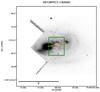 |
Fig. 1 Inverse grayscale plot of the HST/WFPC2 F606W image with the overlap aperture (green box). UGC 3995B is the foreground spiral on the right, UGC 3995A is the bright background spiral on the left. The nucleus of UGC 3995A was the target of GO-5479 with the Planetary Camera part of the WFPC2. The orange line shows over which the radial profile in Fig. 3 was taken. |
To map dust extinction on the smallest scales, one needs a smooth and known background source of light. In the case of a spiral galaxy overlapping a more distant galaxy, the more distant galaxy provides the known background (Fig. 1). Estimating dust extinction and mass from differential photometry in occulting pairs of galaxies was first proposed by White & Keel (1992). Their technique was then applied to all known pairs using ground-based optical images (Andredakis & van der Kruit 1992; Berlind et al. 1997; Domingue et al. 1999; White et al. 2000), spectroscopy (Domingue et al. 2000), and later space-based Hubble Space Telescope (HST) images (Keel & White 2001a,b; Elmegreen et al. 2001; Holwerda et al. 2009, H09 hereafter). The general results of this technique have been confirmed with the number of distant galaxies seen through spiral discs with HST (González et al. 1998, 2003; Holwerda 2005b,a; Holwerda et al. 2005a,b,c,e,d, 2007a,c, 2012b). More recently, more pairs were found in the SDSS spectroscopic catalog (86 pairs in Holwerda et al. 2007b), and in the Galaxy Zoo project (1993 pairs in Keel et al. 2013).
One of these, UGC 3995, an already known interacting pair (Keel 1986, 1985; Chatzichristou 1997; Chatzichristou et al. 1998; Marziani et al. 1999; Dultzin-Hacyan et al. 1999), was observed with the PPAK IFU as part of the first data-release of the Calar Alto Legacy Integral Field Area Survey (CALIFA, Sánchez et al. 2012) as well as with HST as early as 1994. The wealth of data on this particular pair offers the opportunity to study both small-scales dust extinction features from the Hubble data and the mean and variance of the extinction curve in the foreground spiral from the CALIFA data-cube. The fact that this is a known interacting pair – similar to the pair studied in Elmegreen et al. (2001) – offers the opportunity to compare the characteristics of the dust disc of a late-type foreground spiral to those of the other superb examples of an overlapping pair presented in Holwerda et al. (2009) and Holwerda et al. (2013), which we suspect is not interacting.
In this paper we aim to map the dust in UGC 3995B1 through the HST and CALIFA data and the extinction curves inferred from the CALIFA cubes. The paper is organised as follows: Sect. 2 briefly describes the data-products used, Sect. 3 describes the observational effects in the occulting galaxy technique, Sect. 4 details the analysis and results on both data-sets, Sect. 5 is the discussion of the results and Sect. 6 lists our conclusions and outlines for future work. We adopt a distance 67 Mpc, from the mean redshift and H0 = 71 km s-1 Mpc-1.
2. Data
We use two public data sets for this paper: archival Hubble images, and the two final data-cubes from the first CALIFA data release (DR1, November 2012 Husemann et al. 2013).
2.1. HST/WFPC2
A single WFPC2 F606W snapshot image, exposed for 500 s, of this pair was obtained by the HST in cycle 4 (GO-5479, P.I. M. Malkan, as described by Malkan et al. (1998) to image the substructure in and around the active center of the background galaxy with the Planetary Camera). Therefore, the PC chip is centered on the nucleus of the background galaxy, UGC 3995A (Fig. 1). Data were obtained from the Hubble Legacy Archive2 and cosmic rays cleaned interactively before analysis.
2.2. The CALIFA survey
The Calar Alto Legacy Integral Field Area Survey (CALIFA, Sánchez et al. 2012) is observing a sample of some 600 galaxies in the local Universe using 250 observing nights with the PMAS/PPAK integral field spectrophotometer, mounted on the Calar Alto 3.5 m telescope. The PPAK instrument offers a combination of a wide field-of-view (2.25 arcmin2) with a high filling factor in one single pointing (65%), good spatial sampling (1′′) and wavelength coverage spanning the optical spectrum. The spectra cover the range 3700–7000 Å in two overlapping setups, one in the red (3745–7300 Å) at a spectral resolution of R ≃ 850 (the V500 cubes) and one in the blue (3400–4750 Å) at R ≃ 1650 (V1200 cubes), where the spectral resolutions quoted are those in the overlapping wavelength range (λ ~ 4500 Å). The targets were selected from the photometric catalog of the Sloan Digital Sky Survey limited in apparent isophotal diameter to fit the PPAK field-of-view. A second selection criterion is a redshift range within 0.005 < z < 0.03, which ensures that all galaxies can be observed with the same grating settings. This approach suits our purpose well as it samples the overlap region to physical scales which could be small enough to resolve the dust structures needed to measure the extinction law (Keel & White 2001a; Holwerda et al. 2009). However, the small velocity difference (Δv ~ 50 km s-1) between UGC 3995 A and B almost certainly means that the spectral cross-correlation technique pioneered in Domingue et al. (2000) would require sub-Ångstrom spectral sampling. CALIFA observations started in summer 2010 and the first data release was in November 2012. Here we use the data cubes publicly available for UGC 3995 from DR1 (Husemann et al. 2013). More occulting galaxy pairs are slated to be observed by CALIFA3.
2.2.1. Fibre-transmission and sky-subtraction
The CALIFA data-reduction is described in detail by Sánchez et al. (2012). We focus on the relative fibre spectral transmission and the sky-subtraction because these are the most relevant for our fibre-to-fibre comparison to obtain extinction curves.
The relative transmission of the fibres is calibrated with a lamp spectrum. The accuracy of the relative transmission is better than a few percent in most of the covered fibres. The initial absolute spectrophotometric calibration was relatively poor (24% on average nights, and poorer in non-photometric condition) but the final product is accurate to ~8% after a re-calibration using the SDSS imaging of these galaxies (see Sect. 5.7 in Sánchez et al. 2012). The relative transmission affects the measured slope of the extinction curve (RV) and the absolute calibration the normalization of this curve (AV).
The subtraction of the night-sky spectrum from the data is an issue in many IFU observations of nearby galaxies, mostly due to the relatively small field-of-view and the resulting lack of a pure night-sky spectrum, uncontaminated by source flux. We note the VIMOS/IFU observations in Holwerda et al. (2013) were an exception, because that pair was small enough on the sky. By design, the apparent size of the galaxies in CALIFA fit within the FoV of the central bundle of the PPAK IFU. The PPAK IFU has 36 dedicated sky fibers, positioned such that they are free from any source contamination. With these clean sky-fibres, subtraction is straightforward and not a main source of uncertainty: the sky-subtraction has an accuracy of 1–5%.
2.2.2. Spatial resolution
The PPAK has a relatively coarse sampling of the field-of-view. To mitigate this, a well-understood three-pointing dithering strategy was adopted for the CALIFA survey (Sánchez et al. 2012). Night-specific measurements of the seeing conditions are presented for DR1 observations in Husemann et al. (2013): typical seeing was 0 9 and thus is not the limiting factor in the spatial resolution of the CALIFA data cube. The image reconstruction algorithm of the dithered observations resulted in a typical spatial resolution of 3′′ FWHM (similar to the fibre diameter of 27), as verified with bright stars in the FOV. We adopt a fiber size of 1′′, and resolution 3′′, verified by an examination of the star in Fig. 6 in both cubes. Improvements in the spatial sampling are expected in future data-releases of CALIFA.
3. Observational effects
There are three observational effects to consider in extinction measurement using an occulting pair of galaxies: intrinsic asymmetry of either galaxy, light scattered into the line-of-sight and the effects of physical sampling of the foreground ISM. We want to point them out to the reader and briefly review them.
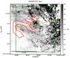 |
Fig. 2 Extinction map, corresponding approximately to the overlap region marked in Fig. 1, in which we identified the inter-arm regions of UGC 3995B by eye (red polygon), surrounding complex A and B in Fig. 2. The orange line shows where the transmission curve from the center of UGC 3995A to the center of UGC 3995B, shown in Fig. 3, was taken. |
3.1. Symmetry of both galaxies
The central assumption in our analysis of the HST and IFU data is that both galaxies are rotationally symmetric. This assumption of symmetry must especially hold for the background galaxy. For this reason, we would prefer an elliptical galaxy as a background. However, in this case it is a grand-design spiral. For this reason, observations in the red are preferred as spirals appear more regular without much structure from star-formation which often breaks symmetry on small scales.
In principle, the dark dust structure visible in the HST image (Figs. 1 and 2) and the attenuation evident in the IFU data could be part of the background galaxy. That would uncharacteristically break symmetry for the background galaxy, and secondly, the general morphology of the dusty structures strongly suggests that they belong to the foreground disc (orientation, implied winding angle) and not the background galaxy. The dust lies on the extrapolated spiral arm pattern of the foreground galaxy, not the background galaxy’s. However, the deviations from symmetry due to either local star-formation or extinction in the background galaxy are likely the dominant uncertainty in the extinction measurement.
3.2. Scattering
Because the galaxies are not point sources but extended objects, the relation between attenuation and wavelength may include effects of background galaxy light scattered into the line-of-sight by dust clouds in the foreground disc. This effect is treated in detail in the appendix of White et al. (2000). There are two extended sources of scattered light, the foreground and background galaxy.
The foreground galaxy contribution is removed in the HST analysis through subtraction. The contribution of light from the foreground galaxy scattered within the foreground itself is removed by the symmetry in our analysis: the subtraction of the foreground flux in Eq. (1) leaves no foreground scattered light. This leaves the background galaxy as the main source of scattered light in our measurements. The effect of scattering is greatest in regions of modest optical depth (τ ~ 1) and brightest background source (close to the background galaxy’s nucleus). Any opaque regions are self-absorbing and this effect does not matter.
White et al. (2000) examine the contribution of scattered light into a line-of-sight as a function of angular and radial separation of the two galaxies. If the galaxies are sufficiently far apart, the scattering angle becomes negligible. They express the scattering percentage as a function of the ratio between radial extent and separation of both discs. Given the small velocity and distance separation between UGC 3995A and UGC 3995B (Δ ~ 50 km s-1 velocity separation4), one would expect an effect of several percent of observed flux in the overlap. The main effects would be to lower the contrast between opaque and transparent regions in the HST extinction map and, because scattering affects blue light more than red, a grayer observed extinction curve.
3.3. Sampling
In H09, we already noted the effect of spatial sampling on the observed extinction law. By mixing opaque and transparent regions in the same resolution element, the effectively observed extinction curve becomes much less wavelength dependent, i.e., a “gray” extinction law (RV ≪ 3.1, see Calzetti et al. 1994). This has little effect on the HST extinction map as it possesses exquisite spatial resolution and no colour information. However, this can be an important observational effect in the CALIFA results. We return to this in the discussion of the results below.
4. Analysis
Analysis of the HST and CALIFA data is discussed separately with a third section comparing the results.
4.1. HST data analysis
The analysis of the HST/WFPC2 image (Fig. 1) extends the work by Marziani et al. (1999) with a more detailed procedure. We use elliptical isophote fits to the unobscured part of UGC 3995A to model its light distribution, supplementing the HST image with the SDSS r data in the gaps around the PC CCD, and use symmetry of UGC 3995B to correct for the contribution of foreground light. We found this approach the most reliable in H09 for the application of this method to HST data. The geometry of the UGC 3995 pair is especially favorable, in that the outer arms of UGC 3995B are projected in front of the bright, strongly bulge-dominated parts of UGC 3995A. Departures from the symmetry assumptions will be manifested differently for the two galaxies, largely following the spiral patterns of the respective galaxies. For the radial extinction profile, averaging azimuthally (or along the arm pitch angle) has the effect of marginalizing over the nuisance parameter of location along the background arm.
The transmission T, which is the fraction of incident light reaching us through the foreground galaxy, is well behaved to errors from either galaxy model, i.e., it depends on either linearly, and we use this quantity to map extinction. As in White & Keel (1992) and H09, if B and F are the intensities of background and foreground galaxies at each point estimated from symmetry or modeling, T may be estimated from the observed intensity I following:  (1)T is related to the extinction of the dust in the foreground disc as:
 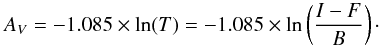 (2)Figure 2 shows the extinction (AV) map, based on the WFPC2 field. There is clear noise at the edges of the FOV as the background galaxy contribution is the lowest. Several foreground stars remain as artifacts. However, in the aperture (green box), there is sufficient signal-to-noise ratio (S/N) for a meaningful extinction measure (AV). Several spiral arms are evident in extinction (regions A and B in Fig. 2, also visible in Fig. 1) with a myriad of substructure in each arm.
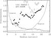 |
Fig. 3 Radial plot of the transmission T, which is the fraction of incident light reaching us through the foreground galaxy. Solid points are the averaged radial profile of transmission, with error bars at each radius from the scatter in measurements (error of the mean in each case). Open symbols show inter-arm regions as identified in the transmission map (Fig. 2), in regions of high expected S/N. Solid lines are the intensity of light from foreground (UGC 3995B) and background (UGC 3995A) galaxies along the line between both nuclei (the orange line in Fig. 1), to the same but arbitrary scale. |
Figure 3 shows the averaged radial profile of transmission from the HST image, with error bars at each radius from the scatter in measurements (error of the mean in each case); open symbols show inter-arm regions as identified in the transmission map, in regions of high expected S/N. This is an unusually complete profile in radius from the overlap technique, comparable to that of NGC 3314A shown by Keel & White (2001b). The curves in Fig. 3 show the intensity of light from foreground and background galaxies along the line between nuclei (orange line in 2), as evaluated from our modeling of symmetric foreground and ellipse-fit background. This provides a guide to how much scatter is introduced by structure in the foreground galaxy, which is important where it is much brighter than the background. These intensity curves of the foreground and background galaxy are to the same (arbitrary) scale.
The dust lanes in the outer arms are systematically offset to greater radius with respect to the stellar light associated with the spiral arm (Fig. 3); dust leads stellar spiral structure. The reliable identification of individual extinction features becomes progressively less certain toward the center of UGC 3995B, since the background light is weaker and the amplitude of contaminating foreground features becomes larger. Conversely, the dust in several of the outer arms is particularly well and reliably mapped, e.g., complexes A and B in Fig. 2. In Fig. 3, we note a fairly sharp edge to the occurrence of these dust lanes at 21′′ (6.8 kpc), about 1.6 disc scale lengths based on fitting the radial profile of the non-backlit part of the galaxy (orange line in Fig. 2).
In Fig. 2 the inter-arm regions can be clearly distinguished in the outer disc of UGC 3558B, partly by their lower extinction. Their transmission are the open points in Fig. 3. Inter-arm regions are mostly transparent but block up to 20% of the light of the background galaxy. Some inter-arm measurements show transmission greater than unity, the result of asymmetry in the background galaxy’s light distribution.
The arm geometry seen in absorption agrees with the visual impression that UGC 3995B is viewed essentially face-on, so we make no additional corrections for projection effects in estimating optical depths. At least on the eastern (backlit) side of the disc, the dust arms lie systematically outside the ridge line of stellar arms.
Figure 4 shows the histogram of the overlap aperture in Fig. 2. The distribution peaks at AV ~ 0.25, which is unusual for the outer disc of a spiral galaxy. In the pair we analyzed in H09 and Holwerda et al. (2013), the distribution gradually declines from a maximum at AV = 0. We suspect that this other pair is not interacting (the respective redshifts in that case imply a separation of ~4 Mpc, still within the velocity range of bound pairs, so their interaction status remains ambiguous). The redshift separation between UGC 3995A and B is only ~50 km s-1, so they are certainly tidally interacting. A recent or ongoing tidal interaction might be responsible for the redistribution into denser clouds through compression, shocks and triggered collapse. The offset of the peak from AV = 0 and the high value of the exponential decline in Fig. 4 could be related to the very transparent interarm regions noted above, if the outer arms are at least partly tidally shaped; tidal interaction removed diffuse inter-arm dust into dense concentrations in the arms.
We fit an exponential to the decline of the distribution in Fig. 4 beyond AV = 0.5. We find an exponential drop of 0.5, i.e., the number of pixels with value AV can be well described as N(AV) = N0 × e(− AV/0.5). This value is higher than we found in H09 and it is not typical of the exponential distribution used as a prior, for example, in SN Ia lightcurve fits (typically the drop-off is 0.3).
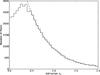 |
Fig. 4 Distribution of AV values in the green aperture in Figs. 1 or 2. The dashed line is an exponential drop fit to the values beyond AV = 0.5. Above this value, the distribution of pixels with is well described by N = N0 × e(− AV/0.5) with N0 = 6799 pixels. |
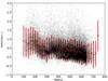 |
Fig. 5 Projected distance from the center of UGC 3995B in arcseconds versus the extinction (AV). Gray points are individual pixel values in the aperture in Fig. 2, the red points and error bars are the median and rms of these values. |
Figure 5 shows the radial distribution of all the extinction measurements in the overlap aperture (green rectangle in Fig. 2) and their median. The extinction gradually decreases with distance from the center of the foreground galaxy UGC 3995B. Two bumps in the mean value point to the spiral structures visible in Figs. 1 and 2.
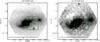 |
Fig. 6 Summed PPAK data-cubes from the CALIFA, the V500 (left) and V1200 (right). |
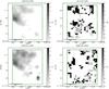 |
Fig. 7 Maps of the normalization (AV) and slope (RV) of the CCM fit to the fiber extinction curves (τ = −1.086 × ln (OL/BG)) from the V500 and the V1200 cubes. The normalization follows the extinction map in Fig. 2 but the slope, RV is unrelated to the extinction in the HST image. |
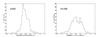 |
Fig. 8 Distribution of normalization (AV) values in the aperture region (Fig. 6) for the CCM fits to the extinction curves in the fibers in the V500 (left) and V1200 (right) cube. Because the wavelength range is different for each cube, a different normalization can be expected. |
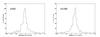 |
Fig. 9 Distribution of the slope (RV) values in the aperture region (Fig. 6) for the CCM fits to the extinction curves in the fibers in the V500 (left) and V1200 (right) cube. |
4.2. CALIFA data
The CALIFA data cubes were analyzed fiber-by-fiber, assuming again that the light contribution from the foreground galaxy is negligible compared to the bright background galaxy (valid mostly in the outer disc). The HST results show where the approximation of no foreground contamination is applicable: where the outer disc of UGC 3995B projected against inner bulge of UGC 3995A. However, we are somewhat forced into this approach, as the corresponding aperture is not available in the PPAK field-of-view (Fig. 6). We limit the analysis to the same aperture as used for the HST data (green box in Figs. 1) for ease of comparison.
To obtain the extinction curve in each fiber in the aperture, we find the corresponding fiber in the background galaxy by rotating the position 180° around the central position of the UGC 3995B (RA = 116.03393, Dec = 29.247411). The extinction curve, A(λ), follows from the ratio of the overlap spectrum, OL(λ), in the aperture and the background galaxy spectrum, BG(λ), in the corresponding fiber: 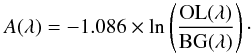 (3)An example of the OL and BG fiber spectra and the resulting extinction curve is shown in Fig. 10. The extinction curve in many individual fibers is of sufficient S/N to fit the extinction law parameterization of Cardelli et al. (1989) to each:
 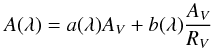 (4)where a(λ) and b(λ) are the polynomials determined by Cardelli et al. (1989) and AV and RV are the normalization and slope of the fit. We compute the polynomials for the wavelength range and subsequently perform a linear fit to A(λ) with AV and RV as free parameters with numpy.polyfit in the python environment. We fit both CALIFA cubes over most of their respective wavelength ranges: we fit over the sub-range 5200–7300 Å for the V500 low-resolution cube and 4000–4700 Å for the high-resolution V1200 cube, to avoid edge-effects in the extinction slopes.
Figure 7 shows the overlap aperture and the values of the AV and RV for each fiber fit in both the low-resolution cube (V500) and high-resolution cube (V1200). The two normalization (AV) maps agree qualitatively very well, although there are some patches of higher extinction in the Northern structure in the high-resolution and bluer cube (V1200). The higher values of the extinction slope normalization are, in part, due to a fit to a wavelength range blueward of the reference Johnson V band; the value is extrapolated for comparison, from the spectral range observed to Johnson V (5500 Å). The lower-resolution V500 cube actually includes the Johnson V. We noted in H09 that the foreground dust disc appears patchier in the bluer wavebands as well. The result is robust with smoothing in the spectral direction (Figs. A.1 and A.3).
In contrast, the RV maps are almost random and the results from both cubes compare poorly with each other. The random pattern of RV values persists in the fits of fiber spectra after these were spectrally smoothed to boost S/N (Figs. A.2 and A.4), that is, these spectral data are not sufficient in sampling and S/N to trace the R parameter.
The distributions of AV and RV derived for both cubes are shown in Figs. 8 and 9. The normalization behaves approximately as one can expect. The mean AV is zero, implying little to no sign of an extinction law in the overlap region.
Figure 11 shows the mean extinction curves taken over the aperture for the V500 and V1200 cubes. In this case, we do not average in the spectral direction but spatially over the whole overlap aperture. The resulting curve is extremely flat as it combines known high and low extinction areas. It serves to illustrate how, if one takes a large aperture over a spiral disc, the extinction law always becomes essentially flat (RV = 1).
4.3. Comparing HST and PPAK results
The normalization maps follow the extinction map in Fig. 2 reasonably well: there are two spiral structures visible in the North and East of the aperture (complexes A and C in Fig. 2) but certainly not all the (spiral arm) structure visible in Fig. 2 can be identified in Fig. 7. The agreement between the results from both CALIFA cubes is good as well.
The distributions of AV values in Fig. 8 for both CALIFA cubes show a different range of values than Fig. 4; there are more negative values as well as a more gradual decrease. The V500 values peak at AV = −0.2, the V1200 cube’s distribution is closer to Fig. 4; values extend closer to AV = 2 and there is a peak at AV = 0.5 but there is another peak at AV = 0. corresponding to the part of the aperture in Fig. 6 not covered by UGC 3995B.
There are three differences between the two data-sets: spatial resolution, S/N in each resolution element, and the spectral range. The spatial resolution of the HST data is significantly better than that of the CALIFA cube, even if the S/N is substantially lower as it is only broad-band information. Spectral coverage of the V500 curve includes the Johnson V filter, while the high-resolution V1200 cube does not.
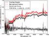 |
Fig. 10 Good example of two fiber spectra from the V500 cube: one fiber spectrum from the overlap region (OL, black solid line), its counterpart in a corresponding background fiber (BG, red solid line) and the resulting extinction curve (dashed line) and CCM fit to that extinction curve (dotted line). |
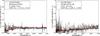 |
Fig. 11 Mean extinction curve of the overlap region (green box in Fig. 6) in the V500 (left) and V1200 (right) cubes. This is to illustrate the effect of spatially smoothing an extinction signal over a spiral disc: little or any extinction is detected and no slope in the extinction |
5. Discussion
UGC 3995 is only the second galaxy pair for which serendipitously, both HST and IFU data are available. However, unlike the pair analyzed in Holwerda et al. (2013), we are certain this one is interacting strongly. The UGC 3995 pair has several advantages though: it is a factor four closer (z = 0.015812 to z = 0.06) than our other pair and the foreground galaxy is close to face-on. The spatial sampling of the foreground disc is therefore much better in UGC 3995: ~ 30 pc for the HST (PSF =  ) data. However, the CALIFA spatial resolution is ~ 3′′ (Husemann et al. 2013), which translates to ~ 0.9 kpc.
The physical scale of the CALIFA cubes is still at least a factor ten above the maximum we determined for recovering a Milky-Way extinction law from Hubble color-imaging of a few galaxy pairs (~100 pc. Keel & White 2001a, H09)5. If the slope of the extinction law is determined over both highly opaque and mostly transparent sections, the extinction law effectively becomes gray (low values of RV, see also Natta & Panagia 1984; Keel & White 2001a; Holwerda et al. 2009; Grosbøl & Dottori 2012). Thus, the lower range in extinction curve slopes visible in Fig. 7 can be explained by the mixing of transparent and opaque regions. In their comparison between galaxy-wide SEDs in Wild et al. (2011) find extinction laws very similar to the Milky Way one. The measured dust reddening in this case is dominated by the optically thin parts of the galaxy discs; the reddening of the observed light is accurately retrieved but the total light absorption is not (as opaque regions are effectively not included).
High values of RV may point to recently formed or reprocessed dust or just poor fits. If the high RV values are indeed real, they may point to cases where large grains have yet to coalesce or have been disintegrated by shocks or a strong ultraviolet radiation field (e.g., through shocks or recently formed stars).
In a comparison with the other galaxy pair we have both IFU (VIMOS) and HST data for (Holwerda et al. 2009) and Holwerda et al. (2013), two things stand out: the distribution of AV values and the range of RV values fit in the fibers. The spatial sampling by the VIMOS data is ~ 0.9 kpc (both seeing and sampling are ~07) so we expect a equally grayer relation: we find in a similar overlap RV values between 1 and 3 with sensible fits in most fibers. Here we find a much greater range of RV values. In part this maybe because the symmetry argument does not hold completely for UGC 3445B anymore as it is in interacting. Asymmetry would compound any problematic fits to the extinction curves. Overlapping discs will have to be sampled more finely in the future if we are to recover the extinction curve’s slope.
The distribution of extinction values in the HST data is in our view telling: it peaks not at the typical AV = 0 but AV = 0.3, even though a similar fraction of the foreground disc is overlapping and covered by HST and IFU observations. The redistribution is either the result of a strong asymmetry in UGC 3995A, the background galaxy, or the result of an actual redistribution of dust in the disc of UGC 3995B. The latter might take the form of moving dust from low to higher column densities or removing a large fraction of the diffuse dust disc (destruction of grains). Arguing in favor of the redistribution is the more extended distribution beyond AV = 0.4 and the effectively empty inter-arm regions.
6. Conclusions
-
1.
UGC 3995B shows several spiral extinctionfeatures (Fig. 2).
-
2.
The geometry of this system allows construction of an unusually complete transmission map from HST data at 6000 Å, and from this radially-averaged distributions of transmission for the whole disc and for interarm regions (Fig. 3).
-
3.
The distribution of AV values in the HST extinction map peaks near AV = 0.3 − 0.4, unlike the distribution observed in other galaxies (Fig. 4).
-
4.
Beyond this point, the distribution of AV values drops like an exponential: N(AV) = N0 × e(− AV/0.5). The 0.5 value is higher than typical for a spiral galaxy (Fig. 4).
-
5.
The radial distribution of AV values declines slowly (Fig. 5).
-
6.
A map of the extinction constructed from PPEX IFU data-cubes shows the same spiral structure of the HST extinction map (Figs. 2, 7, A.1 and A.3).
-
7.
The inferred extinction slope (RV) maps do not display any structure and a range of values partly due to the sampling of the disc by fibers and possibly partly due to the reprocessing of dust grains in the interacting disc (Figs. 7–9).
Future applications of IFU observations could shed more light on the composition of late-type discs, provided the spatial sampling is sufficient. Ongoing efforts to equip existing telescopes with improved IFUs (e.g., the WEAVE instrument on WHT or the MUSE on VLT6) will have the spatial resolution, field-of-view, and spectral range to facilitate detailed mapping of the effective extinction law, and thus dust grain distribution, in occulting galaxy pairs.
Online material
Appendix A: Smoothing the CALIFA cubes
The following figures show the effect of smoothing the high (V1200) and low-resolution (V500) CALIFA cubes in the spectral direction on the resulting CCM extinction curve fits, both the normalization (AV) and slope (RV).
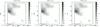 |
Fig. A.1 Extinction in the overlap region (green box in Fig. 6) in the V500 cube. The spectra were not smoothed (left panel), and smoothed by 10 and 14 Å (middle and right panels respectively) before a CCM extinction curve was fit to it. These panels show the normalization (AV) of the fit. |
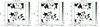 |
Fig. A.2 Extinction law in the overlap region (green box in Fig. 6) in the V500 cube. The spectra were not smoothed (left panel), and smoothed by 10 and 14 Å (middle and right panels respectively) before a CCM extinction curve was fit to it. These panels show the slope (RV) of the fit. |
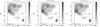 |
Fig. A.3 Extinction in the overlap region (green box in Fig. 6) in the first part of the V1200 cube. The spectra were not smoothed (left panel), and smoothed by 3.5 and 4.9 Å (middle and right panels respectively) before a CCM extinction curve was fit to it. These panels show the normalization (AV) of the fit. |
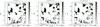 |
Fig. A.4 Extinction curve in the overlap region (green box in Fig. 6) in the first part of the V1200 cube. The spectra were not smoothed (left panel), and smoothed by 3.5 and 4.9 Å (middle and right panels respectively) before a CCM extinction curve was fit to it. These panels show the slope (RV) of the fit. |
The galaxies were already identified as UGC 3995 A and B for the background and foreground galaxy. Obviously, UGC 3995B for the foreground galaxy is not optimal terminology in our paper here but we retain it throughout for consistency.
An interacting system could have a Δv = 300 km s-1 and yet be spatially coincident. Unfortunately, more accurate distances for both galaxies are not available.
Unfortunately, no multifilter HST imaging is available for UGC 3995, or a similar extinction law measurement could have been made.
Acknowledgments
The authors would like to thank the anonymous referee for a thoughtful and comprehensive rapport. The lead author thanks the European Space Agency for the support of the Research Fellowship program. This research has made use of the NASA/IPAC Extragalactic Database (NED) which is operated by the Jet Propulsion Laboratory, California Institute of Technology, under contract with the National Aeronautics and Space Administration. This research has made use of NASA’s Astrophysics Data System. Plots were made using the matplotlib environment in Python (Hunter 2007). This study makes uses of the data provided by the Calar Alto Legacy Integral Field Area (CALIFA) survey (http://califa.caha.es/). Based on observations collected at the Centro Astronómico Hispano Alemán (CAHA) at Calar Alto, operated jointly by the Max-Planck-Institut für Astronomie and the Instituto de Astrofisica de Andalucia (CSIC).
References
- Andredakis, Y. C., & van der Kruit, P. C. 1992, A&A, 265, 396 [NASA ADS] [Google Scholar]
- Baes, M., Davies, J. I., Dejonghe, H., et al. 2003, MNRAS, 343, 1081 [NASA ADS] [CrossRef] [Google Scholar]
- Baes, M., Fritz, J., Gadotti, D. A., et al. 2010, A&A, 518, L39 [NASA ADS] [CrossRef] [EDP Sciences] [Google Scholar]
- Bendo, G. J., Wilson, C. D., Warren, B. E., et al. 2010, MNRAS, 402, 1409 [NASA ADS] [CrossRef] [Google Scholar]
- Berlind, A. A., Quillen, A. C., Pogge, R. W., & Sellgren, K. 1997, AJ, 114, 107 [NASA ADS] [CrossRef] [Google Scholar]
- Bianchi, S. 2007, A&A, 471, 765 [NASA ADS] [CrossRef] [EDP Sciences] [Google Scholar]
- Bianchi, S. 2008, A&A, 490, 461 [NASA ADS] [CrossRef] [EDP Sciences] [Google Scholar]
- Bianchi, S., Davies, J. I., & Alton, P. B. 2000, A&A, 359, 65 [NASA ADS] [Google Scholar]
- Bourne, N., Maddox, S. J., Dunne, L., et al. 2012, MNRAS, 421, 3027 [NASA ADS] [CrossRef] [Google Scholar]
- Calzetti, D., Kinney, A. L., & Storchi-Bergmann, T. 1994, ApJ, 429, 582 [NASA ADS] [CrossRef] [Google Scholar]
- Cardelli, J. A., Clayton, G. C., & Mathis, J. S. 1989, ApJ, 345, 245 [NASA ADS] [CrossRef] [Google Scholar]
- Chatzichristou, E. T. 1997, in Joint European and National Astronomical Meeting, eds. J. D. Hadjidemetrioy, & J. H. Seiradakis [Google Scholar]
- Chatzichristou, E. T., Vanderriest, C., & Lehnert, M. 1998, A&A, 330, 841 [NASA ADS] [Google Scholar]
- Combes, F., Boquien, M., Kramer, C., et al. 2012, A&A, 539, A67 [NASA ADS] [CrossRef] [EDP Sciences] [Google Scholar]
- de Looze, I., Baes, M., Zibetti, S., et al. 2010, A&A, 518, L54 [NASA ADS] [CrossRef] [EDP Sciences] [Google Scholar]
- Domingue, D. L., Keel, W. C., Ryder, S. D., & White, III, R. E. 1999, AJ, 118, 1542 [NASA ADS] [CrossRef] [Google Scholar]
- Domingue, D. L., Keel, W. C., & White, III, R. E. 2000, ApJ, 545, 171 [NASA ADS] [CrossRef] [Google Scholar]
- Driver, S. P., Popescu, C. C., Tuffs, R. J., et al. 2008, ApJ, 678, L101 [NASA ADS] [CrossRef] [Google Scholar]
- Dultzin-Hacyan, D., Marziani, P., & D’Onofrio, M. 1999, in Galaxy Interactions at Low and High Redshift, eds. J. E. Barnes, & D. B. Sanders, IAU Symp., 186, 352 [Google Scholar]
- Elmegreen, D. M., Kaufman, M., Elmegreen, B. G., et al. 2001, AJ, 121, 182 [NASA ADS] [CrossRef] [Google Scholar]
- Engelbracht, C. W., Hunt, L. K., Skibba, R. A., et al. 2010, A&A, 518, L56 [NASA ADS] [CrossRef] [EDP Sciences] [Google Scholar]
- Foyle, K., Wilson, C. D., Mentuch, E., et al. 2012, MNRAS, 421, 2917 [NASA ADS] [CrossRef] [Google Scholar]
- González, R. A., Allen, R. J., Dirsch, B., et al. 1998, ApJ, 506, 152 [NASA ADS] [CrossRef] [Google Scholar]
- González, R. A., Loinard, L., Allen, R. J., & Muller, S. 2003, AJ, 125, 1182 [NASA ADS] [CrossRef] [Google Scholar]
- Grosbøl, P., & Dottori, H. 2012, A&A, 542, A39 [NASA ADS] [CrossRef] [EDP Sciences] [Google Scholar]
- Grossi, M., Hunt, L. K., Madden, S., et al. 2010, A&A, 518, L52 [NASA ADS] [CrossRef] [EDP Sciences] [Google Scholar]
- Hermelo, I., Lisenfeld, U., Relaño, M., et al. 2013, A&A, 549, A70 [NASA ADS] [CrossRef] [EDP Sciences] [Google Scholar]
- Hinz, J. L., Misselt, K., Rieke, M. J., et al. 2006, ApJ, 651, 874 [NASA ADS] [CrossRef] [Google Scholar]
- Hinz, J. L., Engelbracht, C. W., Skibba, R., et al. 2012, ApJ, 756, 75 [NASA ADS] [CrossRef] [Google Scholar]
- Holwerda, B. W. 2005a, in HST Proposal, 6982 [Google Scholar]
- Holwerda, B. W. 2005b, Ph.D. Thesis, Proefschrift, Rijksuniversiteit Groningen [Google Scholar]
- Holwerda, B. W. 2008, MNRAS, 386, 475 [NASA ADS] [CrossRef] [Google Scholar]
- Holwerda, B. W., González, R. A., Allen, R. J., & van der Kruit, P. C. 2005a, AJ, 129, 1381 [NASA ADS] [CrossRef] [Google Scholar]
- Holwerda, B. W., González, R. A., Allen, R. J., & van der Kruit, P. C. 2005b, AJ, 129, 1396 [NASA ADS] [CrossRef] [Google Scholar]
- Holwerda, B. W., González, R. A., Allen, R. J., & van der Kruit, P. C. 2005c, A&A, 444, 101 [NASA ADS] [CrossRef] [EDP Sciences] [Google Scholar]
- Holwerda, B. W., González, R. A., Allen, R. J., & van der Kruit, P. C. 2005d, A&A, 444, 319 [NASA ADS] [CrossRef] [EDP Sciences] [Google Scholar]
- Holwerda, B. W., González, R. A., van der Kruit, P. C., & Allen, R. J. 2005e, A&A, 444, 109 [NASA ADS] [CrossRef] [EDP Sciences] [Google Scholar]
- Holwerda, B. W., Draine, B., Gordon, K. D., et al. 2007a, AJ, 134, 2226 [NASA ADS] [CrossRef] [Google Scholar]
- Holwerda, B. W., Keel, W. C., & Bolton, A. 2007b, AJ, 134, 2385 [NASA ADS] [CrossRef] [Google Scholar]
- Holwerda, B. W., Meyer, M., Regan, M., et al. 2007c, AJ, 134, 1655 [NASA ADS] [CrossRef] [Google Scholar]
- Holwerda, B. W., Keel, W. C., Williams, B., Dalcanton, J. J., & de Jong, R. S. 2009, AJ, 137, 3000 [NASA ADS] [CrossRef] [Google Scholar]
- Holwerda, B. W., Bianchi, S., Böker, T., et al. 2012a, A&A, 541, L5 [NASA ADS] [CrossRef] [EDP Sciences] [Google Scholar]
- Holwerda, B. W., Pirzkal, N., & Heiner, J. S. 2012b, MNRAS, 427, 3159 [NASA ADS] [CrossRef] [Google Scholar]
- Holwerda, B. W., Boker, T., Dalcanton, J. J., Keel, W. C., & de Jong, R. S. 2013 [arXiv:1304.3615] [Google Scholar]
- Hunter, J. D. 2007, Computing In Science & Engineering, 9, 90 [Google Scholar]
- Husemann, B., Jahnke, K., Sánchez, S. F., et al. 2013, A&A, 549, A87 [NASA ADS] [CrossRef] [EDP Sciences] [Google Scholar]
- Jha, S., Riess, A. G., & Kirshner, R. P. 2007, ApJ, 659, 122 [NASA ADS] [CrossRef] [Google Scholar]
- Jonsson, P., Groves, B. A., & Cox, T. J. 2010, MNRAS, 403, 17 [NASA ADS] [CrossRef] [Google Scholar]
- Keel, W. C. 1985, AJ, 90, 2207 [NASA ADS] [CrossRef] [Google Scholar]
- Keel, W. C. 1986, in Structure and Evolution of Active Galactic Nuclei, eds. G. Giuricin, M. Mezzetti, M. Ramella, & F. Mardirossian, Astrophys. Space Sci. Lib., 121, 579 [Google Scholar]
- Keel, W. C., & White, III, R. E. 2001a, AJ, 121, 1442 [NASA ADS] [CrossRef] [Google Scholar]
- Keel, W. C., & White, III, R. E. 2001b, AJ, 122, 1369 [NASA ADS] [CrossRef] [Google Scholar]
- Keel, W. C., Manning, A. M., Holwerda, B. W., et al. 2013, PASP, 125, 2 [NASA ADS] [CrossRef] [Google Scholar]
- Malkan, M. A., Gorjian, V., & Tam, R. 1998, ApJS, 117, 25 [NASA ADS] [CrossRef] [Google Scholar]
- Marziani, P., D’Onofrio, M., Dultzin-Hacyan, D., & Sulentic, J. W. 1999, AJ, 117, 2736 [NASA ADS] [CrossRef] [Google Scholar]
- Natta, A., & Panagia, N. 1984, ApJ, 287, 228 [NASA ADS] [CrossRef] [Google Scholar]
- Pierini, D., Gordon, K. D., Witt, A. N., & Madsen, G. J. 2004, ApJ, 617, 1022 [NASA ADS] [CrossRef] [Google Scholar]
- Pohlen, M., Cortese, L., Smith, M. W. L., et al. 2010, A&A, 518, L72 [NASA ADS] [CrossRef] [EDP Sciences] [Google Scholar]
- Popescu, C. C., & Tuffs, R. J. 2005, in AIP Conf. Proc. 761: The Spectral Energy Distributions of Gas-Rich Galaxies: Confronting Models with Data, 155 [Google Scholar]
- Popescu, C. C., Misiriotis, A., Kylafis, N. D., Tuffs, R. J., & Fischera, J. 2000, A&A, 362, 138 [NASA ADS] [Google Scholar]
- Popescu, C. C., Tuffs, R. J., Völk, H. J., Pierini, D., & Madore, B. F. 2002, ApJ, 567, 221 [NASA ADS] [CrossRef] [Google Scholar]
- Sánchez, S. F., Kennicutt, R. C., Gil de Paz, A., et al. 2012, A&A, 538, A8 [NASA ADS] [CrossRef] [EDP Sciences] [Google Scholar]
- Smith, M. W. L., Vlahakis, C., Baes, M., et al. 2010, A&A, 518, L51 [NASA ADS] [CrossRef] [EDP Sciences] [Google Scholar]
- White, R. E., & Keel, W. C. 1992, Nature, 359, 129 [NASA ADS] [CrossRef] [Google Scholar]
- White, III, R. E., Keel, W. C., & Conselice, C. J. 2000, ApJ, 542, 761 [NASA ADS] [CrossRef] [Google Scholar]
- Wild, V., Charlot, S., Brinchmann, J., et al. 2011, MNRAS, 417, 1760 [NASA ADS] [CrossRef] [Google Scholar]
All Figures
|
Fig. 1 Inverse grayscale plot of the HST/WFPC2 F606W image with the overlap aperture (green box). UGC 3995B is the foreground spiral on the right, UGC 3995A is the bright background spiral on the left. The nucleus of UGC 3995A was the target of GO-5479 with the Planetary Camera part of the WFPC2. The orange line shows over which the radial profile in Fig. 3 was taken. |
| In the text | |
|
Fig. 2 Extinction map, corresponding approximately to the overlap region marked in Fig. 1, in which we identified the inter-arm regions of UGC 3995B by eye (red polygon), surrounding complex A and B in Fig. 2. The orange line shows where the transmission curve from the center of UGC 3995A to the center of UGC 3995B, shown in Fig. 3, was taken. |
| In the text | |
|
Fig. 3 Radial plot of the transmission T, which is the fraction of incident light reaching us through the foreground galaxy. Solid points are the averaged radial profile of transmission, with error bars at each radius from the scatter in measurements (error of the mean in each case). Open symbols show inter-arm regions as identified in the transmission map (Fig. 2), in regions of high expected S/N. Solid lines are the intensity of light from foreground (UGC 3995B) and background (UGC 3995A) galaxies along the line between both nuclei (the orange line in Fig. 1), to the same but arbitrary scale. |
| In the text | |
|
Fig. 4 Distribution of AV values in the green aperture in Figs. 1 or 2. The dashed line is an exponential drop fit to the values beyond AV = 0.5. Above this value, the distribution of pixels with is well described by N = N0 × e(− AV/0.5) with N0 = 6799 pixels. |
| In the text | |
|
Fig. 5 Projected distance from the center of UGC 3995B in arcseconds versus the extinction (AV). Gray points are individual pixel values in the aperture in Fig. 2, the red points and error bars are the median and rms of these values. |
| In the text | |
|
Fig. 6 Summed PPAK data-cubes from the CALIFA, the V500 (left) and V1200 (right). |
| In the text | |
|
Fig. 7 Maps of the normalization (AV) and slope (RV) of the CCM fit to the fiber extinction curves (τ = −1.086 × ln (OL/BG)) from the V500 and the V1200 cubes. The normalization follows the extinction map in Fig. 2 but the slope, RV is unrelated to the extinction in the HST image. |
| In the text | |
|
Fig. 8 Distribution of normalization (AV) values in the aperture region (Fig. 6) for the CCM fits to the extinction curves in the fibers in the V500 (left) and V1200 (right) cube. Because the wavelength range is different for each cube, a different normalization can be expected. |
| In the text | |
|
Fig. 9 Distribution of the slope (RV) values in the aperture region (Fig. 6) for the CCM fits to the extinction curves in the fibers in the V500 (left) and V1200 (right) cube. |
| In the text | |
|
Fig. 10 Good example of two fiber spectra from the V500 cube: one fiber spectrum from the overlap region (OL, black solid line), its counterpart in a corresponding background fiber (BG, red solid line) and the resulting extinction curve (dashed line) and CCM fit to that extinction curve (dotted line). |
| In the text | |
|
Fig. 11 Mean extinction curve of the overlap region (green box in Fig. 6) in the V500 (left) and V1200 (right) cubes. This is to illustrate the effect of spatially smoothing an extinction signal over a spiral disc: little or any extinction is detected and no slope in the extinction |
| In the text | |
|
Fig. A.1 Extinction in the overlap region (green box in Fig. 6) in the V500 cube. The spectra were not smoothed (left panel), and smoothed by 10 and 14 Å (middle and right panels respectively) before a CCM extinction curve was fit to it. These panels show the normalization (AV) of the fit. |
| In the text | |
|
Fig. A.2 Extinction law in the overlap region (green box in Fig. 6) in the V500 cube. The spectra were not smoothed (left panel), and smoothed by 10 and 14 Å (middle and right panels respectively) before a CCM extinction curve was fit to it. These panels show the slope (RV) of the fit. |
| In the text | |
|
Fig. A.3 Extinction in the overlap region (green box in Fig. 6) in the first part of the V1200 cube. The spectra were not smoothed (left panel), and smoothed by 3.5 and 4.9 Å (middle and right panels respectively) before a CCM extinction curve was fit to it. These panels show the normalization (AV) of the fit. |
| In the text | |
|
Fig. A.4 Extinction curve in the overlap region (green box in Fig. 6) in the first part of the V1200 cube. The spectra were not smoothed (left panel), and smoothed by 3.5 and 4.9 Å (middle and right panels respectively) before a CCM extinction curve was fit to it. These panels show the slope (RV) of the fit. |
| In the text | |
Current usage metrics show cumulative count of Article Views (full-text article views including HTML views, PDF and ePub downloads, according to the available data) and Abstracts Views on Vision4Press platform.
Data correspond to usage on the plateform after 2015. The current usage metrics is available 48-96 hours after online publication and is updated daily on week days.
Initial download of the metrics may take a while.