| Issue |
A&A
Volume 556, August 2013
|
|
|---|---|---|
| Article Number | A65 | |
| Number of page(s) | 17 | |
| Section | Interstellar and circumstellar matter | |
| DOI | https://doi.org/10.1051/0004-6361/201220603 | |
| Published online | 05 August 2013 | |
A study of the starless dark cloud LDN 1570: Distance, dust properties, and magnetic field geometry⋆
1 Aryabhatta Research Institute of Observational Sciences, Manora Peak, Nainital 263 002, India
e-mail: This email address is being protected from spambots. You need JavaScript enabled to view it.
2 Korea Astronomy and Space Science Institute, 61-1, Hwaam-dong, Yuseong-gu, Daejeon 305-348, Republic of Korea
3 Indian Institute of Astrophysics, II Block, Koramangala, Bangalore 560 034, India
4 Inter-University Centre for Astronomy and Astrophysics, Ganeshkhind, Pune 411 007, India
Received: 20 October 2012
Accepted: 17 May 2013
Abstract
Aims. We aim to map the magnetic field geometry and to study the dust properties of the starless cloud, L1570, using multi-wavelength optical polarimetry and photometry of the stars projected on the cloud.
Methods. The direction of the magnetic field component parallel to the plane of the sky of a cloud can be obtained using polarimetry of the stars projected on and located behind the cloud. It is believed that the unpolarized light from the stars background to the cloud undergoes selective extinction while passing through non-spherical dust grains that are aligned with their minor axes parallel to the cloud magnetic field. The emerging light becomes partially plane polarized. The observed polarization vectors trace the direction of the projected magnetic field of the cloud. We made R-band imaging polarimetry of the stars projected on a cloud, L1570, to trace the magnetic field orientation. We also made multi-wavelength polarimetric and photometric observations to constrain the properties of dust in L1570.
Results. We estimated a distance of 394 ± 70 pc to the cloud using 2MASS JHKs colors. Using the values of the Serkowski parameters, σ1,  , λmax, and the position of the stars on the near-infrared color–color diagram, we identified 13 stars that could possibly have intrinsic polarization and/or rotation in their polarization angles. One star, 2MASS J06075075+1934177, which is a B4Ve spectral type, shows diffuse interstellar bands in the spectrum in addition to the Hα line in emission. There is an indication for slightly bigger dust grains toward L1570 on the basis of the dust grain size-indicators such as λmax and RV values. The magnetic field lines are found to be parallel to the cloud structures seen in the 250 μm images (also in the 8 μm and 12 μm shadow images) of L1570. Based on the magnetic field geometry, the cloud structure, and the complex velocity structure, we conclude that L1570 is in the process of formation due to the converging flow material mediated by the magnetic field lines. A structure function analysis showed that in the L1570 cloud region the large-scale magnetic fields are stronger than the turbulent component of the magnetic fields. The estimated magnetic field strengths suggest that the L1570 cloud region is subcritical and hence could be strongly supported by the magnetic field lines.
Key words: polarization / ISM: clouds / dust, extinction / ISM: magnetic fields / techniques: polarimetric / techniques: photometric
Tables 1–4 and 6 are only available at the CDS via anonymous ftp to cdsarc.u-strasbg.fr (130.79.128.5) or via http://cdsarc.u-strasbg.fr/viz-bin/qcat?J/A+A/556/A65
© ESO, 2013
1. Introduction
It has now been recognized that the magnetic field plays an important, and perhaps crucial, role in the formation and evolution of molecular clouds and in the star formation process (e.g., Mouschovias & Spitzer 1976; Basu 2000; Hennebelle & Fromang 2008). The magnetic field geometry in the outer regions of dark cloud complexes and clouds that are relatively isolated has been mapped by measuring linear polarization of background stars in optical wavelengths (for example, Vrba et al. 1976; Goodman et al. 1990; Bhatt & Jain 1992; Alves et al. 2008; Franco et al. 2010,and references therein). It is believed that the light from the stars reddened by aspherical dust grains that are aligned to a cloud magnetic field is partially plane polarized (typically at the level of a few per cent) due to dichroic extinction. Although previously it was believed that the Davis-Greenstein (Davis & Greenstein 1951) mechanism could explain the dust grain alignment in the diffuse interstellar medium (ISM), the pursuit of developing a successful theory to explain the possible mechanism of the alignment of dust grains with their minor axis parallel to the local magnetic field is still in progress (Lazarian 2003; Roberge 2004). Regardless of the details of the alignment mechanism, the dichroic or selective extinction due to aligned, aspherical dust grains would make the polarization vectors trace the direction of the plane-of-the-sky magnetic field of a cloud.
A study of the projected magnetic field geometry of the molecular clouds in relation with their other properties, such as the structure, kinematics, and alignment of any bipolar outflows that may be present in the cloud, could provide important insight into the role played by the magnetic field in shaping the structure and the dynamics of these objects. But magnetic field maps of a large number of relatively isolated and structurally simple dark clouds that are at different evolutionary stages are required to make statistically reliable studies (e.g., Li et al. 2009; Ward-Thompson et al. 2009).
The wavelength dependence of polarization toward many galactic directions follows the empirical relation (Coyne et al. 1974; Serkowski et al. 1975; Wilking et al. 1982) ![Mathematical equation: \begin{equation} P_{\lambda} = P_{\max}~\exp\left[-K ~\ln^{2} (\lambda_{\max}/\lambda)\right], \end{equation}](/articles/aa/full_html/2013/08/aa20603-12/aa20603-12-eq11.png) (1)where Pλ is the percentage polarization at wavelength λ and Pmax is the peak polarization, occurring at wavelength λmax. The λmax is a function of the optical properties and characteristic particle size distribution of aligned grains (Serkowski et al. 1975; McMillan 1978). The value of Pmax is determined by the column density, the chemical composition, size, shape, and the alignment efficiency of the dust grains. The parameter K, an inverse measure of the width of the polarization curve, was treated as a constant by Serkowski et al. (1975), who adopted a value of 1.15. The Serkowski relation with K = 1.15, provides an adequate representation of the observations of interstellar polarization between wavelengths 0.36 and 1.0 μm. Multi-wavelength polarimetric observations of background stars projected on a molecular cloud could therefore provide useful information regarding the size distribution of dust grains located there.
(1)where Pλ is the percentage polarization at wavelength λ and Pmax is the peak polarization, occurring at wavelength λmax. The λmax is a function of the optical properties and characteristic particle size distribution of aligned grains (Serkowski et al. 1975; McMillan 1978). The value of Pmax is determined by the column density, the chemical composition, size, shape, and the alignment efficiency of the dust grains. The parameter K, an inverse measure of the width of the polarization curve, was treated as a constant by Serkowski et al. (1975), who adopted a value of 1.15. The Serkowski relation with K = 1.15, provides an adequate representation of the observations of interstellar polarization between wavelengths 0.36 and 1.0 μm. Multi-wavelength polarimetric observations of background stars projected on a molecular cloud could therefore provide useful information regarding the size distribution of dust grains located there.
Isolated, small Bok globules (Bok & Reilly 1947) are the simplest subset of starless and star-forming (Yun & Clemens 1992) molecular clouds (Clemens & Barvainis 1988; Yun & Clemens 1990). Of these, starless Bok globules are of much interest because they form the simplest laboratories to study the early evolutionary stages that precede core collapse and subsequent star formation (Kane et al. 1995). LDN 1570 (hereafter L1570, Lynds 1962) is the same as Barnard 227 (Lynds 1962) and CB44 (Clemens & Barvainis 1988). The optical images of this cloud show an opaque, elongated (along the north-south direction) core surrounded by a more diffuse dust structure. Stutz et al. (2009) have considered L1570 as a starless core and concluded that the cloud is approaching collapse based on their study using 8 μm and 24 μm shadow images obtained with Spitzer Space Telescope. The cloud is assumed to be at distances in the range between 400 pc–600 pc (Hilton & Lahulla 1995) with the most probable distance accepted for various studies being 400 pc (e.g., Goldsmith & Li 2005; Stutz et al. 2009).
In this work, we made R-band polarimetry of 127 stars projected on L1570 with the aim to map the magnetic field geometry of the cloud and performed multi-wavelength polarimetry and photometry of 57 and 144 stars, respectively, to characterize the dust properties. This paper is organized in the following manner. First we present details of the observations in Sect. 2. The results are presented in Sect. 3. A discussion of the results is presented in Sect. 4. Finally, we summarize and conclude in Sect. 5.
2. Observations
2.1. Polarimetry
Polarimetric observations of the field containing L1570 were carried out on the nights of 23, 24, 25, and 26 November 2009 and on 23, 24, 27, and 28 December 2009 and on 27 and 31 December 2010 using the ARIES Imaging Polarimeter (AIMPOL, Rautela et al. 2004) mounted at the Cassegrain focus of the 1.04-m Sampurnanand Telescope (ST) of the Aryabhatta Research Institute of Observational sciences (ARIES), Manora Peak, India. We used a TK 1024 × 1024 pixel2 CCD camera. The AIMPOL consists of a half-wave plate modulator and a Wollaston prism beam-splitter. The observations were carried out in the B, V, Rc, and Ic (λBeff = 0.440 μm, λVeff = 0.53 μm, λRceff = 0.67 μm and λIeff = 0.80 μm) photometric bands. A total of ten sub-regions were observed to cover the entire cloud region. In addition to these we made multi-band polarimetric observations of five sub-regions (four with V(RI)c-band and one with BV(RI)c-band) projected on the cloud. Each pixel of the CCD corresponds to 1.73 arcsec and the field-of-view (FOV) is ~8 arcmin in diameter on the sky. The FWHM of the stellar images varies from 2 to 3 pixel. The read-out noise and the gain of the CCD are 7.0 e− and 11.98 e−/ADU respectively. Since AIMPOL is not equipped with a grid, care was taken to exclude stars with contaminations from the overlap of ordinary and extraordinary images of one star on the image of another star in the FOV. The data reduction and the procedures followed to measure the polarization of stars are similar to those described in Eswaraiah et al. (2011, 2012).
Additional three fields containing L1570 centered around  951,
951,  25 (in BVRI-bands on 12 December 2010);
  551,
551,  18 (in VRI-bands on 12 December 2010) and
  057
057  37 (in BVRI-bands on 13 December 2010) were observed using the 2-m telescope of the Inter University Center for Astronomy and Astrophysics (IUCAA) Girawali Observatory, India. The instrument used was the IUCAA Faint Object Spectrograph and Camera (IFOSC) in the polarimetric mode. It employs an EEV 2K × 2K thinned, back-illuminated CCD with 13.5 μm pixels. The gain and read-out noise of the CCD camera are 1.5e−/ADU and 4e− respectively. The FOV of the IFOSC in the imaging polarimetric mode is ~4 arcmin in diameter. It measures linear polarization in the wavelength range 0.35–0.85 μm. This instrument also makes use of a Wollaston prism and half-wave plate to observe two orthogonal polarization components that define a Stokes parameter.
To correct the measurements for the instrumental polarization and the zero-point polarization angle, we observed a number of unpolarized and polarized standards taken from Schmidt et al. (1992). Our measurements for the standard stars are compared with those taken from the Schmidt et al. (1992) in Table 1. The observed degree of polarization (%) and position angle (°) for the polarized standards agree well within the observational errors with those from Schmidt et al. (1992). The instrumental polarization of AIMPOL on the 1.04-m ST has been monitored since 2004 for different projects and is ≲0.1% in different bands (e.g., Rautela et al. 2004; Medhi et al. 2007, 2008, 2010; Eswaraiah et al. 2011, 2012). No correction for the instrumental polarization was applied to the data obtained with IFOSC since the instrumental polarization of the instrument on the 2-m telescope is <0.05 per cent.
In short, using AIMPOL and IFOSC we obtained polarimetric observations of 127 stars in single R-band, 42 stars in VRI-bands and 15 stars in BVRI bands. The results are presented in Tables 2–4, respectively. We observed overlapping fields with AIMPOL and IFOSC to check the consistency of the results obtained from both instruments. However, of the data obtained from both instruments, the data obtained from IFOSC were retained for overlapping fields because of the better signal-to-noise ratio (S/N).
2.2. Photometry
The CCD optical photometric observations of the central region ( 043;
043;  70) of L1570 were carried out in BVRI-bands using the 1.04-m ST on 27 November 2010. The 2K × 2K CCD with a plate scale of 0.37 arcsec pixel-1 covers a FOV of ~13 × 13 arcmin2 in the sky. To improve the S/N, the observations were carried out in a binning mode of 2 × 2 pixels. The standard field SA 98 from Landolt (1992) was observed on the same night to apply the atmospheric corrections as well as to standardize the observations. SA 98 was observed at an air mass close to that of L1570 and the night was photometric with an average seeing of ~2″. We performed point spread function photometry using the DAOPHOT package in IRAF on all processed images to derive the photometric instrumental magnitudes. By using the average extinction coefficients (0.3, 0.2, 0.13, 0.08 for BVRI-bands respectively) for the Manora Peak site, we then derived color coefficients using the photometric results of SA 98. The scattering expected in the average extinction coefficient over a period of one year is ~0.05, 0.03, 0.02, and 0.02 for the B, V, R, and I bands in this site. However, since SA 98 was observed close to the air mass of L1570, the error due to the scattering in the average extinction coefficient is negligible. The central region of L1570 observed with ST was calibrated by applying these extinction and color coefficients. The calibration uncertainties between the standard and transformed V magnitudes and B − V, V − R, V − I colors were about 0.03 mag.
2.3. Spectroscopy
Spectroscopic observations of two of the four emission line stars in the vicinity of L1570 identified in the surveys for Hα emission sources in the northern hemisphere (Ogura & Hasegawa 1983; Kohoutek & Wehmeyer 1997, 1999) were obtained on 15 and 16 October 2010 using the Hanle Faint Object Spectrograph (HFOSC) in the wavelength range from 3800 − 6840 Å with a spectral resolution of 1330. The spectra were obtained to confirm the presence of emission lines in these stars so that we could exclude them from the analysis to infer the magnetic field geometry of L1570. All spectra were bias subtracted, flat-field corrected, extracted, and wavelength calibrated in the standard manner using IRAF.
3. Results
3.1. Polarimetry
The results obtained from our R-band polarization measurements of 127 stars are given in Table 2. The stars are ordered in increasing Right Ascension. The content of the table is: Col. 2: Right Ascension (J2000); Col. 3: declination (J2000); Col. 4: degree of polarization in per cent (P); Col. 5: standard error in the degree of polarization in per cent (ϵP); Col. 6: position angle in degree (θ); Col. 7: standard error in the position angle in degree (ϵθ); Cols. 8–13: JHKs magnitudes and their corresponding errors obtained from the Two Micron all Sky Survey (2MASS, Cutri et al. 2003). The position angles are measured from the north increasing eastward. We selected only stars that showed  . The observed degree of polarization of the stars range from 0.1 to 6.5 per cent.
In Fig. 1, we present the P(%) versus θ(°) plot for 127 stars observed in the direction of L1570 (filled circles). The open squares show stars chosen from a circular area of radius 10° about L1570 obtained from the Heiles (2000) catalog (see Sect. 4.6.1 for a description). In Fig. 2, we show the R-band polarization vectors of 127 stars overlaid on the B-band image containing L1570 obtained from the Digitized Sky Survey (DSS). The polarization vectors are drawn centered on the observed stars. The length of the vector is proportional to the degree of polarization, P (in per cent), and is oriented in the direction given by the position angle, θ (in degree). For reference, we have shown a vector corresponding to 2% polarization with 90° orientation. The plane parallel to the Galactic plane at b = −0.2°, shown with a white thick line, projects in this region to a direction 149° east of north. The multi-wavelength polarimetric results are presented in Tables 3 and 4. The Col. 1 gives identification numbers that are the same as in Table 2. Columns 2 and 3 give the Right Ascension (J2000) and the Declination (J2000), respectively.
Polarization measurements of 21 stars, mostly lying in the northern parts of L1570, were carried out by Bhatt & Jain (1993). They observed the stars without any filter except for two for which they had also observations in multiple filters. The results for 11 stars that are common in both the studies are compared in Fig. 3. Though we cannot compare our R-band results with those from Bhatt & Jain (1993) directly (because of the difference in the filters used), we find that the results agree within the errors except for a few stars.
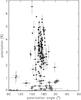 |
Fig. 1 Position angle vs. degree of polarization plot of 127 stars toward L1570 shown using filled circles. The open squares represent stars chosen from a circular area of radius 10° about L1570 obtained from Heiles (2000). |
3.2. Photometry
Results obtained from our BVRI photometry of stars toward L1570 are presented in Table 6. We found a total of 144 stars in the observed field with their photometric errors  0.1 mag in BVRIJHKs-bands. The JHKs magnitudes of the stars are obtained from the 2MASS. The unique star ids, their magnitudes and corresponding errors in BVRIJHKs-bands are tabulated in Table 6. Among these, 29 stars are found to have both polarimetric and photometric data. These stars are identified in Table 6 with their corresponding identification number from Table 2 (polarimetric results) shown in parenthesis.
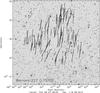 |
Fig. 2 Polarization vectors overplotted on the DSS B-band image of the field containing L1570. The length of the vectors corresponds to the degree of polarization and the direction of the orientation corresponds to the polarization position angle of stars measured from north increasing toward east. |
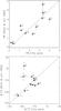 |
Fig. 3 P% (upper panel) and θ (lower panel) of stars toward L1570 from Bhatt & Jain (1993) (observed without any filter) are compared with those from this work (R-band). The stars are marked with their identification numbers taken from Table 2. Star #97 scattered more from the straight line is found to show (a) Hα emission in its spectra (Sect. 3.3); (b) NIR-excess (Sect. 4.2.1); and (c) intrinsic polarization and polarization angles (Sect. 4.2.1). |
3.3. Spectroscopy
Spectra of the two Hα sources, previously recognized by Ogura & Hasegawa (1983) and by Kohoutek & Wehmeyer (1997, 1999), are shown in Fig. 4. These sources are identified with 2MASS J06071585+1930001 (star #48 in Table 2, upper panel) and 2MASS J06075075+1934177 (star #97, lower panel). These stars are located in the western and northeastern parts of L1570, respectively. We classified these stars as a K4Ve and B4Ve type by comparing their spectrum with those from the stellar library provided by Jacoby et al. (1998). The presence of Hα in emission in these two stars is confirmed with an equivalent width of − 44 Å and − 83 Å for stars #48 and #97, respectively. It is interesting to note that star #97 shows some of the prominent diffused interstellar bands (DIBs) that are identified and labeled in the spectrum with their wavelengths taken from Herbig (1995). Just for comparison, we overplotted the spectrum of the star HD 189944 with spectral type B4V and E(B − V) = 0.065 (Neckel et al. 1980), obtained from the Indo-US library of coude-feed stellar spectra provided by Valdes et al. (2004), in gray in Fig. 4.
4. Discussion
4.1. Determination of distance to L1570
To subtract interstellar contribution from the observed polarization values, we required to know the distance to L1570. Previous estimates of distances to L1570 were highly uncertain. While Tomita et al. (1979) estimated a distance of 300 pc based on a star-count method, Bok & McCarthy (1974) assumed a distance of 400 pc to L1570 based on the number of stars brighter than mpg = 21 mag projected on the cloud in their photographic plate. Apart from these, no reliable distance estimates are available for L1570 in the literature. Most of the techniques used to determine distances to molecular clouds are in general extremely tedious and require a considerable amount of telescope time. We used the NIR photometric method presented in Maheswar et al. (2010), which uses the vast homogeneous JHKs photometric data produced by the 2MASS that is available for the entire sky, to determine the distance to L1570. Colors in the optical wavelengths also could have been used to determine the distance, but because we have observations of only the central region of L1570, the stars with optical photometry are not sufficient for the purpose.
A brief discussion of the method1 is presented below. It is based on a technique that allows spectral classification of stars lying toward the fields containing the clouds into main sequence and giants. In this technique the observed (J − H) and (H − Ks) colors of the stars with (J − Ks) ≤ 0.75 in (J − H) vs. (H − Ks) color–color (CC) diagram are de-reddened simultaneously using trial values of AV and a normal interstellar extinction law (i.e., total-to-selective extinction value, RV = 3.1)2. The best fit of the de-reddened colors to the intrinsic colors that gives a minimum value of χ2 then yields the corresponding spectral type and AV for the star. The main-sequence stars, thus classified, are then used in an AV versus distance plot to bracket the cloud distance. The entire procedure is illustrated in Fig. 5, where we plot the near-infrared CC (NIR-CC) diagram for the stars (with AV ≥ 1) chosen from the region F1 toward the direction of L1570 (see Fig. 6). The arrows are drawn from the observed data points (open circles) to the corresponding de-reddened colors estimated using the method. The highest extinction values that can be measured using the method are those for A0V type stars (≈4 mag). The extinction traced by stars will decrease as we move toward more late-type stars.
Details of the fields used for estimating the distance to L1570.
The giants located relatively far away distances if wrongly classified as main sequence, then they fall at closer distances with relatively high extinction values. This could lead to confusion on whether the increase in the extinction is caused by such spurious values or a cloud. We can overcome this difficulty by sub-dividing the field containing the cloud into smaller fields. While the rise in extinction due to a cloud should occur almost at the same distance in all fields, the mis-classified stars in the sub-fields would show high extinction not at same but at random distances if the whole cloud is located at the same distance. For cores with small angular sizes, we included fields containing additional cores that are located spatially closer and show similar radial velocities, to have a sufficient number of stars to infer their distances. Here we assume that the cores that are spatially closer, have similar velocities, and are located almost at the same distances.
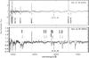 |
Fig. 4 Spectra of the stars 2MASS J06071585+1930001 (star #48, upper panel) and 2MASS J06075075+1934177 (star #97, lower panel). These two stars show Hα in emission. We found a number of DIBs in the spectrum of #97 that are identified and labeled. The spectrum of star HD 189944, with spectral type of B4V and E(B − V) = 0.065 (Neckel et al. 1980), obtained from the Indo-US library of coude-feed stellar spectra provided in Valdes et al. (2004), is overplotted in gray on the spectrum of #97 for a better identification of the DIBs. |
Kawamura et al. (1998) have made a large-scale survey in 13CO (J = 1−0) of the Gemini and Auriga regions (170° < l ≤ 196° and −10° ≤ b < 10°) with velocity coverages of −30 < VLSR < +30 km s-1. Though they have not detected L1570 in their survey, they have detected a number of clouds with VLSR closer to that of −0.5 km s-1 of L1570 (Clemens & Barvainis 1988). We selected clouds located below l = 0° with VLSR ≤ ± 1 km s-1. In Table 5, we present the field identification number, central galactic coordinates, cloud names, and VLSR values as given in Kawamura et al. (1998) and the dark clouds associated with the regions. In Fig. 6, we identify three (F1-3) of the total six regions on 2.5° × 1.5° extinction map produced by Dobashi et al. (2005). Each field, F1-6, covered an area of 30′ × 30′. The J, H, and Ks magnitudes of the stars were obtained from the 2MASS catalog (Skrutskie et al. 2006). Only those stars with photometric errors (which include the corrected band photometric uncertainty, nightly photometric zero point uncertainty, and flat-fielding residual errors) ≤0.03 magnitude and the photometric quality flag of AAA in all the three filters, i.e., S/N > 10 were considered. The positions of L1570, L1576 and L1578 are identified and labeled. The contours are drawn at 1, 2, and 3 magnitude levels. The filled circles show the positions of stars classified as dwarfs used for estimating the distance.
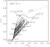 |
Fig. 5 (J − H) vs. (H − Ks) CC diagram drawn for stars (with AV ≥ 1) from F1 (see Fig. 6) region of L1570 to illustrate the method. The solid curve represents locations of unreddened main-sequence stars. The reddening vector for an A0V type star drawn parallel to the Rieke & Lebofsky (1985) interstellar reddening vector is shown with the dashed line. The locations of the main-sequence stars of different spectral types are marked with square symbols. The region to the right of the reddening vector is known as the NIR excess region and corresponds to the location of PMS sources. The dash-dot-dash line represents the loci of unreddened CTTSs (Meyer et al. 1997). The open circles represent the observed colors, and the arrows are drawn from the observed to the final colors obtained by the method for each star. |
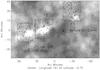 |
Fig. 6 2.5° × 1.5° extinction map produced by Dobashi et al. (2005) containing L1570 is shown with the fields F1-F3, each covering 30′ × 30′ area, marked and labeled. The contours are drawn at 1, 2 and 3 magnitude levels. The stars used for estimating the distance to L1570 are represented by filled circles. The clouds L1570, L1575, and L1578 are identified and labeled. |
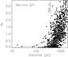 |
Fig. 7 AV vs. d plot for all stars obtained from the fields F1-F6 combined toward L1570. The dashed vertical line is drawn at 394 pc inferred from the procedure described in Maheswar et al. (2010, see the text for a brief description). The dash-dotted curve represents the increase in the extinction toward the Galactic latitude of b = −0.4591° as a function of distance produced from the expressions given in Bahcall & Soneira (1980). The error bars are not shown on all stars for clarity. |
In Fig. 7, we present the AV vs. d plot for all stars obtained from the fields F1-F6 combined toward L1570. The dash-dotted curve shows the increase in extinction toward the Galactic latitude of b = −0.4591° as a function of distance produced from the expressions given in Bahcall & Soneira (1980). The error bars are not drawn on all stars for clarity. A significant increase in the extinction is apparent at ~390 pc. To determine the distance to L1570, we first grouped the stars into distance bins of bin width = 0.18 × distance. The centers of each bin are separated by the half of the bin width. Since there exist very few stars at smaller distances, the mean value of the distances and the AV of the stars in each bin were calculated by taking 1000 pc as the initial point and proceeded toward smaller distances. The mean distance of the stars in the bin at which a significant drop in the mean of the extinction occurred was taken as the distance to the cloud and the average of the uncertainty in the distances of the stars in that bin was taken as the final uncertainty in distance determined by us for the cloud. The vertical dashed line in AV vs. d plots, used to mark the cloud distance, is drawn at the distance deduced from the above procedure. The error in the mean values of AV were calculated using the expression ![Mathematical equation: \hbox{$standard~deviation/\sqrt[]{N}$}](/articles/aa/full_html/2013/08/aa20603-12/aa20603-12-eq110.png) , where N is the number of stars in each bin. From the above procedure, we determined a distance of 394 ± 70 pc to L1570 (see Fig. 8).
, where N is the number of stars in each bin. From the above procedure, we determined a distance of 394 ± 70 pc to L1570 (see Fig. 8).
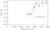 |
Fig. 8 Mean values of AV vs. the mean values of distance plot for L1570 produced using the procedure discussed in Maheswar et al. (2010, see text for a brief description). The distance at which the first sharp increase in the mean value of extinction occur is taken as the distance to the cloud. The error bars on the mean AV values were calculated using the expression |
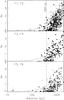 |
Fig. 9 AV vs. d plots for the stars from the fields F1-F6 toward L1570. The stars from the fields F1, F3, and F5 are shown with filled circles and those from F2, F4, and F6 are shown with open circles. The dashed vertical line is drawn at 394 pc inferred from the procedure described in Maheswar et al. (2010). The dash-dotted curve has the same meaning as in Fig. 7. |
In Fig. 9, we show AV vs. d plots for the stars from the individual fields F1-F6. The dash-dotted curve has the same meaning as in Fig. 7. The dashed vertical line is drawn at 394 pc. The stars from the fields F1, F3, and F5 are shown using filled circles and those from the fields F2, F4, and F6 are shown using open circles. In all six fields, the increase in the extinction significantly above the values expected from the expressions given in Bahcall & Soneira (1980) occurs consistently at or beyond ~390 pc. However, there exists evidence for a possible foreground dust layer at a distance of ~200 pc. On the basis of 338 stars that are selected from six fields and classified as dwarfs, we estimated a distance of 394 ± 70 pc to L1570.
4.2. Dust properties using polarimetric and photometric data
4.2.1. Pmax, λmax and RV values
Using our multi-wavelength data of the stars projected in the direction of L1570, we studied the properties of dust grains in the cloud. We obtained observations in V(RI)C filters for 42 stars and in B,V(RI)C filters for 15 stars. For our multi-wavelength observations we selected stars from various locations of the cloud so that the derived properties would represent the cloud as a whole.
We obtained Pmax and λmax using the weighted nonlinear least-squares fit to the measured polarization. We adopted K = 1.15 for stars with data in the V(RI)C pass-bands and K = 1.66 λmax + 0.01 (Whittet et al. 1992) for stars with data in the B,V(RI)C pass-bands. We also computed the parameters σ13, the unit weight error of the fit for each star, which quantifies the departure of the data from the standard Serkowski law and  , the dispersion of the polarization angle for each star normalized by the average of the polarization angle errors (cf. Marraco et al. 1993). The Serkowski parameters Pmax, λmax, σ1, and derived using V(RI)C4 wavelengths are given in Cols. 4 to 7 of Table 3 and those derived using B,V(RI)C are given in Cols. 4 to 7 of Table 4.
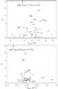 |
Fig. 10 Upper panel: σ1 vs. Pmax and lower panel: |
If the wavelength dependence of the polarization is well represented by the Serkowski law, σ1 should not exceed 1.5 because of the weighting scheme. A higher value (>1.5) could be indicative of intrinsic stellar polarization (Waldhausen et al. 1999; Feinstein et al. 2008; Eswaraiah et al. 2011, 2012, and references therein). The rotation of polarization angle with wavelength () also indicates an intrinsic polarization or a change of λmax along the line of sight (Coyne 1974; Martin 1974). Systematic variations with wavelength in the position angle of the interstellar linear polarization of star light may also be indicative of multiple dust layers with different magnetic field orientations along the line of sight (Messinger et al. 1997). Following these circumstances, we considered stars with σ1 > 1.5 and  (here, we considered only stars with values disagreeing with the normal distribution followed by the rest of the stars) as probable candidates to have either intrinsic polarization and/or rotation in the polarization angle. As shown in the upper and lower panels of the Fig. 10, we considered ten stars (#20, 23, 30, 47, 55, 56, 59, 83, 90, and 97) as candidates for either intrinsic polarization and/or rotation in their polarization angles.
Another criterion to detect intrinsic stellar polarization is based on the value of λmax. A star with λmax much lower than the average value of the ISM (0.545 μm; Serkowski et al. 1975) is considered as a candidate for an intrinsic component of polarization (Orsatti et al. 1998). In the present study we found only star #23 (whose σ1 = 16.9 and  ) with a much lower value of λmax = 0.33 ± 0.02 μm. We also considered the two stars #24 and #104 as peculiar because their λmax exceeds 0.85 μm.
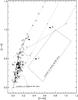 |
Fig. 11 (J − H) vs. (H − K) color–color diagram for all observed 127 stars of L1570 with either single R-band and or with VRI or BVRI data sets. The data are taken from the Cutri et al. (2003) catalog. The 2MASS data have been converted to the California Institute of Technology (CIT) system using the relations provided in Carpenter (2001). The theoretical tracks for dwarfs (thin line) and giants (thick line) are drawn (Bessell & Brett 1988). Reddening vectors (dashed lines) are also drawn (Cohen et al. 1981). The location of Be (cf. Dougherty et al. 1994) and of Herbig Ae/Be (cf. Hernández et al. 2005) stars are also shown. The stars with Hα emission in their spectra (labeled with their unique star id), the stars with probable intrinsic polarization and/or rotation in their polarization angles, and the stars with much lower or higher λmax are shown with filled circles. |
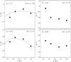 |
Fig. 12 Left panels: serkowski fit to the λ-dependent of polarization for stars #48 and #97. Right panels: λ-dependence of polarization angles for the same stars. |
The intrinsic polarization in a star could also be due to the asymmetric distribution of circumstellar material around the star in a disk or in a non-spherical envelope. Circumstellar material around a star is inferred from the NIR-CC diagram as shown in Fig. 11. We constructed the NIR-CC diagram using 2MASS JHKs magnitudes. The NIR excess sources occupy locations to the right of the reddening vector drawn for O-B spectral type stars. In Fig. 11, open circles represent the 127 stars observed by us. Only stars #48 and #97 (filled circles) clearly show NIR excess. Interestingly, stars #48 and #97 are located in regions generally occupied by classical T-Tauri and Herbig Ae/Be stars, respectively. In Fig. 12 we show the variation of the degree of polarization and position angle for #48 and #97 as a function of wavelength. As discussed earlier, both stars show intrinsic polarization and rotation in their polarization angle. In both the cases, the polarization angle seems to decrease with increasing wavelength, which is similar to observations in Messinger et al. (1997) toward the direction of Taurus dark cloud.
Based on the values of σ1, , i.e., with σ1 > 1.5 and/or ϵ> 4.0 and/or lower or higher values of λmax and/or the stars with possible NIR-excess based on NIR-CC diagram (Fig. 11), we identified 13 stars (#20, #23, #24, #30, #47, #48, #55, #56, #59, #83, #90, #97, and #104) with possible intrinsic polarization and/or rotation in their polarization angles. These stars were excluded from our study of dust properties of L1570. Figure 13 shows the frequency distribution of Pmax (upper panel) and λmax (lower panel) for 44 stars. The mean and standard deviation of Pmax and λmax was obtained with Gaussian fits to be 3.29 ± 0.91 per cent and 0.60 ± 0.05 μm, respectively. Using the relation RV = (5.6 ± 0.3) × λmax (Whittet & van Breda 1978), the value of RV is found to be 3.4 ± 0.3, which is slightly higher than the average value (RV = 3.1) for the Milky Way.
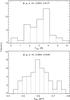 |
Fig. 13 Distribution of Pmax (upper panel) and λmax (lower panel) for 44 stars. The mean and standard deviation values obtained using Gaussian fits to the data are also indicated. |
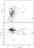 |
Fig. 14 Upper panel: degree of polarization in R-band vs. H − Ks color. Lower panel: polarization angle in R-band vs. H − Ks color. Horizontal dotted lines denote the Galactic parallel (GP) and the mean value of the polarization angles at 149° and 173°, respectively. The symbols are same as in Fig. 11. |
In Fig. 14 we show the plot between the polarization and the polarization angle versus H − Ks color for 114 stars. The thirteen stars with probable intrinsic polarization and (or) polarization angle rotation are shown with filled circles. As shown in the upper panel, the degree of polarization in R-band seems to increase with H − Ks color. This suggests that the main source of polarization is most likely the selective extinction by the aligned dust grains in the cloud. The lower panel suggests that the polarization angle for most stars is different from that of the Galactic parallel (149°) with a mean around 173°. However, there seems to be an indication that the position angles become aligned more with the Galactic parallel with increasing H − Ks color.
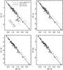 |
Fig. 15 (V − I), (V − J), (V − H), (V − K) vs. (B − V) two-color diagrams for the 135 stars (gray filled circles) with good photometric data (photometric errors <0.1 mag in BVRIJHK-bands) are plotted. The black filled circles denote 26 stars with both polarimetric and photometric data. The dashed lines are drawn using the color–color slopes mentioned in Table 7 to represent the normal reddening law, whereas the thick and gray straight lines denote the error-weighted straight line fits using 26 and 135 stars respectively. We excluded stars with possible intrinsic polarization (#48, #59, #83, #90, and #97) from this analysis. We also excluded four stars, #14, #42, #116, and #118, shown with filled star symbols, considering them as M-type dwarfs based on their location in the (V − I) vs. (B − V) plot. The thick curve shows the M-dwarf locus taken from Peterson & Clemens (1998). The reddening vector for a normal reddening law is drawn for AV = 2 mag. |
4.3. RV value based on two-color diagrams
The size of the dust grains can be constrained with the help of the parameter RV. The mean RV for the Milky-way Galaxy is found to be 3.1. But observationally it is found that the RV is not fixed but varies from one line of sight to the other. For example, toward the high-latitude translucent molecular cloud direction of HD 210121 (Larson et al. 1996), RV is found to be 2.1 whereas toward the HD 36982 molecular cloud direction in the Orion nebula the RV is found to be 5.6.
To investigate the nature of the extinction law in L1570, we used two-color diagrams (TCDs) as described by Pandey et al. (2000) and Pandey et al. (2003) in the form of (V − λ) versus (B − V), where λ is one of the wavelengths of the broad-band filters R, I, J, H, K, or L, to separate the influence of the normal extinction produced by the diffuse ISM with average dust grain size from that of the abnormal extinction arising within regions with a peculiar distribution of dust sizes (cf. Chini & Wargau 1990; Pandey et al. 2000). The (V − λ) versus (B − V) TCDs for the L1570 region are shown in Fig. 15. We found 144 stars with both optical (BVRI) and 2MASS (JHK) data with good photometric quality (photometric errors <0.1 mag in BVRIJHK-bands). To characterize the dust grain size using TCD, we used stars that are reddened by the cloud material. To exclude any un-reddened M-type dwarfs from our sample (which may contaminate the reddened sample), we superposed the locus of the M-type dwarfs (continuous curve) obtained from Peterson & Clemens (1998) in the (V − I) vs. (B − V) plot (top left panel). As shown in the top left panel, we identified four stars (#14, #42, #116, and #118 shown with filled star symbols) that are consistent with the intrinsic colors corresponding to the M-type dwarfs. However, the same un-reddened or reddened M-type dwarfs projected on the cloud could be used to determine a minimum distance to L1570 (Peterson & Clemens 1998). The reddening5 values for stars #14 and #46 are found to be 0.20 and 0.25 mag, respectively, whereas the reddening values for #116 and #118 are assumed to be 0.0 mag. The spectral types of these four stars are found to be M2.5V, M3V, M3V, and M3V. Using the absolute magnitudes, V-band magnitudes, and the reddening values, the distances are estimated as 68 pc, 239 pc, 190 pc, and 169 pc for stars #14, #42, #116, and #118, respectively. From this we conclude that L1570 is certainly located beyond ~240 pc.
Slopes of the color–color combination of the stars distributed toward L1570.
In addition to the five stars with possible intrinsic polarization (#48, #59, #83, #90, and #97), the four M-type stars (#14, #42, #116, and #118; shown with filled star symbols) are also excluded from the fit. Hence, out of 144 stars with photometric data, we used 135 stars (filled circles in gray) in TCD. Of these 135 stars, we found 26 stars with both polarimetric and photometric data (filled black circles). Error-weighted straight line fits were performed for the two-color distributions by using 26 and 135 stars separately, and the fitted slopes for each color-color distribution are mentioned in Table 7. In Fig. 15 the dotted line corresponds to the normal reddening law, whereas the gray and thick lines correspond to the error-weighted fitted slopes using the 26 and the 135 stars, respectively.
To derive the value of RV for the cloud region L1570, we used the approximate relation (see Neckel & Chini 1981),  (2)where mcloud and mnormal are the slopes of the two-color combination for the stars toward the cloud region and for the MS stars in the normal diffuse ISM (taken from the stellar models by Bertelli et al. 1994 and see also Table 3 of Pandey et al. 2003). Rnormal is taken as 3.1. Using the Eq. (2) and the slopes (cf. Table 7) for two cases with 26 and 135 stars, the weighted mean value of Rcloud is estimated to be 3.53 ± 0.02 and 3.64 ± 0.01. Within the error both sets of stars yield a similar value of RV, thereby indicating a possible anomalous reddening law toward L1570. The weighted mean of λmax (cf. Sect. 4.2.1) also indicated a slightly anomalous reddening law possibly because of bigger dust grains at the regions traced in our polarimetric and photometric observations.
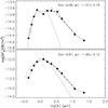 |
Fig. 16 Spectral energy distribution (log (λFλ) versus log (λ)) of stars #48 and #97 using non-simultaneous BVRI (see Table 6), JHKs (2MASS, Cutri et al. 2003) and WISE (Cutri et al. 2012) photometric data sets (filled circles). A straight line (dash line) is fitted to the data between 2 to 10 μm to derive the spectral index |

4.4. Spectral energy distribution of two Hα sources
We produced the spectral energy distribution (SED) for stars #48 and #97 using BVRI (our photometric observations), JHKs (2MASS; Cutri et al. 2003) and WISE (Cutri et al. 2012) photometric data. The SEDs thus produced are shown in Fig. 16. A straight line (dash line) is fitted to the data between 2 to 10 μm to find the spectral index  and to check whether these stars could possess any excess in the mid-infrared region of their SEDs because of the circumstellar disks around them. The α values of stars #48 and #97 are similar to those of a low-mass PMS star (CTTs/Class II) and an intermediate PMS star (HAe/Be) because their α values are − 1.01 ± 0.16 and − 1.82 ± 0.12. The classification scheme is adopted from Lada et al. (2006).
Bluer parts of the SEDs were closely matched with the reddened Kurucz model spectra (dotted curves) corresponding to the spectral types of K4V (upper panel) and B4V (lower panel). The model spectra were reddened using the following relation (Fitzpatrick & Massa 2007): 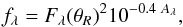 (3)where Fλ is the intrinsic stellar surface flux obtained from Kurucz models6, θR ≡ R/d is the stellar angular radius (where R is the radius of the star and d is the distance), and Aλ is the reddening at wavelength λ, which is represented using the mean RV-dependent extinction law of the form A(λ)/AV = a(x) + b(x)/RV (Cardelli et al. 1989). We used the following relation to estimate the scaling factor γ or
  , which uses the Kurucz model flux of the appropriate spectral type scaled to the observed visual magnitude (see Sujatha et al. 2004)
  (4)where K(5500 Å) is the Kurucz flux at 5500 Å, V is the V-band magnitude and τ = AV/1.0863. The SEDs of two stars were fitted visually for a given combination of spectral type (Kurucz model with temperature, gravity with solar metallicity), reddening E(B − V), RV (hence Aλ), and V-band magnitude. While star #48 was found to be best fitted at Teff = 4500 K, g = 4.5, E(B − V) = 0.265 and RV = 3.1, star #97 was found to be best fitted at Teff = 17 000 K, g = 4.0, E(B − V) = 1.21 and RV = 3.46, corresponding to spectral types of K4V and B4V, respectively. This is consistent with the spectral types derived from their respective spectra.
Using B and V magnitudes (from our photometry) and spectral types of K4V and B4V, we estimated a distance of ~400 pc for #48 (B = 17.33,V = 15.97,MV = 7.02,E(B − V) = 1.36−1.07 = 0.29,AV = 0.29 × 3.1 = 0.9) and ~1 kpc for #97 (B = 14.75,V = 13.41,MV = −1.52,E(B − V) = 1.34 + 0.19 = 1.53,AV = 1.53 × 3.1 = 4.74). Star #48 is probably located just in front of L1570 since the extinction toward this star of 0.9 mag is consistent with value expected at that distance (see Fig. 7) evaluated using the expression given in Bahcall & Soneira (1980). However, the exact nature of this star (whether a pre-main sequence or a normal emission type) is still unclear and requires further investigation. Star #97 clearly is a background star, which is supported by DIBs that are caused, most likely, by the material in the cloud.
4.5. Polarization efficiency
The polarization efficiency of the dust grains toward a particular direction/line of sight is defined as the degree of polarization produced for a given amount of extinction. The efficiency of polarization produced depends on the grain properties and the degree of alignment of these dust grains. Mie calculations for infinite cylindrical particles with dielectric optical properties that are perfectly aligned with their long axes parallel to each other and perpendicular to the line of sight place a theoretical upper limit on the polarization efficiency of the grains due to selective extinction. This upper limit is found to be P/AV ≤ 14% mag-1 (Whittet 2003). The observational upper limit on P/AV is found to be ≈3% mag-1 (Whittet 2003), however, a factor of four lower than the predicted value for the ideal scenario.
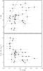 |
Fig. 17 Upper panel: plot of polarization degree (P) vs. total visual extinction (Av) derived from the method described in Sect. 4.1. We have selected only sources with Av/σAv ≥ 3. Lower panel: polarization efficiency (P/Av) vs. visual extinction Av. The solid line represents the observational upper limit of P/AV = 3. |
Using the method outlined in Sect. 4.1, we can estimate AV for a total of 82 stars. In Fig. 17 we present P versus AV (upper panel) and P/AV versus AV (lower panel) plots. We plotted only sources with Av/σAv ≥ 3. The plot of P versus AV (upper panel) shows that most of the data points lie on or below the line representing the usual relation P/AV ≈ 3% mag-1, implying that the characteristics of material composing L1570 is consistent with that of the diffuse ISM. The solid line represents the observational upper limit of P/AV = 3% mag-1. The plot in the lower panel shows that the polarization efficiency drops with increasing extinction.
4.6. Magnetic field geometry of L1570
Although the polarization of the stars located behind the cloud may be dominated by the dust associated with the cloud, the observed polarization will be a superposition of a component due to the dust located foreground to the cloud and another component due to the dust associated with the cloud. To evaluate the polarization produced only by the dust associated with the cloud, we need to subtract the foreground component from the observed polarization of the stars. This is essential to infer the true magnetic field orientation of the cloud and to study the magnetic field direction as a function of other cloud properties such as the structure, outflow directions, and the kinematics.
4.6.1. Foreground dust polarization
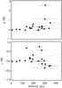 |
Fig. 18 q (upper panel) and u (lower panel) versus distance plots using the stars distributed in a circular radius of 10° about L1570. Straight line fits were performed to estimate the foreground Stokes parameters at the cloud possible minimum distance of 324 pc. 21 stars with available polarization measurements (Heiles 2000) and distance information (van Leeuwen 2007) were only used. Care was taken to not to include stars that show emission lines or are in binary systems as given in SIMBAD. |
One way to evaluate the foreground dust component is to determine the behavior of polarization with distance up to the distance of the cloud. Even though the distance and polarization information is known for 82 stars (Sect. 4.5) (whose distance values are well beyond ~400 pc), the distance values for four M-type stars (Sect. 4.3) are known (whose polarization data are not available) and the distance of one Hα emission star #48 is ~400 pc (Sect. 4.4) (which exhibits NIR-excess Fig. 11, intrinsic polarization and rotation in the polarization angles Fig. 12), none of these stars can be used to estimate the foreground polarization. Therefore, we searched for stars within a circular region of radius 10° about L1570 with polarization and distance measurements available in the literature. We obtained 21 stars with polarization measurements in the Heiles (2000) catalog. Care was taken to not to include stars that show emission lines or are in binary systems as given in SIMBAD. The distance to stars were estimated using the Hipparcos parallax measurements available in the catalog by van Leeuwen (2007). In Fig. 18, we show the values of the Stokes parameters q and u as a function of their distances. The uncertainty in our distance estimation of L1570 gives a minimum distance of 324 pc. Therefore we estimated the Stokes parameters qfg and ufg values representing the foreground dust component at 324 pc by making a fit to the data points as shown in Fig. 18. The estimated qfg and ufg at 324 pc are 0.3763% and 0.0625%, respectively. These values were subtracted from the corresponding Stokes parameters of our 127 objects to derive foreground-corrected qin and uin values. From these, we calculated the intrinsic degree of polarization and position angle for 127 objects. No significant change was noticed in the observed polarization results after correcting for the foreground contribution.
4.6.2. Magnetic field geometry
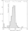 |
Fig. 19 Frequency distribution of polarization angles of 114 stars of L1570 after removing the foreground contribution. |
The mean value of the degree of polarization, after removing the foreground contribution as discussed in the previous section, is found to be 2.7% and a standard deviation of 1.2%. Figure 19 shows a peak in the distribution of polarization position angle centered on a mean of 171°, with a standard deviation of 8° obtained by making a Gaussian fit. The thirteen stars with evidence of an intrinsic component of polarization were excluded from the analysis. The dispersion in the position angles is found to be significantly lower, similar to the dispersion of position angles observed toward the bowl region of the Pipe nebula, which is suggested to be in a primordial evolutionary state (Alves et al. 2008).
In Fig. 20, we present the polarization map superposed on the false-color image of Herschel 250 micron SPIRE (Griffin et al. 2010) Photometer Short (250 μm) Wavelength Array (PSW) of the field containing L1570. The white contours represent the angular extent of the cloud in 250 μm. The minimum and maximum contour levels correspond to 0.08 Jy/beam and 8.55 Jy/beam, respectively. The contours indicate that the cloud is elongated along the north-south direction in a manner that the southern part of the cloud is oriented almost parallel to the Galactic parallel (~149° at b = −0.62°), whereas the northern part seems to be slightly bent toward the Galactic plane (b = 0°). The magnetic field geometry in L1570 also seems to follow the large-scale structure seen in Fig. 20. Toward the southern parts the field seems to be almost parallel to the Galactic parallel (~149° at b = −0.62°) and toward the northern parts the field lines are bent by ≈20° toward the Galactic plane (b = 0°) following the cloud structure.
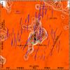 |
Fig. 20 Polarization vectors (blue) of 127 stars (after removing foreground contribution) are overplotted on the false-color image of Herschel 250 micron SPIRE (Griffin et al. 2010) Photometer Short (250 μm) Wavelength Array (PSW) of the field containing L1570. The length of the vectors corresponds to the degree of polarization, and the direction of the orientation corresponds to the polarization angle of the stars measured from the north increasing toward the east. A blue vector with a 3 percent polarization is drawn for reference. The white contours represent the dust emission at 250 μm at minimum and maximum levels of 0.08 Jy/beam and 8.55 Jy/beam, respectively. A color version of the figure is available in the online journal. |
The morphology of L1570 in the two-dimensional map of the cloud in 13CO made by Arquilla & Goldsmith (1985) looks very much similar to the one shown in the Fig. 20 (also see the 8 μm shadow image of L1570 produced by Spitzer telescope; Stutz et al. 2009). The velocity structure of L1570 by Arquilla & Goldsmith (1986) gives a complex picture of the region. L1570 consists of sub-condensations toward the north and the south-southeast of the main body. Along the declination strip, the northern condensation is prominent and along the northwest-southeast strip, the southern condensations are prominent. Based on their results, Arquilla & Goldsmith (1986) suggested that the velocity structure of L1570 originates from the fragmented nature of the gas complex with relative velocity differences of 0.5 km s-1 between the clumps. Also toward a number of positions in L1570, they identified secondary spectral features within 2 km s-1 of the L1570 main lines, indicating further fragmentation at scales that were not resolved in their observations. In Fig. 21, we show the central region of L1570 produced with Herschel with polarization vectors overplotted. The condensations identified initially by Arquilla & Goldsmith (1986) are clearly visible in Fig. 21. Both the northern and the southern condensations show filamentary structures. The filamentary structure seen toward the northern condensation seems to be aligned with the magnetic field lines.
The magnetic field geometry of a molecular cloud is mainly governed by the relative dynamical importance of magnetic forces to gravity, turbulence, and thermal pressure. If the magnetic fields are dynamically important, i.e., the support to the molecular cloud against gravity is provided predominantly by the magnetic field, then the field lines would be aligned smoothly and the mean field orientation would be perpendicular to the major axis of the cloud (Mouschovias 1978). This is expected as the cloud tends to contract more in the direction parallel to the magnetic field than in the direction perpendicular to it. On the other hand, if the magnetic fields are dynamically unimportant compared to the turbulence, the random motions dominate the structural dynamics of the clouds, and the field lines would be dragged around by turbulent eddies (Ballesteros-Paredes et al. 1999b). In that case, magnetic fields would be chaotic with no preferred direction.
In L1570, the relatively low dispersion in position angles implies that the magnetic field lines are aligned smoothly (see Fig. 19). The position angle of the major axis of the cloud is ~165° (inferred from the optical DSS images; Clemens & Barvainis 1988). Thus, the magnetic field lines in L1570 are oriented roughly parallel to the major axis in contrast to what is expected for a magnetic-field-dominated scenario. Ballesteros-Paredes et al. (1999a) and Hartmann et al. (2001) proposed that the molecular clouds are formed in large-scale, converging flows of diffuse atomic gas. Numerical simulations have shown that in a flow-driven cloud formation scenario, magnetic fields are believed to guide the flows to assemble the clouds whether through Parker instability (Parker 1966, 1967; Mouschovias et al. 1974, 2009), through turbulence in the ISM, or during the sweeping-up of gas in spiral shocks (Kim et al. 2006; Dobbs & Price 2008). Hartmann et al. (2001), based on the models of Passot et al. (1995), suggested that the field orientation with respect to the flows select the sites of cloud formation. The clouds will only form if the magnetic fields are aligned parallel to the flows. L1570 could have formed due to the converging flow of material along the field lines. This argument is supported by the orientation of filamentary structure along the field lines. The complex velocity structure in L1570 could be due to the collision of material in converging flows from opposite sides along the north-south direction guided by the magnetic field lines. Inference of velocity gradient in L1570 could confirm our argument. The magnetic field geometry of the high-density regions of L1570, where we see substructures, in near-infrared, or sub-millimeter wavelengths are highly desirable.
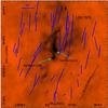 |
Fig. 21 Polarization vectors (blue) of 54 stars that are distributed in a 10 arcmin radius around the cloud center are overplotted on a false-color image of Herschel 250 micron SPIRE (Griffin et al. 2010) Photometer Short (250 μm) Wavelength Array (PSW) of the field containing L1570. The length of the vectors corresponds to the degree of polarization, and the direction of the orientation corresponds to the polarization angle of the stars measured from the north increasing toward the east. A blue vector with a 3 percent polarization is drawn for reference. A color version of the figure is available in the online journal. |
4.6.3. Magnetic field strength and cloud stability
To understand the cloud stability rendered by the magnetic fields against gravity and turbulence and to understand the importance of magnetic fields in cloud as well as star formation processes, it is crucial to estimate the magnetic field strength (Heitsch 2005).
The magnetic field strength can be derived by estimating the turbulent dispersion, spectral line-widths and the density. Using the dispersion in the polarization position angles in the modified Chandrasekhar-Fermi (CF) formula (Chandrasekhar & Fermi 1953; Ostriker et al. 2001), we estimated the plane of sky magnetic field strength. The value of n(H2) ≃ 598 cm-3 at 3 arc min distance (the distance at which the optical polarimetry is relevant) from the center of the cloud was adopted from Arquilla & Goldsmith (1985) and the line width value equal to 1.75 km s-1 found for CO toward the core (Clemens et al. 1991). Assuming these values, we found that the magnetic field strength in L1570 in the plane of sky is ≃80 μG.
However, the CF method assumes that the dispersion in the polarization angles is caused purely by hydrodynamic turbulence. This is not entirely true because other non-turbulent components such as cloud collapse, differential rotation, gravitational collapse, expanding Hii regions and, in addition, a component due to measurement error could also introduce the dispersion in the magnetic fields, as suggested by Hildebrand (2009), Hildebrand et al. (2009), and Hildebrand & Vaillancourt (2009). Moreover, it is hard to separate the turbulent dispersion from that due to large-scale structure (MHD waves along the spirals) and measurement errors.
The field strength can be estimated using the method (analogous to that used by CF) proposed by Hildebrand et al. (2009). This method essentially determines the angular dispersion due to turbulence in molecular clouds, where the turbulent dispersion is distinguishable from dispersion due to the large-scale structure or the apparent dispersion due to measurement error. To separate the turbulent from non-turbulent components, we plotted  (Falceta-Gonçalves et al. 2008; Franco et al. 2010; Poidevin et al. 2010; Santos et al. 2012, and references therein), the square root of the second-order structure function or angular dispersion function (ADF)7, as a function of distance (l) as shown in Fig. 22. We used the polarization angles of 127 stars to compute , which gives information on the behavior of the dispersion of the polarization angles as a function of the length scale in L1570. Recently, it has been used as a powerful statistical tool to infer information on the relationship between the large-scale and the turbulent components of the magnetic field in molecular clouds (see Hildebrand et al. 2009; Franco et al. 2010; Santos et al. 2012, and references therein).
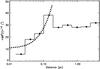 |
Fig. 22 Square root of the second-order structure function (or angular dispersion function (ADF)), |
The square of the dispersion function can be approximated as follows (Hildebrand et al. 2009): 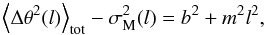 (5)where ⟨ Δθ2(l) ⟩ tot is the dispersion function computed from the data. The quantity σM2(l) is the measurement uncertainties, which is simply the average of the variances on Δθ(l) in each bin. The quantity b2 is the intercept of a straight line fit to the data (after subtracting σM2(l)). Hildebrand et al. (2009) have derived the equation for b2 to find the ratio of turbulent to the large-scale magnetic field strength:
 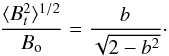 (6)In Fig. 22, we show the ADF versus distance for L1570 region. The errors in each bin are similar to the size of the symbols. Each bin denotes
 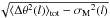 i.e., the ADF corrected for the measurement uncertainties. Bin widths are in logarithmic scale. Only four points were used in the linear fit to ensure that the length scale (l) used in the fit (0.015 to 0.20 pc) is greater than the turbulent length scale (δ) (which is on the order of 1 mpc or 0.001 pc; cf. Lazarian et al. 2004; Li & Houde 2008) and much shorter than the cloud length scale (d ~ 1 pc) i.e., δ < l ≪ d, to the data (Eq. (5)) versus distance squared. The fitted function is denoted with a thick dotted line. Since our optical polarimetric observations have a low resolution due to the available limited number of point sources, the minimum length we probed is ≃15 mpc. The turbulent contribution to the total ADF is determined by the zero intercept of the fit to the data at l = 0. The net turbulent component, b, is estimated to be 11° ± 3° (or 0.19 ± 0.06 rad). The ratio of the turbulent to large-scale magnetic field strength (
 ) is computed using Eq. (6) as 0.13 ± 0.04. This suggests that the turbulent component of the field is very small compared with the non-turbulent component, i.e., Bt ≪ B0. Based on this assumption, Hildebrand et al. (2009) showed that the uniform/non-turbulent component of the field can be approximated by the following relation:
 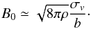 (7)As mentioned above, we used n(H2) ≃ 598 cm-3, velocity dispersion (σv) = 0.74 km s-1, and b = 11° ± 3°. The density can be estimated as ρ = n(H2)mHμH2, where n(H2) is the hydrogen column density, mH is the mass of the hydrogen atom, and μH2 ≈ 2.8 is the mean molecular weight per hydrogen molecule. Using these values, B0 is estimated to be ≃90 μG. Chapman et al. (2011, cf. their Eq. (7)) have used the following relation for estimating the dimensionless magnetic critical index in terms of total extinction AV (mag) and B0 (μG):
 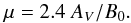 (8)Using the mean extinction for the L1570 region as AV = 1.77 mag8 and B0 ≃ 90 μG, we estimated μ as 0.047. If μ > 1, the cloud is assumed to be supercritical. If μ < 1, the cloud is said to be subcritical. The estimated value of μ for L1570 indicates that the cloud is magnetically subcritical, hence we infer that the cloud is supported by the magnetic fields. The value μ is also estimated using field strength B0 ≃ 80 μG (which is estimated using CF method) as 0.053. Thus, both the Hildebrand et al. and the CF method draw the similar conclusion that the cloud is subcritical.
5. Conclusions
We presented the results on dust properties and the magnetic field geometry toward the dark globule L1570 using multi-wavelength polarimetric and photometric observations. Our main conclusions are:
-
We estimated a distance of 394 ± 70 pc to thecloud using NIR photometry from 2MASS.
-
Based on our multi-wavelength polarimetric observations of 42 stars, the Serkowski parameters such as Pmax, λmax, and σ1 and a polarization angle rotation indicator,
, were determined. Stars with possible intrinsic polarization and (or) rotation in their position angles and (or) the stars with NIR-excess (based on their position in NIR color–color diagram) were identified. These stars were excluded from our study of the dust properties and the magnetic field geometry. -
The mean values of Pmax and λmax are found to be 3.29 ± 0.91 per cent and 0.60 ± 0.05 μm respectively, slightly higher than the value 0.545 μm corresponding to the general ISM. The value of RV estimated using the λmax is found to be 3.4 ± 0.3. Using (V − I), (V − J), (V − H), (V − K) vs. (B − V) two-color diagrams for the 135 stars, we evaluated the value of RV as 3.64 ± 0.01. The RV values derived from both these methods show that the grain size in L1570 is slightly bigger than those found in the diffuse ISM.
-
We confirmed the Hα emission features based on our spectroscopic observations of two stars, 2MASS J06071585+ 1930001 (#48) and 2MASS J06075075+1934177 (#97). These two stars were found to show NIR-excess as well. Star #97 shows some of the prominent DIBs in the spectrum. The spectral types of these stars are found to be K4Ve and B4Ve, respectively. We confirmed the spectral type determination of these sources by producing SEDs using optical, near- and far-IR data.
-
The magnetic field geometry of L1570 seems to follow the large-scale structure seen in the 250 μm image produced by Herschel. Toward the southern parts the field seems to be almost parallel to the Galactic parallel at b = −0.62°, whereas toward the northern parts the field lines are bent by ≈20° toward the Galactic plane (b = 0°). The filamentary structure seen toward the northern condensation are found to be aligned with the magnetic field lines. Based on the morphology of the magnetic field lines with respect to the cloud structure, we believe that L1570 could have formed due to the converging flow of material along the field lines. Using the dispersion in the polarization position angles in the modified Chandrasekhar-Fermi formula, we estimated the plane-of-sky magnetic field strength toward the outer parts of L1570 as ≃80 μG. Similarly, the structure function analysis yielded a magnetic field strength of ≃90 μG.
-
The structure function analysis suggests that the large-scale magnetic fields are stronger than the turbulent component of the magnetic fields in L1570 cloud region. The estimated magnetic field strengths using the Hildebrand et al. and the Chandrasekhar-Fermi method suggest that the L1570 cloud region is subcritical and hence probably is strongly supported by the magnetic field lines.
A more comprehensive discussion on the errors and limitations of the method can be found in Maheswar et al. (2010).
We derived the values of RV toward L1570 using polarimetric and photometric data in Sect. 4.2. Though there are hints of a slightly higher value of RV in L1570, we have chosen RV = 3.1 to determine the distance because the majority of the stars chosen around L1570 and other cloud regions (see Fig. 6) are from the periphery of the clouds and not from the higher extinction inner regions where higher RV values are usually found (e.g., Kandori et al. 2003).
The values of σ1 for each star were computed using the expression 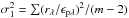 ; where m is the number of colors and rλ = Pλ − Pmaxexp [−K ln2(λmax/λ)].
To check the consistency in the values of Pmax and λmax derived using four data points and three data points, we derived the values of Pmax and λmax for 15 stars with B,V(RI)C data using V(RI)C only, i.e., excluding the B band data. The results were then compared with those obtained using the data from all four filters. The values obtained using the three and the four pass-band data are found to be consistent within the errors.
Reddening values are estimated by tracing back their (B − V) and (V − I) colors on to the intrinsic locus of M-type dwarfs by using the relations (B − V)0 = (B − V) − AV × RV; (V − I)0 = (V − I) −1.25AV × RV, where AV is the reddening and RV = 3.1 (which is valid for the diffuse ISM).
The Kurucz stellar flux can be obtained from: http://www.stsci.edu/science/starburst/Kurucz.html
The angular dispersion function (ADF) is defined as the square root to the average of the squared difference between the polarization angles measured for all pairs of points (N(l)) separated by a distance l.
We used only 34 stars, whose AV/σAV ≥ 3.0, to estimate the mean AV. See Sect. 4.5 for more details.
Acknowledgments
The authors are very grateful to the referee G. A. P. Franco for his insightful comments and suggestions, which helped considerably to improve the manuscript. This publication makes use of data products from the Two Micron All Sky Survey, which is a joint project of the University of Massachusetts and the Infrared Processing and Analysis Center/California Institute of Technology, funded by the National Aeronautics and Space Administration and the National Science Foundation. We also used images from the Digitized Sky Surveys, which were produced at the Space Telescope Science Institute under US Government grant NAG W-2166. The images of these surveys are based on photographic data obtained using the Oschin Schmidt Telescope on Palomar Mountain and the UK Schmidt Telescope. We acknowledge the use of NASA’s SkyView facility (http://skyview.gsfc.nasa.gov) located at NASA Goddard Space Flight Center. This research has also made use of the SIMBAD database, operated at CDS, Strasbourg, France.
References
- Alves, F. O., Franco, G. A. P., & Girart, J. M. 2008, A&A, 486, L13 [NASA ADS] [CrossRef] [EDP Sciences] [Google Scholar]
- Arquilla, R., & Goldsmith, P. F. 1985, ApJ, 297, 436 [NASA ADS] [CrossRef] [Google Scholar]
- Arquilla, R., & Goldsmith, P. F. 1986, ApJ, 303, 356 [NASA ADS] [CrossRef] [Google Scholar]
- Bahcall, J. N., & Soneira, R. M. 1980, ApJS, 44, 73 [NASA ADS] [CrossRef] [Google Scholar]
- Ballesteros-Paredes, J., Hartmann, L., & Vázquez-Semadeni, E. 1999a, ApJ, 527, 285 [NASA ADS] [CrossRef] [Google Scholar]
- Ballesteros-Paredes, J., Vázquez-Semadeni, E., & Scalo, J. 1999b, ApJ, 515, 286 [NASA ADS] [CrossRef] [Google Scholar]
- Basu, S. 2000, ApJ, 540, L103 [NASA ADS] [CrossRef] [Google Scholar]
- Bertelli, G., Bressan, A., Chiosi, C., Fagotto, F., & Nasi, E. 1994, A&AS, 106, 275 [NASA ADS] [Google Scholar]
- Bessell, M. S., & Brett, J. M. 1988, PASP, 100, 1134 [NASA ADS] [CrossRef] [Google Scholar]
- Bhatt, H. C., & Jain, S. K. 1992, MNRAS, 257, 57 [NASA ADS] [Google Scholar]
- Bhatt, H. C., & Jain, S. K. 1993, A&A, 276, 507 [NASA ADS] [Google Scholar]
- Bok, B. J., & Reilly, E. F. 1947, ApJ, 105, 255 [NASA ADS] [CrossRef] [Google Scholar]
- Bok, B. J., & McCarthy, C. C. 1974, AJ, 79, 42 [NASA ADS] [CrossRef] [Google Scholar]
- Cardelli, J. A., Clayton, G. C., & Mathis, J. S. 1989, ApJ, 345, 245 [NASA ADS] [CrossRef] [Google Scholar]
- Carpenter, J. M. 2001, AJ, 121, 2851 [NASA ADS] [CrossRef] [Google Scholar]
- Chandrasekhar, S., & Fermi, E. 1953, ApJ, 118, 116 [NASA ADS] [CrossRef] [MathSciNet] [Google Scholar]
- Chapman, N. L., Goldsmith, P. F., Pineda, J. L., et al. 2011, ApJ, 741, 21 [NASA ADS] [CrossRef] [Google Scholar]
- Chini, R., & Wargau, W. F. 1990, A&A, 227, 213 [NASA ADS] [Google Scholar]
- Clemens, D. P., & Barvainis, R. 1988, ApJS, 68, 257 [NASA ADS] [CrossRef] [Google Scholar]
- Clemens, D. P., Yun, J. L., & Heyer, M. H. 1991, ApJS, 75, 877 [NASA ADS] [CrossRef] [Google Scholar]
- Cohen, J. G., Persson, S. E., Elias, J. H., & Frogel, J. A. 1981, ApJ, 249, 481 [NASA ADS] [CrossRef] [Google Scholar]
- Coyne, G. V. 1974, AJ, 79, 565 [NASA ADS] [CrossRef] [Google Scholar]
- Coyne, G. V., Gehrels, T., & Serkowski, K. 1974, AJ, 79, 581 [NASA ADS] [CrossRef] [Google Scholar]
- Cutri, R. M., et al. 2012, VizieR Online Data Catalog: II/311 [Google Scholar]
- Cutri, R. M., Skrutskie, M. F., van Dyk, S., et al. 2003, VizieR Online Data Catalog: II/246 [Google Scholar]
- Davis, Jr., L., & Greenstein, J. L. 1951, ApJ, 114, 206 [Google Scholar]
- Dobashi, K., Uehara, H., Kandori, R., et al. 2005, PASJ, 57, 1 [Google Scholar]
- Dobbs, C. L., & Price, D. J. 2008, MNRAS, 383, 497 [NASA ADS] [CrossRef] [Google Scholar]
- Dougherty, S. M., Waters, L. B. F. M., Burki, G., et al. 1994, A&A, 290, 609 [NASA ADS] [Google Scholar]
- Eswaraiah, C., Pandey, A. K., Maheswar, G., et al. 2011, MNRAS, 411, 1418 [NASA ADS] [CrossRef] [Google Scholar]
- Eswaraiah, C., Pandey, A. K., Maheswar, G., et al. 2012, MNRAS, 419, 2587 [NASA ADS] [CrossRef] [Google Scholar]
- Falceta-Gonçalves, D., Lazarian, A., & Kowal, G. 2008, ApJ, 679, 537 [NASA ADS] [CrossRef] [Google Scholar]
- Feinstein, C., Vergne, M. M., Martínez, R., & Orsatti, A. M. 2008, MNRAS, 391, 447 [NASA ADS] [CrossRef] [Google Scholar]
- Fitzpatrick, E. L., & Massa, D. 2007, ApJ, 663, 320 [NASA ADS] [CrossRef] [EDP Sciences] [Google Scholar]
- Franco, G. A. P., Alves, F. O., & Girart, J. M. 2010, ApJ, 723, 146 [Google Scholar]
- Goldsmith, P. F., & Li, D. 2005, ApJ, 622, 938 [NASA ADS] [CrossRef] [Google Scholar]
- Goodman, A. A., Bastien, P., Menard, F., & Myers, P. C. 1990, ApJ, 359, 363 [NASA ADS] [CrossRef] [Google Scholar]
- Griffin, M. J., Abergel, A., Abreu, A., et al. 2010, A&A, 518, L3 [Google Scholar]
- Hartmann, L., Ballesteros-Paredes, J., & Bergin, E. A. 2001, ApJ, 562, 852 [NASA ADS] [CrossRef] [Google Scholar]
- Heiles, C. 2000, AJ, 119, 923 [NASA ADS] [CrossRef] [Google Scholar]
- Heitsch, F. 2005, in Astronomical Polarimetry: Current Status and Future Directions, eds. A. Adamson, C. Aspin, C. Davis, & T. Fujiyoshi, ASP Conf. Ser., 343, 166 [Google Scholar]
- Hennebelle, P., & Fromang, S. 2008, A&A, 477, 9 [NASA ADS] [CrossRef] [EDP Sciences] [Google Scholar]
- Herbig, G. H. 1995, ARA&A, 33, 19 [NASA ADS] [CrossRef] [Google Scholar]
- Hernández, J., Calvet, N., Hartmann, L., et al. 2005, AJ, 129, 856 [NASA ADS] [CrossRef] [Google Scholar]
- Hildebrand, R. H. 2009, in Submillimeter Astrophysics and Technology: a Symposium Honoring Thomas G. Phillips, eds. D. C. Lis, J. E. Vaillancourt, P. F. Goldsmith, T. A. Bell, N. Z. Scoville, & J. Zmuidzinas, ASP Conf. Ser., 417, 257 [Google Scholar]
- Hildebrand, R. H., & Vaillancourt, J. E. 2009, in Rev. Mex. Astron. Astrofis., Conf. Ser., 36, 137 [Google Scholar]
- Hildebrand, R. H., Kirby, L., Dotson, J. L., Houde, M., & Vaillancourt, J. E. 2009, ApJ, 696, 567 [NASA ADS] [CrossRef] [Google Scholar]
- Hilton, J., & Lahulla, J. F. 1995, A&AS, 113, 325 [NASA ADS] [Google Scholar]
- Jacoby, G. H., Hunter, D. A., & Christian, C. A. 1998, VizieR Online Data Catalog: III/092 [Google Scholar]
- Kandori, R., Dobashi, K., Uehara, H., Sato, F., & Yanagisawa, K. 2003, AJ, 126, 1888 [NASA ADS] [CrossRef] [Google Scholar]
- Kane, B. D., Clemens, D. P., Leach, R. W., & Barvainis, R. 1995, ApJ, 445, 269 [NASA ADS] [CrossRef] [Google Scholar]
- Kawamura, A., Onishi, T., Yonekura, Y., et al. 1998, ApJS, 117, 387 [NASA ADS] [CrossRef] [Google Scholar]
- Kim, C.-G., Kim, W.-T., & Ostriker, E. C. 2006, ApJ, 649, L13 [NASA ADS] [CrossRef] [Google Scholar]
- Kohoutek, L., & Wehmeyer, R. 1997, Catalogue of stars in the northern Milky Way having H-alpha in emission [Google Scholar]
- Kohoutek, L., & Wehmeyer, R. 1999, A&AS, 134, 255 [NASA ADS] [CrossRef] [EDP Sciences] [Google Scholar]
- Lada, C. J., Muench, A. A., Luhman, K. L., et al. 2006, AJ, 131, 1574 [NASA ADS] [CrossRef] [Google Scholar]
- Landolt, A. U. 1992, AJ, 104, 340 [NASA ADS] [CrossRef] [Google Scholar]
- Larson, K. A., Whittet, D. C. B., & Hough, J. H. 1996, ApJ, 472, 755 [NASA ADS] [CrossRef] [Google Scholar]
- Lazarian, A. 2003, J. Quant. Spec. Radiat. Transf., 79, 881 [Google Scholar]
- Lazarian, A., Vishniac, E. T., & Cho, J. 2004, ApJ, 603, 180 [NASA ADS] [CrossRef] [Google Scholar]
- Li, H.-B., & Houde, M. 2008, ApJ, 677, 1151 [NASA ADS] [CrossRef] [Google Scholar]
- Li, H., Dowell, C. D., Goodman, A., Hildebrand, R., & Novak, G. 2009, ApJ, 704, 891 [NASA ADS] [CrossRef] [Google Scholar]
- Lynds, B. T. 1962, ApJS, 7, 1 [NASA ADS] [CrossRef] [Google Scholar]
- Maheswar, G., Lee, C. W., Bhatt, H. C., Mallik, S. V., & Dib, S. 2010, A&A, 509, A44 [NASA ADS] [CrossRef] [EDP Sciences] [Google Scholar]
- Marraco, H. G., Vega, E. I., & Vrba, F. J. 1993, AJ, 105, 258 [NASA ADS] [CrossRef] [Google Scholar]
- Martin, P. G. 1974, ApJ, 187, 461 [NASA ADS] [CrossRef] [Google Scholar]
- McMillan, R. S. 1978, ApJ, 225, 880 [NASA ADS] [CrossRef] [Google Scholar]
- Medhi, B. J., Maheswar, G., Brijesh, K., et al. 2007, MNRAS, 378, 881 [NASA ADS] [CrossRef] [Google Scholar]
- Medhi, B. J., Maheswar, G., Pandey, J. C., Kumar, T. S., & Sagar, R. 2008, MNRAS, 388, 105 [NASA ADS] [CrossRef] [Google Scholar]
- Medhi, B. J., Maheswar, G., Pandey, J. C., Tamura, M., & Sagar, R. 2010, MNRAS, 403, 1577 [NASA ADS] [CrossRef] [Google Scholar]
- Messinger, D. W., Whittet, D. C. B., & Roberge, W. G. 1997, ApJ, 487, 314 [NASA ADS] [CrossRef] [Google Scholar]
- Meyer, M. R., Calvet, N., & Hillenbrand, L. A. 1997, AJ, 114, 288 [NASA ADS] [CrossRef] [Google Scholar]
- Mouschovias, T. C. 1978, in Protostars and Planets, ed. T. Gehrels, IAU Colloq., 52, 209 [Google Scholar]
- Mouschovias, T. C., & Spitzer, Jr., L. 1976, ApJ, 210, 326 [NASA ADS] [CrossRef] [Google Scholar]
- Mouschovias, T. C., Shu, F. H., & Woodward, P. R. 1974, A&A, 33, 73 [NASA ADS] [Google Scholar]
- Mouschovias, T. C., Kunz, M. W., & Christie, D. A. 2009, MNRAS, 397, 14 [NASA ADS] [CrossRef] [Google Scholar]
- Neckel, T., & Chini, R. 1981, A&AS, 45, 451 [NASA ADS] [Google Scholar]
- Neckel, T., Klare, G., & Sarcander, M. 1980, A&AS, 42, 251 [NASA ADS] [Google Scholar]
- Ogura, K., & Hasegawa, T. 1983, PASJ, 35, 299 [NASA ADS] [Google Scholar]
- Orsatti, A. M., Vega, E., & Marraco, H. G. 1998, AJ, 116, 266 [Google Scholar]
- Ostriker, E. C., Stone, J. M., & Gammie, C. F. 2001, ApJ, 546, 980 [NASA ADS] [CrossRef] [Google Scholar]
- Pandey, A. K., Ogura, K., & Sekiguchi, K. 2000, PASJ, 52, 847 [NASA ADS] [CrossRef] [Google Scholar]
- Pandey, A. K., Upadhyay, K., Nakada, Y., & Ogura, K. 2003, A&A, 397, 191 [NASA ADS] [CrossRef] [EDP Sciences] [Google Scholar]
- Parker, E. N. 1966, ApJ, 145, 811 [NASA ADS] [CrossRef] [Google Scholar]
- Parker, E. N. 1967, ApJ, 149, 517 [NASA ADS] [CrossRef] [Google Scholar]
- Passot, T., Vazquez-Semadeni, E., & Pouquet, A. 1995, ApJ, 455, 536 [NASA ADS] [CrossRef] [Google Scholar]
- Peterson, D. E., & Clemens, D. P. 1998, AJ, 116, 881 [NASA ADS] [CrossRef] [Google Scholar]
- Poidevin, F., Bastien, P., & Matthews, B. C. 2010, ApJ, 716, 893 [NASA ADS] [CrossRef] [Google Scholar]
- Rautela, B. S., Joshi, G. C., & Pandey, J. C. 2004, Bull. Astron. Soc. India, 32, 159 [Google Scholar]
- Rieke, G. H., & Lebofsky, M. J. 1985, ApJ, 288, 618 [NASA ADS] [CrossRef] [Google Scholar]
- Roberge, W. G. 2004, in Astrophysics of Dust, eds. A. N. Witt, G. C. Clayton, & B. T. Draine, ASP Conf. Ser., 309, 467 [Google Scholar]
- Santos, F. P., Roman-Lopes, A., & Franco, G. A. P. 2012, ApJ, 751, 138 [NASA ADS] [CrossRef] [Google Scholar]
- Schmidt, G. D., Elston, R., & Lupie, O. L. 1992, AJ, 104, 1563 [NASA ADS] [CrossRef] [Google Scholar]
- Serkowski, K., Mathewson, D. S., & Ford, V. L. 1975, ApJ, 196, 261 [NASA ADS] [CrossRef] [Google Scholar]
- Skrutskie, M. F., Cutri, R. M., Stiening, R., et al. 2006, AJ, 131, 1163 [NASA ADS] [CrossRef] [Google Scholar]
- Stutz, A. M., Rieke, G. H., Bieging, J. H., et al. 2009, ApJ, 707, 137 [NASA ADS] [CrossRef] [Google Scholar]
- Sujatha, N. V., Chakraborty, P., Murthy, J., & Henry, R. C. 2004, Bull. Astron. Soc. India, 32, 151 [Google Scholar]
- Tomita, Y., Saito, T., & Ohtani, H. 1979, PASJ, 31, 407 [NASA ADS] [Google Scholar]
- Valdes, F., Gupta, R., Rose, J. A., Singh, H. P., & Bell, D. J. 2004, ApJS, 152, 251 [NASA ADS] [CrossRef] [Google Scholar]
- van Leeuwen, F. 2007, A&A, 474, 653 [NASA ADS] [CrossRef] [EDP Sciences] [Google Scholar]
- Vrba, F. J., Strom, S. E., & Strom, K. M. 1976, AJ, 81, 958 [NASA ADS] [CrossRef] [Google Scholar]
- Waldhausen, S., Martínez, R. E., & Feinstein, C. 1999, AJ, 117, 2882 [NASA ADS] [CrossRef] [Google Scholar]
- Ward-Thompson, D., Sen, A. K., Kirk, J. M., & Nutter, D. 2009, MNRAS, 398, 394 [NASA ADS] [CrossRef] [Google Scholar]
- Whittet, D. C. B. 2003, Dust in the galactic environment (Bristol: IOP) [Google Scholar]
- Whittet, D. C. B., & van Breda, I. G. 1978, A&A, 66, 57 [NASA ADS] [Google Scholar]
- Whittet, D. C. B., Martin, P. G., Hough, J. H., et al. 1992, ApJ, 386, 562 [NASA ADS] [CrossRef] [Google Scholar]
- Wilking, B. A., Lebofsky, M. J., & Rieke, G. H. 1982, AJ, 87, 695 [NASA ADS] [CrossRef] [Google Scholar]
- Yun, J. L., & Clemens, D. P. 1990, ApJ, 365, L73 [NASA ADS] [CrossRef] [Google Scholar]
- Yun, J. L., & Clemens, D. P. 1992, ApJ, 385, L21 [NASA ADS] [CrossRef] [Google Scholar]
All Tables
All Figures
|
Fig. 1 Position angle vs. degree of polarization plot of 127 stars toward L1570 shown using filled circles. The open squares represent stars chosen from a circular area of radius 10° about L1570 obtained from Heiles (2000). |
| In the text | |
|
Fig. 2 Polarization vectors overplotted on the DSS B-band image of the field containing L1570. The length of the vectors corresponds to the degree of polarization and the direction of the orientation corresponds to the polarization position angle of stars measured from north increasing toward east. |
| In the text | |
|
Fig. 3 P% (upper panel) and θ (lower panel) of stars toward L1570 from Bhatt & Jain (1993) (observed without any filter) are compared with those from this work (R-band). The stars are marked with their identification numbers taken from Table 2. Star #97 scattered more from the straight line is found to show (a) Hα emission in its spectra (Sect. 3.3); (b) NIR-excess (Sect. 4.2.1); and (c) intrinsic polarization and polarization angles (Sect. 4.2.1). |
| In the text | |
|
Fig. 4 Spectra of the stars 2MASS J06071585+1930001 (star #48, upper panel) and 2MASS J06075075+1934177 (star #97, lower panel). These two stars show Hα in emission. We found a number of DIBs in the spectrum of #97 that are identified and labeled. The spectrum of star HD 189944, with spectral type of B4V and E(B − V) = 0.065 (Neckel et al. 1980), obtained from the Indo-US library of coude-feed stellar spectra provided in Valdes et al. (2004), is overplotted in gray on the spectrum of #97 for a better identification of the DIBs. |
| In the text | |
|
Fig. 5 (J − H) vs. (H − Ks) CC diagram drawn for stars (with AV ≥ 1) from F1 (see Fig. 6) region of L1570 to illustrate the method. The solid curve represents locations of unreddened main-sequence stars. The reddening vector for an A0V type star drawn parallel to the Rieke & Lebofsky (1985) interstellar reddening vector is shown with the dashed line. The locations of the main-sequence stars of different spectral types are marked with square symbols. The region to the right of the reddening vector is known as the NIR excess region and corresponds to the location of PMS sources. The dash-dot-dash line represents the loci of unreddened CTTSs (Meyer et al. 1997). The open circles represent the observed colors, and the arrows are drawn from the observed to the final colors obtained by the method for each star. |
| In the text | |
|
Fig. 6 2.5° × 1.5° extinction map produced by Dobashi et al. (2005) containing L1570 is shown with the fields F1-F3, each covering 30′ × 30′ area, marked and labeled. The contours are drawn at 1, 2 and 3 magnitude levels. The stars used for estimating the distance to L1570 are represented by filled circles. The clouds L1570, L1575, and L1578 are identified and labeled. |
| In the text | |
|
Fig. 7 AV vs. d plot for all stars obtained from the fields F1-F6 combined toward L1570. The dashed vertical line is drawn at 394 pc inferred from the procedure described in Maheswar et al. (2010, see the text for a brief description). The dash-dotted curve represents the increase in the extinction toward the Galactic latitude of b = −0.4591° as a function of distance produced from the expressions given in Bahcall & Soneira (1980). The error bars are not shown on all stars for clarity. |
| In the text | |
|
Fig. 8 Mean values of AV vs. the mean values of distance plot for L1570 produced using the procedure discussed in Maheswar et al. (2010, see text for a brief description). The distance at which the first sharp increase in the mean value of extinction occur is taken as the distance to the cloud. The error bars on the mean AV values were calculated using the expression |
| In the text | |
|
Fig. 9 AV vs. d plots for the stars from the fields F1-F6 toward L1570. The stars from the fields F1, F3, and F5 are shown with filled circles and those from F2, F4, and F6 are shown with open circles. The dashed vertical line is drawn at 394 pc inferred from the procedure described in Maheswar et al. (2010). The dash-dotted curve has the same meaning as in Fig. 7. |
| In the text | |
|
Fig. 10 Upper panel: σ1 vs. Pmax and lower panel: |
| In the text | |
|
Fig. 11 (J − H) vs. (H − K) color–color diagram for all observed 127 stars of L1570 with either single R-band and or with VRI or BVRI data sets. The data are taken from the Cutri et al. (2003) catalog. The 2MASS data have been converted to the California Institute of Technology (CIT) system using the relations provided in Carpenter (2001). The theoretical tracks for dwarfs (thin line) and giants (thick line) are drawn (Bessell & Brett 1988). Reddening vectors (dashed lines) are also drawn (Cohen et al. 1981). The location of Be (cf. Dougherty et al. 1994) and of Herbig Ae/Be (cf. Hernández et al. 2005) stars are also shown. The stars with Hα emission in their spectra (labeled with their unique star id), the stars with probable intrinsic polarization and/or rotation in their polarization angles, and the stars with much lower or higher λmax are shown with filled circles. |
| In the text | |
|
Fig. 12 Left panels: serkowski fit to the λ-dependent of polarization for stars #48 and #97. Right panels: λ-dependence of polarization angles for the same stars. |
| In the text | |
|
Fig. 13 Distribution of Pmax (upper panel) and λmax (lower panel) for 44 stars. The mean and standard deviation values obtained using Gaussian fits to the data are also indicated. |
| In the text | |
|
Fig. 14 Upper panel: degree of polarization in R-band vs. H − Ks color. Lower panel: polarization angle in R-band vs. H − Ks color. Horizontal dotted lines denote the Galactic parallel (GP) and the mean value of the polarization angles at 149° and 173°, respectively. The symbols are same as in Fig. 11. |
| In the text | |
|
Fig. 15 (V − I), (V − J), (V − H), (V − K) vs. (B − V) two-color diagrams for the 135 stars (gray filled circles) with good photometric data (photometric errors <0.1 mag in BVRIJHK-bands) are plotted. The black filled circles denote 26 stars with both polarimetric and photometric data. The dashed lines are drawn using the color–color slopes mentioned in Table 7 to represent the normal reddening law, whereas the thick and gray straight lines denote the error-weighted straight line fits using 26 and 135 stars respectively. We excluded stars with possible intrinsic polarization (#48, #59, #83, #90, and #97) from this analysis. We also excluded four stars, #14, #42, #116, and #118, shown with filled star symbols, considering them as M-type dwarfs based on their location in the (V − I) vs. (B − V) plot. The thick curve shows the M-dwarf locus taken from Peterson & Clemens (1998). The reddening vector for a normal reddening law is drawn for AV = 2 mag. |
| In the text | |
|
Fig. 16 Spectral energy distribution (log (λFλ) versus log (λ)) of stars #48 and #97 using non-simultaneous BVRI (see Table 6), JHKs (2MASS, Cutri et al. 2003) and WISE (Cutri et al. 2012) photometric data sets (filled circles). A straight line (dash line) is fitted to the data between 2 to 10 μm to derive the spectral index |
| In the text | |
|
Fig. 17 Upper panel: plot of polarization degree (P) vs. total visual extinction (Av) derived from the method described in Sect. 4.1. We have selected only sources with Av/σAv ≥ 3. Lower panel: polarization efficiency (P/Av) vs. visual extinction Av. The solid line represents the observational upper limit of P/AV = 3. |
| In the text | |
|
Fig. 18 q (upper panel) and u (lower panel) versus distance plots using the stars distributed in a circular radius of 10° about L1570. Straight line fits were performed to estimate the foreground Stokes parameters at the cloud possible minimum distance of 324 pc. 21 stars with available polarization measurements (Heiles 2000) and distance information (van Leeuwen 2007) were only used. Care was taken to not to include stars that show emission lines or are in binary systems as given in SIMBAD. |
| In the text | |
|
Fig. 19 Frequency distribution of polarization angles of 114 stars of L1570 after removing the foreground contribution. |
| In the text | |
|
Fig. 20 Polarization vectors (blue) of 127 stars (after removing foreground contribution) are overplotted on the false-color image of Herschel 250 micron SPIRE (Griffin et al. 2010) Photometer Short (250 μm) Wavelength Array (PSW) of the field containing L1570. The length of the vectors corresponds to the degree of polarization, and the direction of the orientation corresponds to the polarization angle of the stars measured from the north increasing toward the east. A blue vector with a 3 percent polarization is drawn for reference. The white contours represent the dust emission at 250 μm at minimum and maximum levels of 0.08 Jy/beam and 8.55 Jy/beam, respectively. A color version of the figure is available in the online journal. |
| In the text | |
|
Fig. 21 Polarization vectors (blue) of 54 stars that are distributed in a 10 arcmin radius around the cloud center are overplotted on a false-color image of Herschel 250 micron SPIRE (Griffin et al. 2010) Photometer Short (250 μm) Wavelength Array (PSW) of the field containing L1570. The length of the vectors corresponds to the degree of polarization, and the direction of the orientation corresponds to the polarization angle of the stars measured from the north increasing toward the east. A blue vector with a 3 percent polarization is drawn for reference. A color version of the figure is available in the online journal. |
| In the text | |
|
Fig. 22 Square root of the second-order structure function (or angular dispersion function (ADF)), |
| In the text | |
Current usage metrics show cumulative count of Article Views (full-text article views including HTML views, PDF and ePub downloads, according to the available data) and Abstracts Views on Vision4Press platform.
Data correspond to usage on the plateform after 2015. The current usage metrics is available 48-96 hours after online publication and is updated daily on week days.
Initial download of the metrics may take a while.