| Issue |
A&A
Volume 555, July 2013
|
|
|---|---|---|
| Article Number | A43 | |
| Number of page(s) | 13 | |
| Section | Extragalactic astronomy | |
| DOI | https://doi.org/10.1051/0004-6361/201220828 | |
| Published online | 27 June 2013 | |
The XMM deep survey in the CDF-S
IV. Compton-thick AGN candidates
1 INAF – Osservatorio Astronomico di Bologna, via Ranzani 1, 40127 Bologna, Italy
e-mail: ioannis.georgantopoulos@oabo.inaf.it
2 Institute of Astronomy & Astrophysics, National Observatory of Athens, Palaia Penteli, 15236 Athens, Greece
3 Physics & Astronomy Department, University of Bologna, Viale Berti Pichat 6/2, 40127 Bologna, Italy
4 Physics Department, University of Durham, South Road, Durham, DH1 7RH, UK
5 ICREA and Institut de Ciéncies del COSMOS (ICC), Universitat de Barcelona (IEEC-UB), Martí i Franqués 1, 08028 Barcelona, Spain
6 Instituto de Fisica de Cantabria (CSIC-Universidad de Cantabria), 39005 Santander, Spain
7 INAF – Osservatorio Astronomico di Padova, Vicolo dell’Osservatorio 5, 35122 Padova, Italy
8 Irfu/Service Astrophysique, CEA-Saclay, Orme des Merisiers, 91191 Gif-sur-Yvette Cedex, France
9 INAF Osservatorio Astronomico di Trieste, via G.B. Tiepolo 11, 34143 Trieste, Italy
10 Max Planck für Extraterrestrische Physik, Karl Schwarzschild strasse, 85748 Garching, Germany
Received: 30 November 2012
Accepted: 21 March 2013
The Chandra Deep Field is the region of the sky with the highest concentration of X-ray data available: 4 Ms of Chandra and 3 Ms of XMM-Newton data, allowing excellent quality spectra to be extracted even for faint sources. We took advantage of this to compile a sample of heavily obscured active galactic nuclei (AGN) using X-ray spectroscopy. We selected our sample among the 176 brightest XMM-Newton sources, searching for either flat X-ray spectra (Γ < 1.4 at the 90% confidence level) suggestive of a reflection dominated continuum or an absorption turn-over suggestive of a column density higher than ≈ 1024 cm-2. We found a sample of nine heavily-obscured sources satisfying the above criteria. Four of these show statistically significant FeKα lines with large equivalent widths (three out of four have equivalent widths consistent with 1 keV) suggesting that these are the most certain Compton-thick AGN candidates. Two of these sources are transmission dominated while the other two are most probably reflection dominated Compton-thick AGN. Although this sample of four sources is by no means statistically complete, it represents the best example of Compton-thick sources found at moderate-to-high redshift with three sources at z = 1.2–1.5 and one source at z = 3.7. Using Spitzer and Herschel observations, we estimate with good accuracy the X-ray to mid-IR (12 μm) luminosity ratio of our sources. These are well below the average AGN relation, independently suggesting that these four sources are heavily obscured.
Key words: X-rays: diffuse background / infrared: galaxies / galaxies: active / X-rays: galaxies
© ESO, 2013
1. Introduction
The nature of the X-ray background (XRB) has been contentious since its discovery 50 years ago (Giacconi et al. 1962). The Chandra mission confirmed that the background is made up of the summed emission from active galactic nuclei (AGN; Brandt & Hasinger 2005). The resolved fraction of the XRB is about ~90% in the 0.5–2 keV and 2–5 keV bands (Alexander et al. 2003; Xue et al. 2011). Optical spectroscopic follow-up observations show that the peak of the redshift distribution of these sources is at z ~ 0.7 − 1 (Barger et al. 2003; Silverman et al. 2010). At higher energies, the limited sensitivity hampers the resolution of a large fraction of the XRB. Narrow energy-band source stacking shows that this fraction reduces to ~60% over 5−8 keV, and only ~50% above 8 keV (Worsley et al. 2005, 2006; Xue et al. 2012; Moretti et al. 2012).
Still, it is at high energies where the bulk of the XRB energy density is produced. The peak of the X-ray background at 20–30 keV (e.g. Frontera et al. 2007; Churazov et al. 2007; Moretti et al. 2009) can be reproduced only by invoking a significant number of heavily obscured and Compton-thick AGN. Compton-thick AGN are those where the absorbing column densities exceed 1.5 × 1024 cm-2 and thus the attenuation of X-rays by photoelectric absorption is enhanced by the scattering on electrons (for reviews on Compton-thick AGN properties and surveys see Comastri 2004; Georgantopoulos 2012). However, the exact density of heavily obscured AGN required by X-ray background synthesis models is still under dispute (Gilli et al. 2007; Sazonov et al. 2008; Treister et al. 2009a; Ballantyne et al. 2011; Akylas et al. 2012). In particular, the intrinsic fraction of Compton-thick AGN may vary from 15 to over 35% (see discussion in Akylas et al. 2012). Additional evidence of a numerous Compton-thick population comes from the directly measured space density of black holes in the local Universe (see Soltan 1982). It is found that this space density is a factor of 1.5–2 higher than predicted by the X-ray luminosity function (Marconi et al. 2004; Merloni & Heinz 2008), although the exact number depends on the assumed efficiency in the conversion of gravitational energy to radiation.
The advent of the INTEGRAL and Swift missions helped to constrain the Compton-thick population in the local Universe. These missions explored the X-ray sky at energies above 10 keV probably providing the most unbiased samples of Compton-thick AGN over the whole sky. Owing to the limited imaging capabilities of these missions (carrying coded-mask detectors), the flux limit probed is bright (f15 − 55 keV ~ 10-11 erg cm-2 s-1), allowing only the detection of AGN at very low redshifts. These ultra-hard surveys did not detect large numbers of Compton-thick sources (e.g. Ajello et al. 2008; Tueller et al. 2008; Paltani et al. 2008; Winter et al. 2009; Burlon et al. 2011; Malizia et al. 2012; Goulding et al. 2011). The fraction of Compton-thick AGN in these surveys does not exceed a few percent of the total AGN population. In contrast, optical and mid-IR surveys yield Compton-thick AGN fractions of between 10% and 20% (Akylas & Georgantopoulos 2009; Brightman & Nandra 2011). However, even the ultra-hard surveys may miss a fraction of Compton-thick AGN, i.e. those with NH > 2 × 1024 cm-2. As Burlon et al. (2011) point out, this may explain the relative scarcity of Compton-thick AGN found in the ultra-hard INTEGRAL and Swift surveys.
At higher redshifts, a number of efforts have been made to identify Compton-thick AGN. For example, Gilli et al. (2010) provide samples of Compton-thick AGN at moderate redshifts (z ~ 1) using optical spectroscopy and in particular the [NeV] emission line. Searches for high-redshift Compton-thick AGN in the mid-IR also attracted much interest, mainly because the absorbed radiation heats the surrounding material and is re-emitted at IR wavelengths. The techniques that have been employed include the detection of a high 24 μm emission relative to the optical emission (e.g. Fiore et al. 2008, 2009; Georgantopoulos et al. 2008; Treister et al. 2009b; Eckart et al. 2010), and the presence of a low X-ray-to-mid-IR luminosity ratio (see Alexander et al. 2008, 2011; Georgantopoulos et al. 2011b) Most recently, Georgantopoulos et al. (2011a) proposed the presence of deep silicate features in mid-IR Spitzer spectra, although Goulding et al. (2012) argue that the silicate absorption in these sources is related to the host galaxies. Nevertheless, the most unambiguous method for finding Compton-thick sources relies on X-ray spectroscopy. In X-ray wavelengths, the most systematic attempts include these by Tozzi et al. (2006); Georgantopoulos et al. (2007, 2009), and more recently Brightman & Ueda (2012) all in the Chandra deep fields. A number of Compton-thick sources have been individually discussed in Norman et al. (2002), Iwasawa et al. (2005), Comastri et al. (2011), Feruglio et al. (2011), Gilli et al. (2011), Georgantopoulos et al. (2011b), and Iwasawa et al. (2012a). In particular, Comastri et al. (2011) has provided the most direct X-ray spectroscopic evidence yet for the presence of Compton-thick nuclei at high redshift, reliably identifying two Compton-thick AGN at z = 1.536 and z = 3.700.
Here, we attempt to find unambiguous examples of Compton-thick AGN at moderate redshifts, extending the work of Comastri et al. (2011). The Chandra Deep Field South (CDF-S) is one of the regions of the sky with the largest accumulation of multi-wavelength data available. In particular, it is the area with the most sensitive X-ray observations, namely 3 Ms of XMM-Newton data and 4 Ms of Chandra data, allowing the extraction of good quality X-ray spectra even for faint X-ray sources such as heavily obscured AGN. Owing to the superior XMM-Newton photon collecting power, we first select a sample of heavily obscured AGN using the 3 Ms XMM-Newton observations. For these sources, we present a combined XMM-Newton and Chandra spectral analysis to increase the photon statistics. Our aim is to detect unambiguous signs of Compton-thick obscuration, such as direct detection of a large column density, or a flat spectral index, and finally a large equivalent-width (hereafter EW) Fe Kα line. Finally, we examine the mid-IR and far-IR (up to rest-frame wavelengths of 160 μm) properties of our sources using data from the Spitzer and Herschel missions. The aim is to check whether the IR observations independently support a heavy obscuration scenario. We adopt Ho = 75 km s-1 Mpc-1, ΩM = 0.3, and ΩΛ = 0.7 throughout the paper.
2. Data
2.1. X-ray
2.1.1. XMM-Newton
The CDF-S area was surveyed with XMM-Newton during different epochs spread over almost nine years. The data presented in this paper were obtained by combining the observations awarded to our project and observed between July 2008 and March 2010 (Comastri et al. 2011) with the archival data acquired in the period July 2001–January 2002. The total exposure time, after the removal of background flares, is ≈2.82 Ms for the two MOS and ≈2.45 Ms for the PN detectors. The total area covered is 30 × 35 arcmin. The source catalogue contains 339 X-ray sources detected in the 2–10 keV band with a significance larger than 5σ and a flux density limit of ≈6.6 × 10⁻¹⁶ erg cm-2 s-1 assuming Γ = 1.7. A supplementary list of 74 sources detected with lesser significance is also provided. An extended and detailed description of the full data set, including data analysis and reduction and the X-ray catalogue, will be published in Ranalli et al. (2013).
2.1.2. Chandra
The CDF-S 4 Ms observations consist of 53 pointings obtained in the years 2000 (1 Ms), 2007 (1 Ms), and 2010 (2 Ms). The analysis of the first 1 Ms data is presented in Giacconi et al. (2002) and Alexander et al. (2003), while the analysis of the 23 observations obtained up to 2007 is presented in Luo et al. (2008). In the present 4 Ms survey, 740 sources are detected down to a sensitivity limit of ~ 0.7 × 10⁻¹⁶ erg cm-2 s-1 and 1 × 10-17 erg cm-2 s-1 in the hard (2–8 keV) and soft (0.5–2 keV) band, respectively (Xue et al. 2011). The Galactic column density towards the CDF-S is 0.9 × 1020 cm-2 (Dickey & Lockman 1990).
2.2. Infrared
2.2.1. Spitzer
The central regions of the CDF-S were observed in the mid-IR by the Spitzer mission as part of the Great Observatories Origins Deep Survey (GOODS). These observations cover areas of about 10 × 16.5 arcmin2 using the IRAC (3.6, 4.5, 5.8, and 8.0 μm) bands. These data are combined with more recent observations of the wider E-CDF-S area in the SIMPLE survey (Damen et al. 2011). The combined data-set has a 5σ magnitude limit of [3.6 μm] AB = 23.86, while the 3σ magnitude limit of the central GOODS region is [3.6 μm]AB = 26.15. The GOODS area in the centre of the CDF-S has also been imaged with the MIPS detector onboard Spitzer in the 24 μm band with a 5σ flux density limit of 30 μJy. A much wider area, including the entire E-CDF-S was imaged as part of the FIDEL legacy program (Magnelli et al. 2009) with a 5σ flux density limit of 70 μJy; we use a combination of the two data-sets for this work.
2.2.2. Herschel
The far-Infrared data in this work come from the GOODS-Herschel survey of Elbaz et al. (2010). This is the deepest survey of Herschel using the PACS instrument in both the 100 and the 160 μm bands, with an integration time of more than 15 h per position. The area covered is a 13 × 11 arcmin field inside the GOODS area. The source detection is performed using a 24 μm prior position and the 3σ flux density limits are 0.8 and 2.4 mJy in the 100 and 160 μm bands respectively. The GOODS-Herschel catalogue we use also utilises public data from the HerMES survey (Oliver et al. 2012) in the CDF-S. We use a 250 μm catalogue based on 24 μm prior positions covering the GOODS-S area, and we keep sources with a flux density determination better than the 2σ limit of 3.5 mJy.
3. Sample definition and X-ray spectral extraction
3.1. The sample
We confine our analysis to the brightest sources in the preliminary XMM-Newton catalogue, i.e. those with a detection probability of 8σ. There are 194 sources from both the main and supplementary lists satisfying the above criterion. However, for a number of sources we cannot derive an XMM-Newton spectrum in any of the cameras, either because they are too faint (they lie in areas of elevated background or low exposure) or they are confused. The number of confused sources is determined using the Chandra imaging. Therefore, the number of extracted spectra is 176. We match the XMM-Newton positions with the Chandra positions using a radius of 5 arcsec, and find counterparts for all 176 sources in the 4 Ms catalogue of Xue et al. (2011) or the E-CDF-S catalogue of Lehmer et al. (2005).
We build the multi-wavelength catalogue using all the information available and the likelihood ratio method to select the counterparts, using the positional uncertainties provided in the various catalogues. We first combine the SIMPLE catalogue with both the K-selected (Taylor et al. 2009) and the BVR-selected (Gawiser et al. 2006) MUSYC catalogues (preferring K-selected sources where they are detected in both catalogues). We find the optical-infrared counterparts of the X-ray sources, constraining their positions, and then we look for counterparts in the FIDEL and 24 μm-prior Herschel catalogues.
Out of our 176 sources with Chandra counterparts, 136 have a spectroscopic redshift determination in Szokoly et al. (2004), Le Fèvre et al. (2005), Norris et al. (2006), Ravikumar et al. (2007), Vanzella et al. (2008), Treister et al. (2009a), Balestra et al. (2010), Silverman et al. (2010), and Cooper et al. (2012). For 38 of the remaining sources, photometric redshifts have been compiled from Cardamone et al. (2010), Taylor et al. (2009), Rafferty et al. (2011), Luo et al. (2010), and Dahlen et al. (2010), while two sources have no redshift determination because they are too faint in optical – near-Infrared wavelengths.
3.2. XMM-Newton spectra
For each individual XMM-Newton orbit, source counts were collected from circular regions with radii between 10 and 25 arcsec, depending on field crowdedness and source brightness, and centred on the 2–10 keV source positions. These radii correspond to encircled energy fractions of 59% and 86%, respectively considering the on-axis XMM-Newton PSF at an energy of 4.2 keV (the average energy of a source with a spectrum of Γ = 1). The encircled energy fraction does not change abruptly with the off-axis angle or the average energy. The above fractions become 55 and 80% at an off-axis angle of 9 arcmin and for an energy of 6 keV. Local background data were taken from nearby regions, separately for the PN, and MOS detectors to account for local background variations and chip gaps, and to avoid XMM-Newton or Chandra detected sources. The areas of the background regions have on average 20 arcsec radii. The spectral data from individual exposures were summed for the source and background, respectively, and a background subtraction was made assuming a common scaling factor for the source/background geometrical areas. Both the PN and the MOS spectra are extracted in the 0.5−8 keV energy area. The MOS-1 and MOS-2 spectra are summed separately using the FTOOLS MATHPHA task. Response and effective area files were computed by averaging the individual files using the FTOOLS ADDRMF and ADDARF tasks.
3.3. Chandra spectra
We used the SPECEXTRACT script in the CIAO v4.2 software package to extract the spectra of Chandra sources. The extraction radius varies between 2 and 4 arcsec with increasing off-axis angle. At low off-axis angles (<4 arcmin), this area encircles 90% of the light at an energy of 1.5 keV. The same script extracts response and auxiliary files. The addition of the spectral files was performed with the FTOOL task MATHPHA. To add the response and auxiliary files, we used the FTOOL ADDRMF, and ADDARF tasks respectively, weighting according to the number of photons in each spectrum.
Initial selection of Compton-thick candidates based on XMM-Newton absorbed power-law, (PLCABS), spectral fits.
4. X-ray spectral fittings and selection method
The goal was to identify heavily obscured AGN via X-ray spectral analysis. We used the XSPEC v12.5 software package for the spectral fits (Arnaud 1996). We employed the C-statistic technique (Cash 1979), which had been specifically developed to extract spectral information from data of low signal-to-noise ratio. This statistic works on un-binned data, allowing us, in principle, to use the full spectral resolution of the instruments without degrading it by binning. We perform our initial selection in the XMM-Newton data both because of its high effective area at high energies as well as for its good counting statistics. We fit the XMM-Newton spectra using the absorbed power-law model PLCABS (Yaqoob 1997). The advantage of the PLCABS model is that it properly takes into account Compton scattering up to column densities of NH ~ 5 × 1024 cm-2.
Our selection method is summarised in the following criteria:
-
1)
The detection of an absorption turnovercorresponding to a column density of NH > 1.5 × 1024 cm-2. For a mildly Compton-thick source with a column density ~1024 cm-2, the absorption turnover occurs at rest-frame energies somewhat higher than ~8 keV. This implies that even with the relatively large effective area of XMM-Newton at high energies, it is difficult to detect the absorption turnover for marginally Compton-thick sources at low redshift. However, at higher redshifts the turnover shifts progressively to low energies making the identification of Compton-thick AGN more straightforward (Iwasawa et al. 2012b). For example, for a Compton-thick source with a column density of NH ~ 1024 cm-2, the absorption turnover would shift to energies about 2 keV at a redshift of z = 2, an energy region where XMM-Newton has large effective area. At a column density of 5 × 1024 cm-2, the turnover occurs at an energy of about 20 keV (e.g. Yaqoob 1997). This criterion is reliable only in the case of sources with a spectroscopic redshift available because the rest-frame energy of the absorption turnover (and hence the exact value of the column density) requires knowledge of the redshift with high precision.
-
2)
The detection of a flat spectral index Γ < 1.4 at a statistically significant level (90% confidence), i.e. the 90% upper limit of the photon index should not exceed Γ = 1.4. This is an arbitrarily selected, albeit extremely conservative, cut-off. The average photon index of AGN ranges between 1.7 and 2.0 with a standard deviation as low as 0.15 (e.g. Nandra & Pounds 1994; Dadina 2008; Brightman & Nandra 2011; Ricci et al. 2011; Burlon et al. 2011). Therefore, a flat spectrum may be characteristic of heavily obscured, reflection-dominated Compton-thick AGN (George & Fabian 1991; Matt et al. 2004). We note however, that because of spectral degeneracy, it is likely that some sources appear to have flat spectra simply because of moderate (~1022 − 23 cm-2) absorption (see also Corral et al. 2011). This degeneracy is pronounced in sources with low signal-to-noise spectra.
-
3)
For the sources which are selected according to the above two criteria, we examine whether the addition of a Gaussian component is required by the data. This additional criterion is motivated by the fact that strong FeKα lines are often observed in Compton-thick AGN in the local Universe (e.g. Fukazawa et al. 2011).
Joint XMM and Chandra spectral fits of the full sample of Compton-thick candidates.
5. The Compton-thick candidates
5.1. XMM-Newton results
The XMM-Newton spectral fittings yield nine sources with either a flat spectrum1 or a absorption turnover corresponding to a rest-frame column density greater than NH ≈ 1024 cm-2. The XMM-Newton spectral fits (PLCABS + GA in XSPEC notation) of these nine sources are given in Table 1. Eight, out of nine Compton-thick candidates, have a spectroscopic redshift available. One out of those (PID-245) has a noisy optical spectrum and a highly uncertain spectroscopic redshift (1.864) based on only one line (Balestra et al. 2010). For this source there are also three photometric redshifts available 2.28, 2.43 and 3.0, (Dahlen et al. 2010; Santini et al. 2009; Luo et al. 2010), respectively. However, it is possible that the X-ray source does not correspond to the counterpart with the available optical spectrum (located 1 arcsec away). Iwasawa et al. (2012b) detect an FeKalpha line which corresponds to a redshift of z = 2.68. We chose to use this redshift instead of the optical ones. At this X-ray redshift there is no obvious optical lin
For source PID-214, for which there are only photometric redshifts available, z = 1.5 and z = 1.17 (Cardamone et al. 2010), there is a hint for a line at an energy of  keV with EW = 0.3 ± 0.1 keV. On the basis of this line, assuming it is related to the FeKα at 6.4 keV rest-frame energy, the implied redshift would be z = 2.00 ± 0.05. Hereafter, we adopt the X-ray redshift for this source.
At least one source (PID-144) at a spectroscopic redshift of z = 3.70 is a probable transmission dominated Compton-thick source, i.e. it is characterised as Compton-thick on the basis of an absorption turn-over in its X-ray spectrum. This source was first reported as Compton-thick by Norman et al. (2002). A much higher quality X-ray spectrum of this source was reported in Comastri et al. (2011). The remaining sources present a flat spectral index which may be suggestive of a reflection continuum. The FeKα lines provide additional information on the nature of our sources. Four out of nine sources (PID-66, 144, 147, 324) present high rest-frame FeKα EW (see Table 1). These are suggestive of high absorbing column densities most likely corresponding to Compton-thick AGN.
5.2. Joint XMM-Newton/Chandra spectral fits
5.2.1. Power-law and Fe line model
To increase the photon statistics, we present the combined XMM-Newton and Chandra spectral fits. These are given in Table 2. We note that, there are about 70 XMM-Newton and Chandra observations spanning a period of more than ten years. Then, in principle one should use 70 different normalisations which is not feasible because of computational limitations. Therefore, for the sake of simplicity, the XMM-Newton and the Chandra power-law normalizations have been tied to the same value.
In agreement with the XMM-Newton spectral analysis, presented in the previous section, four sources (PID-66, 144, 147 and 324) present FeKα lines with high (rest-frame) EW (>0.4 keV). Therefore, the joint Chandra and XMM-Newton analysis corroborates that these four sources have a good probability for being Compton-thick. In Fig. 1 we present the joint Chandra and XMM-Newton PN spectral fits.
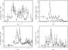 |
Fig. 1 X-ray Chandra (circles) and XMM-Newton PN (squares) X-ray spectra of the Compton-thick AGN candidates PID-66, PID-144 and PID-147 and PID-324. The first and second row give the transmission and reflection dominated AGN, respectively, according to the combined Chandra and XMM-Newton spectral fits. We note the high spectral response of XMM-Newton compared to Chandra at high energies. |
Joint XMM-Newton and Chandra spectral fits to the four more probable Compton-thick sources Power-law + FeKα line (PLCABS+GA) leaving the relative XMM-Newton and Chandra normalization and the energy of the line free.
5.2.2. Reflection model
We fit a reflection model, Magdziarz & Zdziarski (1995) (pexrav + ga in XSPEC notation). The parameters in the PEXRAV model are the Fe abundance, the inclination angle of the reflecting slab, the cut-off energy of the incident power-law and finally the slope of the incident power-law. We found that the first three parameters remain practically unconstrained owing to the large uncertainties. Therefore, we fix the Fe abundance to 1, and the inclination angle of to 45 degrees, while we assume that the incident power-law spectrum has no high energy cut-off (see e.g. Dadina 2008).
For four sources the derived photon index is either very flat (PID-66, Γ = 0.80 ± 0.2) or very steep (PID-222, Γ = 2.95 ± 0.08), (PID-289, Γ = 2.90 ± 0.06), (PID-324,  ). As these values are many σ discrepant with the intrinsic spectral slopes encountered in AGN (see e.g. Nandra & Pounds 1994; Dadina 2008), we choose to fix the photon index to Γ = 1.8. The results are shown again in Table 2.
5.3. More complex spectral models for the four more probable Compton-thick AGN candidates
For the four more probable Compton-thick AGN candidates, we present some additional spectral models for the joint XMM-Newton and Chandra spectral fits. First, we are exploring the exact energy of the FeKα line. This choice is motivated by the results of Iwasawa et al. (2009) who find ionized Fe emission in many Ultra-luminous IRAS galaxies. Moreover, we investigate the effect of leaving the ratio between the Chandra and the XMM-Newton power-law normalization free. We keep the Fe line normalization constant, as this is believed to arise far away from the black hole in type-2 AGN (Shu et al. 2011). Therefore, the present model has two more free parameters, the line energy and the Chandra power-law normalization, which is not tied up to the XMM-Newton power-law normalization (Table 3). We note that the normalization of the Chandra and XMM-Newton power-laws are consistent within the errors (see discussion in Sect. 5.2.1)
A further model contains an additional power-law whose normalization has been set to 3% of the primary power-law. The slope of this power-law has been fixed to the same value as the primary (transmitted) power-law. This component models the scattered (unabsorbed) component along the line of sight which is often detected in type-2 AGN (e.g. Turner et al. 1997). In this model the energy of the FeKα line is left again as a free parameter. The same holds for the normalization of the Chandra power-law which is not tied to the XMM-Newton normalization. The results are presented in Table 4. The spectral fits are, in general, consistent with the simple power-law plus FeKα line fits. The exception is source 66 where the photon-index becomes flatter at the expense of a lower column density. In this case, because of the flatter power-law, the EW becomes higher reaching a value of 1 keV in the case of Chandra . In good agreement with the power-law model presented in Sect. 5.2.1, the four sources (PID-66, 144, 147 and 324) present FeKα line EW higher than ~0.4 keV corroborating their classification as probable Compton-thick candidates.
Joint XMM-Newton and Chandra spectral fits to the four more probable Compton-thick candidates, using a power-law + FeKα line + scattered emission model (PLCABS+GA+PO), leaving the relative XMM-Newton and Chandra normalization and the central energy of the line free.
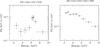 |
Fig. 2 Co-added (rest-frame) X-ray spectra for two sets of sources. Left panel: the four more probable Compton-thick AGN candidates (see text). Right panel: the remaining five sources. |
6. Co-added X-ray spectra
Although there are at least four sources with large FeKα line EW, it is possible that some of the remaining sources have large EW which fail detection owing to the limited photon statistics. In order to answer this question, we derive the co-added X-ray spectrum. The objective is to detect faint FeKα emission that cannot readily be detected in a single source (e.g. Iwasawa et al. 2012b). The data stacking is a straight sum of the rest-frame spectra of individual sources. The individual spectra are binned so that they have a 2–10 keV rest-frame energy range with 200 eV channel width. The data, after background subtraction, are corrected for an efficiency curve determined by the response matrix and auxilliary response file. Finally, each energy bin is corrected for redshift.
In Fig. 2, we present the co-added rest-frame X-ray spectra for two groups of sources. The first group includes the four more probable Compton-thick AGN candidates (PID-66, 144, 147, and 324). The second group includes the remaining sources (PID-48, 214, 222, 245, and 289). A difficulty with the second group is that two of the redshifts (PID-214 and 245) are based on the X-ray spectra and so may be more ambiguous. The first group of sources displays a very prominent FeKα line at a rest-frame energy of 6.4 keV. The second group possibly shows an emission feature but at a higher energy of about 7 keV. If confirmed, this could imply the presence of an ionized FeKα line.
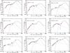 |
Fig. 3 Spectral energy distributions of the nine possible Compton-thick candidates. The red (dot), blue (short dash), and green (long dash) lines denote the stellar, torus, and starburst component, respectively, while the black line denotes the sum of the three components. |
7. Infrared properties
7.1. Spectral energy distributions
We construct spectral energy distributions (SED) for the full sample of our flat spectrum sources, to constrain the predominant powering mechanism (AGN or star formation) in the mid/far IR part of the spectrum. The SEDs are also used to obtain an accurate estimate of the 12 μm nuclear infrared luminosities and thus the X-ray to mid-IR luminosity ratios which are often considered good diagnostics for heavily obscured sources.
We use data from UV wavelengths to the far-IR (where available). Four out of nine sources do not have a far-IR measurement available from Herschel. The data have been modelled using the code originally developed by Fritz et al. (2006). The code has been updated by Feltre et al. (2012). The SED fitting is based on a multicomponent analysis (e.g. Vignali et al. 2009; Hatziminaoglou et al. 2009; Pozzi et al. 2012). The observed UV to far-IR SED is de-composed into three distinct components: a) stars, having the bulk of the emission in the optical/near-IR b) hot dust, mainly heated by UV/optical emission caused by gas accreting onto the supermassive black hole c) colder dust heated by star formation. The stellar component has been included using a set of simple stellar population (SSP) spectra of solar metallicity and ages ranging from ≈1 Myr to ≈8 Gyr. A common value of extinction is applied to stars of all ages, and a Calzetti et al. (2009) attenuation law has been adopted (RV = 4.05). To model the emission at observed wavelengths greater than 24 μm, the SED fitting also includes a component from colder, diffuse dust, most likely heated by start formation processes, as discussed below. This is represented by templates of known starburst galaxies (Vignali et al. 2009). The SED fits are shown in Fig. 3. The four more probable Compton-thick candidates appear to have star-forming components. However, the strength of the star-forming component in PID-66 and PID-147 is ambiguous because of the lack of far-IR data in these sources. The use of templates of nearby starbursts to model the far-IR emission and hence star-formation rates, may present some limitations because there may be discrepancies between typical IR SEDs at high redshift compared to local sources (e.g. Elbaz et al. 2011; Nordon et al. 2012).
Next, we derive the exact star-formation rates and specific star-formation rates, i.e. the ratio of star-formation over the stellar mass. The far-IR luminosity is probably the most reliable tracer of star-forming activity (Kennicutt & Evans 2012). The IR photons are emitted by the dust surrounding young stars, which is heated by their ultra-violet radiation. The star-formation rate is derived from the total IR luminosity (8 − 1000 μm) which is ascribed to star-formation according to the SED decomposition. We use the relation between the IR luminosity and SFR in Murphy et al. (2011): ![\begin{equation} \rm {\it SFR} [{\it M}_\odot\, yr^{-1}] = 3.88 \times 10^{-44} {\it L}(8{-}1000~ \mu m) [erg \,s^{-1}]. \end{equation}](/articles/aa/full_html/2013/07/aa20828-12/aa20828-12-eq194.png) (1)Then, the specific star-formation rate, sSFR, is given by
(1)Then, the specific star-formation rate, sSFR, is given by ![\begin{equation} \rm logs\,{\it SFR} [Gyr^{-1}]=\log {\it SFR} [{\it M}_\odot\, yr^{-1}] - log\, {\it M}^{\star} [{\it M}_\odot] + 8.77. \end{equation}](/articles/aa/full_html/2013/07/aa20828-12/aa20828-12-eq195.png) (2)The stellar mass M⋆ is estimated from the optical part of the SED (for details see Rovilos et al. 2012). Table 5 summarises the IR luminosities, star-formation rate and stellar masses for the heavily obscured AGN in our sample. The typical errors on the 12 μm are about 20% apart from PID-48, PID-66, PID-222, and PID-245 where the uncertainties can be as high as a factor of two. In most cases, the typical errors on the total IR luminosity are between 10 and 20%. In the cases where no far-IR data are available, the errors become large (factors of 2–3). Finally, for the stellar masses the errors are of the order of 10%.
(2)The stellar mass M⋆ is estimated from the optical part of the SED (for details see Rovilos et al. 2012). Table 5 summarises the IR luminosities, star-formation rate and stellar masses for the heavily obscured AGN in our sample. The typical errors on the 12 μm are about 20% apart from PID-48, PID-66, PID-222, and PID-245 where the uncertainties can be as high as a factor of two. In most cases, the typical errors on the total IR luminosity are between 10 and 20%. In the cases where no far-IR data are available, the errors become large (factors of 2–3). Finally, for the stellar masses the errors are of the order of 10%.
Infrared properties of heavily obscured sources.
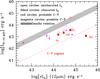 |
Fig. 4 Absorbed X-ray (2–10 keV) X-ray luminosity against the 12 μm luminosity. The large circles correspond to the best candidate Compton-thick sources as suggested by the large equivalent-width FeKα lines. The typical errors are of the order of 30% and 20% for the IR and X-ray luminosity respectively, including the uncertainties in the model fitting. The hatched diagram represents the 1σ envelope of the local (Gandhi et al. 2009) relation. Open circles correspond to X-ray luminosities corrected for absorption (see Table 1). For two sources (PID-222 and PID-324) the absorbed luminosity equals the unabsorbed luminosity. The dotted line corresponds to a factor of 30 lower X-ray luminosity as is typical in many Compton-thick nuclei. |
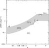 |
Fig. 5 Specific star-formation rate as a function of redshift for eight of the candidate Compton-thick sources. The shaded area gives the star-formation main-sequence according to Elbaz et al. (2010). Above and below this area lie the starburst and quiescent galaxies respectively. Source 222 is not ploted as there is no available rest-frame photometry above a rest-frame wavelength 24 μm. |
7.2. X-ray to IR luminosity ratios
The detection of a low X-ray to mid-IR luminosity ratio has been widely used as the main instrument for the detection of faint Compton-thick AGN which cannot be easily identified in X-ray wavelengths (e.g. Goulding et al. 2011). This is because the mid-IR luminosity (e.g. 12 μm or 6 μm) is a good proxy of the AGN power, as it should be dominated by very hot dust which is heated by the AGN (e.g. Lutz et al. 2004; Maiolino et al. 2007). At these wavelengths the contribution by the stellar-light and colder dust heated by young stars should be small. Gandhi et al. (2009) present high angular resolution mid-IR (12 μm) observations of the nuclei of 42 nearby Seyfert galaxies. These observations provide the least contaminated core fluxes of AGN. These authors find a tight correlation between the near-IR fluxes and the intrinsic X-ray luminosity. Although the Spitzer observations do not have the spatial resolution to resolve the core, the SED decomposition allows us to derive with reasonable accuracy the nuclear IR luminosity. In Fig. 4, we present the obscured X-ray luminosities against the 12 μm luminosities. All four candidate Compton-thick sources have low LX/L12 ratios. Therefore, it appears that the use of the (obscured) X-ray to mid-IR (12 μm) ratio is a reliable diagnostic for the presence of heavily obscured sources. We note that the unobscured X-ray luminosity of at least two sources lies below the Gandhi et al. (2009) relation. This may suggest that these are Compton-thick despite the absence of high-EW FeKα lines.
7.3. Star formation
It has been suggested that highly obscured AGN at X-ray wavelengths may be associated with high rates of star formation (see for example Georgakakis et al. 2003; Rovilos et al. 2007; Mainieri et al. 2011). Alexander et al. (2005) find that many sub-mm galaxies, which have very high rates of star-formation, are associated with heavily absorbed sources in X-ray wavelengths. A possible explanation for such a link would be that the nuclear star-forming region is associated with the X-ray absorbing screen. In Fig. 3, it appears that in the four more probable Compton-thick candidates, the rest-frame mid-IR wavelengths (around 6 μm) are dominated by the torus emission. Only two of the four probable Compton-thick candidates have long-wavelength data (PID-144, PID-324), and the star-forming component is dominated in both cases. In Fig. 5 we plot the specific star-formation rate as a function of redshift. The four candidate Compton-thick sources have a specific star-formation which roughly follows the main star-forming sequence as described by Elbaz et al. (2010). Moreover, it appears that the star-formation properties of the Compton-thick AGN are not different from those of X-ray selected AGN in general (see e.g. Mullaney et al. 2011; Santini et al. 2012; Rosario et al. 2012; Rovilos et al. 2012). Therefore, it appears that there is no link between the presence of a Compton-thick nucleus and enhanced star-formation activity in our sample.
8. Discussion
8.1. Limitations in the sample selection and completeness
We compiled a sample of candidate Compton-thick AGN searching for either flat spectrum sources, i.e. those with Γ < 1.4 (at the 90% confidence level) which is suggestive of a reflection dominated spectrum (e.g. George & Fabian 1991) or those showing an absorption turnover suggesting a rest-frame column density of >1024 cm-2. The deep flux limits of the present observations facilitates the detection of Compton-thick sources. This is because Compton-thick AGN are difficult to detect because they are very faint in the X-rays for the same intrinsic luminosity, meaning that many Compton-thick sources at a given luminosity will be missed because of the effective survey flux limits.
We find nine possible sources among the 176 XMM-Newton spectra examined. Out of these, four show FeKα lines with large equivalent-widths and so these have a higher probability of being Compton-thick. Our sample is by no means complete. For example, at faint fluxes there may be sources which have flat spectra, albeit with larger error bars on Γ and hence fail our selection criterion. Incompleteness may also be introduced by the errors in uncertain redshifts. This is important in the cases where the Compton-thick classification is based on the detection of an absorption turnover.
Next, we discuss whether there are apparently flat X-ray spectrum sources which are not genuinely reflection dominated Compton-thick sources. Most AGN have a steep power-law photon index with a slope of Γ ~ 1.8 and a dispersion of σ = 0.15 (e.g. Nandra & Pounds 1994). Sources which have a significantly flatter photon-index have a high probability of being Compton-thick. However, there are flat-spectrum sources which are probably not Compton-thick. This is because there is a degeneracy between the photon-index and the column density and therefore a moderate column density or a complex/multiple absorber can be mistaken as a flat photon index. For example, in Table 1, we see that source PID-66 (z = 1.185) shows a photon-index of  and
and  cm-2 (3015/2498) when both the photon-index and the column density are left free. When the photon-index is fixed to the more realistic value of Γ = 1.8, the implied column density becomes
  cm-2, while the difference in the Cash statistic (3018/2500) is not statistically significant. This degeneracy can be seen even in sources with large numbers of photon counts. Corral et al. (2011) present an X-ray spectral analysis of ~300 AGN from the XMM-Newton bright survey. There are several sources (e.g. XBSJ134656.7+580315 at a redshift of z = 0.373), at bright fluxes (f2 − 10 > 10-13 erg cm-2 s-1) and hence with excellent photon statistics which present a flat power-law as the best-fit. Corral et al. (2011) point out that there are no iron lines with large EW detected in these sources. If the photon-index is fixed at Γ = 1.9 the resulting column density is of the order ~ 1023 cm-2 and therefore these sources, although certainly heavily obscured, are not Compton-thick.
8.2. The X-ray spectrum of Compton-thick AGN
Additional ambiguities in the selection may be introduced by uncertainties in the X-ray spectrum of Compton-thick AGN. Brightman & Ueda (2012) perform a selection of Compton-thick sources among the Chandra sources in the 4 Ms CDF-S data using their own spectral models. These take into account Compton-scattering, the geometry of the circumnuclear matter, and the scattered nuclear light. The amount of scattered light decreases with increasing column density. They find two sources with a large scattering component (>5%) and hence steeper spectra. These amounts of scattered light are well above those detected in local Compton-thick AGN (e.g. Comastri et al. 2010). Evidently, Compton-thick sources with steep spectra would have avoided detection in our selection criterion.
The strength of the FeKα line introduces an additional uncertainty. The presence of an FeKα line with a large EW is considered to be the “smoking gun” for the presence of a Compton-thick nucleus. Comastri et al. (2010) present Suzaku observations of a few Compton-thick sources. They find narrow FeKα lines (EW ~ 1–2 keV) due to neutral or mildly ionized gas in all of them. Fukazawa et al. (2011) present Suzaku observations of a sample of nearby Seyfert galaxies among which many are Compton-thick. They find that all Compton-thick sources present FeKα lines with an EW exceeding 0.5 keV. However, there have been rare examples of Compton-thick sources with small EW. One of these examples is the Broad-absorption-Line QSO Mrk231. Its BeppoSAX spectrum (Braito et al. 2004) shows that it is Compton-thick (with a column density of ~ 1024 cm-2), but it has an FeKα line with an EW of only 0.3 keV. Moreover, recent Suzaku observations showed a decrease in the covering fraction of the absorber (Piconcelli et al. 2013).
8.3. Previous studies of heavily obscured AGN in the CDF-S
Tozzi et al. (2006) first derived a sample of candidate Compton-thick sources in the 1 Ms CDF-S observations based on X-ray spectral fits. They derived a sample of 20 candidate Compton-thick sources. Georgantopoulos et al. (2007) performed the same exercise compiling a sample of 18 sources in the same dataset but using slightly different spectral models. Only nine of the sources are common in these two samples, demonstrating that the uncertainties in this technique are considerable. From the Compton-thick candidates in Tozzi et al. (2006) or Georgantopoulos et al. (2007), only two sources are found in our present XMM-Newton sample.
Comastri et al. (2011) used the 3 Ms XMM-Newton data in the CDF-S attempting to confirm that some of the Compton-thick candidates in the above samples are most probably Compton-thick AGN. The excellent quality XMM-Newton data and in particular its ability to detect the FeKα line allowed the above authors to confirm the best two examples of Compton-thick candidates in the high redshift Universe, PID-144 and PID-147 at redshifts of z = 1.53 and z = 3.7 respectively. We note that PID-144 was first reported as Compton-thick by Norman et al. (2002) on the basis of 1 Ms Chandra spectroscopy.
For PID-144, Comastri et al. (2011) fit an absorbed power-law model finding a photon-index of  with a column density of
  cm-2 i.e. favouring a transmission-dominated heavily obscured source. Moreover, they detect a strong FeKα line with an EW of
  eV. Our joint XMM-Newton /Chandra spectral fit (Table 2) suggests a transmission-dominated highly obscured spectrum with
  cm-2 and a photon index of
  fully consistent with the results of Comastri et al. (2011). The FeKα line EW is somewhat lower (
 eV) but fully consistent with the above results.
In the case of PID-147, Comastri et al. (2011) find that a good fit to the data is provided by an absorbed power-law model with a column density of  cm-2 and a photon index of Γ = − 0.11 ± 0.22; the iron line has a very large EW (
 eV). Our combined XMM-Newton and Chandra spectral fits (Table 2) give a higher column density of
  cm-2 but with a steeper photon-index
  , from which a smaller equivalent width (
 eV). Further exploration of the spectra suggests that the difference can be ascribed to degeneracies in the parameter space, coupled with the different treatment of statistic (c-stat vs. χ2) and binning of the spectra, which may result in different local minima for the statistic parameter.
Brightman & Ueda (2012) report 20 Compton-thick AGN. Out of these, five have been reported as Compton-thick in Tozzi et al. (2006) while three in Georgantopoulos et al. (2007). The two Compton-thick sources reported by Comastri et al. (2011) (144 and 147) and in our paper have column densities just below 1024 cm-2 in the spectral fits of Brightman & Ueda (2012). Recently, Iwasawa et al. (2012a) have performed a search for heavily obscured AGN in the same XMM-Newton sample as the one presented here. They are using an X-ray colour-colour diagram based on the rest-frame 3–5 keV, 5–9 keV, and 9–20 keV bands. They find a sample of seven candidate heavily obscured sources at high-redshift (z > 1.7) having rest-frame 9–20 keV excess emission. Some of them are good Compton-thick candidates either on the basis of a high-EW (>1 keV) FeKα line (e.g. PID-114 at z = 1.806) or directly on the basis of large column densities (NH ≈ 1024 cm-2) (PID-245, 252).
8.4. Comparison with X-ray background synthesis models
We compare the number of Compton-thick AGN found here with the predictions of X-ray background synthesis models (e.g. Gilli et al. 2007; Treister et al. 2009a; Ballantyne et al. 2011; Akylas et al. 2012) In our sample, we find four probable candidate Compton-thick sources two of which appear to be transmission-dominated. Comparing with the models of Gilli et al. (2007)2, we find that the number of Compton-thick sources is ≈7 in our field down to the flux limit of the present survey f(2 − 10) ~ 1 × 10-15 erg cm-2 s-1. The model of Treister et al. (2009a)3 predicts a number of 8 Compton-thick in the same area. Finally, the model of Akylas et al. (2012)4 yields about 11 Compton-thick sources in our field. All the above estimates refer only to transmission dominated (log NH = 24 − 25) Compton-thick AGN. If we include the reflection-dominated AGN (log NH = 25 − 26) in the model of Gilli et al. (2007), the total number of Compton-thick AGN rises to ≈11. Interestingly, the model of Akylas et al. (2012) has a lower intrinsic fraction of Compton-thick AGN compared to that of Gilli et al. (2007), 15% compared to 33%. However, the higher number of Compton-thick AGN predicted by Akylas et al. (2012) at the relatively bright fluxes probed here, is a consequence of the stronger reflection component predicted by this model. The fact that the number of the Compton-thick candidates found here is systematically lower than those predicted by all X-ray background synthesis models may suggest that our sample suffers from incompleteness.
8.5. Concluding remarks
The selection of Compton-thick AGN on the basis of either an absorption turnover (transmission dominated) or a flat spectrum (reflection dominated) appears to be sufficiently robust. The presence of a high EW FeKα line can be considered as the final diagnostic for the presence of a Compton-thick AGN despite some possible exceptions mentioned above (e.g. Mrk 231). On the basis of the above diagnostic, we isolate four sources as excellent candidates for being Compton-thick. These are probably the best Compton-thick candidates at moderate to high redshifts found so far. Still, the number found here is a factor of at least two lower compared to the predictions of X-ray background synthesis models. This may imply that a number of Compton-thick AGN (particularly those at the faintest fluxes) fail to be classified as Compton-thick. It is likely that these lie among our remaining five flat spectrum sources. Then we did not classify them securely as Compton-thick because we failed to detect strong EW FeKα lines. The fact that a few sources lie below the Gandhi et al. (2009) unabsorbed X-ray-to-IR luminosity relation may point towards this scenario. This stresses the need for complementary IR methods together with X-ray spectroscopy, to better understand the properties of Compton-thick AGN.
9. Summary
We report on an X-ray spectral study of the 176 brightest sources in the XMM-Newton survey in the CDF-S. The aim is to identify very highly obscured (Compton-thick) AGN. Our methodology consists of looking for sources which have either an absorption cut-off characteristic of a high column density or a flat spectrum (the 90% upper limit of the photon index should be lower than 1.4). After the selection of our candidate sources, we are also looking for the presence of a strong FeKα line which is considered to be the trademark of a highly obscured source. Our results can be briefly summarised as follows:
-
The XMM-Newton spectra select nineCompton-thick candidates. We separate a group of four sourceswhich have large iron line EW and, therefore, these have higherprobability of being Compton-thick. Adding theChandra data to the spectral fits corroborates ourprevious results. Two of the sources are most likely transmissiondominated (PID-66 and PID-144), while the other two arereflection dominated (PID-147 and PID-324).
-
Although our sample is by no means statistically complete, it represents the examples of Compton-thick AGN at moderate to high redshifts. In particular, the redshifts of the four most probable candidate Compton-thick sources are z = 1.185, 1.222, 1.53 and 3.7. One of our probable Compton-thick candidates (PID-66) is presented here for the first time. The XMM-Newton spectra of two sources (PID-144 and PID-147) have been reported in Comastri et al. (2011) while their combined XMM/Chandra spectrum is presented here for the first time. Finally, one source (PID-324) has been reported in detail in Georgantopoulos et al. (2011a).
-
The X-ray-to-mid-IR (12 μm) luminosity ratio of the four more probable Compton-thick candidates are well below the average relation of Gandhi et al. (2009), independently suggesting heavy obscuration.
-
Spitzer and Herschel observations of our four candidate Compton-thick sources derive star-formation rates between about 25 and 1000 M⊙ yr-1. Their specific star-formation rates are consistent with those of normal galaxies suggesting that heavy obscuration is not related to enhanced star-formation.
Acknowledgments
I.G. and A.C. acknowledge the Marie Curie fellowship FP7-PEOPLE-IEF-2008 Prop. 235285. We acknowledge financial contribution from the agreement ASI-INAF I/009/10/0. P.R. acknowledges the receipt of a fellowship (proposal no. P9-3493) from the Greek Secretariat of Research and Technology in the framework of the project “Support to postdoctoral researchers”. N.C. acknowledges financial support from the Della Riccia foundation. F.J.C. acknowledges partial financial support by the Spanish Ministry of Economy and Competitiveness through the grant AYA2010-21490-C02-01. The Chandra data used were taken from the Chandra Data Archive at the Chandra X-ray Center.
References
- Ajello, M., Rau, A., Greiner, J., et al. 2008, ApJ, 673, 96 [NASA ADS] [CrossRef] [Google Scholar]
- Akylas, A., & Georgantopoulos, I. 2009, A&A, 500, 999 [NASA ADS] [CrossRef] [EDP Sciences] [Google Scholar]
- Akylas, A., Georgakakis, A., Georgantopoulos, I., Brightman, M., & Nandra, K., 2012, A&A, 546, A98 [NASA ADS] [CrossRef] [EDP Sciences] [Google Scholar]
- Alexander, D. M., Bauer, F. E., Brandt, W. N., et al. 2003, AJ, 126, 539 [NASA ADS] [CrossRef] [Google Scholar]
- Alexander, D. M., Bauer, F. E., Chapman, S. C., et al. 2005, ApJ, 632, 736 [NASA ADS] [CrossRef] [Google Scholar]
- Alexander, D. M., Chary, R. R., Pope, A., et al. 2008, ApJ, 687, 835 [NASA ADS] [CrossRef] [Google Scholar]
- Alexander, D. M., Bauer, F. E., Brandt, W. N., et al. 2011, ApJ, 738, 44 [NASA ADS] [CrossRef] [Google Scholar]
- Arnaud, K. A. 1996, Astronomical Data Analysis Software and Systems V, eds. G. Jacoby, & J. Barnes, ASP Conf. Ser., 101, 17 [Google Scholar]
- Balestra, I., Mainieri, V., Popesso, P., et al. 2010, A&A, 512, A12 [NASA ADS] [CrossRef] [EDP Sciences] [Google Scholar]
- Ballantyne, D. R., Draper, A. R., Madsen, K. K., Rigby, J. R., & Treister, E., 2011, ApJ, 736, 56 [NASA ADS] [CrossRef] [Google Scholar]
- Barger, A., Cowie, L., Capak, P., et al. 2003, AJ, 126, 632 [NASA ADS] [CrossRef] [Google Scholar]
- Braito, V., Della Ceca, R., Piconcelli, E., et al. 2004, A&A, 420, 79 [NASA ADS] [CrossRef] [EDP Sciences] [Google Scholar]
- Brandt, W. N., & Hasinger, G. 2005, ARA&A, 43, 827 [Google Scholar]
- Brightman, M., & Nandra, K. 2011, MNRAS, 413, 1206 [CrossRef] [Google Scholar]
- Brightman, M., & Ueda, Y. 2012, MNRAS, 423, 702 [NASA ADS] [CrossRef] [Google Scholar]
- Burlon, D., Ajello, M., Greiner, J., et al. 2011, ApJ, 728, 58 [NASA ADS] [CrossRef] [Google Scholar]
- Calzetti, D. 2009, ASPC, 414, 214 [NASA ADS] [Google Scholar]
- Cardamone, C. N., van Dokkum, P. G., Urry, C. M., et al. 2010, ApJS, 189, 270 [NASA ADS] [CrossRef] [Google Scholar]
- Cash, W. 1979, ApJ, 228, 939 [NASA ADS] [CrossRef] [Google Scholar]
- Churazov, E., Sunyaev, R., Revnivtsev, M., et al. 2007, A&A, 467, 529 [NASA ADS] [CrossRef] [EDP Sciences] [Google Scholar]
- Comastri, A. 2004, ASSL, 308, 245 [Google Scholar]
- Comastri, A., Iwasawa, K., Gilli, R., et al. 2010, ApJ, 717, 787 [NASA ADS] [CrossRef] [Google Scholar]
- Comastri, A., Ranalli, P., Iwasawa, K., et al. 2011, A&A, 526, L9 [NASA ADS] [CrossRef] [EDP Sciences] [Google Scholar]
- Cooper, M. C., Yan, R., Dickinson, M., et al. 2012, MNRAS, 425, 2116 [NASA ADS] [CrossRef] [Google Scholar]
- Corral, A., Della Ceca, R., Caccianiga, A., et al. 2011, A&A, 530, A42 [NASA ADS] [CrossRef] [EDP Sciences] [Google Scholar]
- Daddi, E., Alexander, D. M., Dickinson, M., et al. 2007, ApJ, 670, 173 [NASA ADS] [CrossRef] [Google Scholar]
- Dadina, M. 2008, A&A, 485, 417 [NASA ADS] [CrossRef] [EDP Sciences] [Google Scholar]
- Dahlen, T., Mobasher, B., Dickinson, M., et al. 2010, ApJ, 724, 425 [NASA ADS] [CrossRef] [Google Scholar]
- Damen, M., Labbé, I., van Dokkum, P. G., et al. 2011, ApJ, 727, 1 [NASA ADS] [CrossRef] [Google Scholar]
- Dickey, J. M., & Lockman, F. J. 1990, ARA&A, 28, 215 [NASA ADS] [CrossRef] [MathSciNet] [Google Scholar]
- Eckart, M. E., McGreer, I. D., Stern, D., Harrison, F. A., & Helfand, D. J. 2010, ApJ, 708, 584 [NASA ADS] [CrossRef] [Google Scholar]
- Elbaz, D., Hwang, H. S., Magnelli, B., et al. 2010, A&A, 518, L29 [NASA ADS] [CrossRef] [EDP Sciences] [Google Scholar]
- Elbaz, D., Dickinson, M., Hwang, H. S., et al. 2011, A&A, 533, A119 [NASA ADS] [CrossRef] [EDP Sciences] [Google Scholar]
- Feltre, A., Hatziminaoglou, E., Fritz, J., & Franceschini 2012, MNRAS, 426, 120 [NASA ADS] [CrossRef] [Google Scholar]
- Feruglio, C., Daddi, E., Fiore, F., et al. 2011, ApJ, 729, L4 [NASA ADS] [CrossRef] [Google Scholar]
- Fiore, F., Grazian, A., Santini, P., et al. 2008, ApJ, 672, 94 [NASA ADS] [CrossRef] [Google Scholar]
- Fiore, F., Puccetti, S., Brusa, M., et al. 2009, ApJ, 693, 447 [NASA ADS] [CrossRef] [Google Scholar]
- Fritz, J., Franceschini, A., & Hatziminaoglou, E. 2006, MNRAS, 366, 767 [Google Scholar]
- Frontera, F., Orlandini, M., & Landi, R. 2007, ApJ, 666, 86 [NASA ADS] [CrossRef] [Google Scholar]
- Fukazawa, Y., Hiragi, K., Mizuno, M., et al. 2011, ApJ, 727, 19 [NASA ADS] [CrossRef] [Google Scholar]
- Gandhi, P., Horst, H., Smette, A., et al. 2009, A&A, 502, 457 [NASA ADS] [CrossRef] [EDP Sciences] [Google Scholar]
- Georgakakis, A., Hopkins, A. M., Sullivan, M., et al. 2003, MNRAS, 345, 939 [NASA ADS] [CrossRef] [Google Scholar]
- Georgantopoulos, I. 2012 [arXiv:1204.2173] [Google Scholar]
- Georgantopoulos, I., Georgakakis, A., & Akylas, A. 2007, A&A, 466, 823 [NASA ADS] [CrossRef] [EDP Sciences] [Google Scholar]
- Georgantopoulos, I., Georgakakis, A., Rowan-Robinson, M., & Rovilos, E. 2008, A&A, 484, 671 [NASA ADS] [CrossRef] [EDP Sciences] [Google Scholar]
- Georgantopoulos, I., Akylas, A., Georgakakis, A., & Rowan-Robinson, M. 2009, A&A, 507, 747 [NASA ADS] [CrossRef] [EDP Sciences] [Google Scholar]
- Georgantopoulos, I., Dasyra, K., Rovilos, E., et al. 2011a, A&A, 531, A116 [NASA ADS] [CrossRef] [EDP Sciences] [Google Scholar]
- Georgantopoulos, I., Rovilos, E., Xilouris, E. M., Comastri, A., & Akylas, A. 2011b, A&A, 526, A86 [NASA ADS] [CrossRef] [EDP Sciences] [Google Scholar]
- George, I., & Fabian, A. C. 1991, MNRAS, 249, 352 [NASA ADS] [CrossRef] [Google Scholar]
- Giacconi, R., Gursky, H., Paolini, F. R., & Rossi, B. B. 1962, Phys. Rev. Lett., 9, 439 [NASA ADS] [CrossRef] [Google Scholar]
- Giacconi, R., Zirm, A., Wang, J., et al. 2002, ApJS, 139, 369 [NASA ADS] [CrossRef] [Google Scholar]
- Gilli, R., Comastri, A., & Hasinger, G. 2007, A&A, 463, 79 [NASA ADS] [CrossRef] [EDP Sciences] [Google Scholar]
- Gilli, R., Vignali, C., Mignoli, M., et al. 2010, A&A, 519, A92 [NASA ADS] [CrossRef] [EDP Sciences] [Google Scholar]
- Gilli, R., Su, J., Norman, C., et al. 2011, ApJ, 730, L28 [NASA ADS] [CrossRef] [Google Scholar]
- Goulding, A. D., Alexander, D. M., Mullaney, J. R., et al. 2011, MNRAS, 411, 1231 [NASA ADS] [CrossRef] [Google Scholar]
- Goulding, A. D., Alexander, D. M., Bauer, F. E., et al. 2012, ApJ, 755, 5 [Google Scholar]
- Hatziminaoglou, E., Fritz, J., & Jarrett, T. H. 2009, MNRAS, 399, 1206 [NASA ADS] [CrossRef] [Google Scholar]
- Iwasawa, K., Crawford, C. S., Fabian, A. C., & Wilman, R. J. 2005, MNRAS, 326, L20 [NASA ADS] [CrossRef] [Google Scholar]
- Iwasawa, K., Sanders, D. B., Evans, A. S., et al. 2009, ApJ, 695, L103 [NASA ADS] [CrossRef] [Google Scholar]
- Iwasawa, K., Gilli, R., Vignali, C., et al. 2012a, A&A, 546, A84 [NASA ADS] [CrossRef] [EDP Sciences] [Google Scholar]
- Iwasawa, K., Mainieri, V., Brusa, M., et al. 2012b, A&A, 537, A86 [NASA ADS] [CrossRef] [EDP Sciences] [Google Scholar]
- Kennicutt, R. C., & Evans, N.J., 2012, ARA&A, 50, 531 [NASA ADS] [CrossRef] [Google Scholar]
- Le Fèvre, O., Vettolani, G., Garilli, B., et al. 2005, A&A, 439, 845 [NASA ADS] [CrossRef] [EDP Sciences] [Google Scholar]
- Lehmer, B. D., Brandt, W. N., Alexander, D. M., et al. 2005, ApJS, 161, 21 [NASA ADS] [CrossRef] [Google Scholar]
- Luo, B., Bauer, F. E., Brandt, W. N., et al. 2008, ApJS, 179, 19 [NASA ADS] [CrossRef] [Google Scholar]
- Luo, B., Brandt, W. N., Xue, Y. Q., et al. 2010, ApJS, 187, 560 [NASA ADS] [CrossRef] [Google Scholar]
- Lutz, D., Maiolino, R., Spoon, H. W. W., & Moorwood, A. F. M. 2004, A&A, 418, 465 [NASA ADS] [CrossRef] [EDP Sciences] [Google Scholar]
- Magdziarz, P. A., & Zdziarski, A. 1995, MNRAS, 273, 837 [NASA ADS] [CrossRef] [Google Scholar]
- Magnelli, B., Elbaz, D., Chary, R. R., et al. 2009, A&A, 496, 57 [NASA ADS] [CrossRef] [EDP Sciences] [Google Scholar]
- Mainieri, V., Bongiorno, A., Merloni, A., et al. 2011, A&A, 535, A80 [NASA ADS] [CrossRef] [EDP Sciences] [Google Scholar]
- Maiolino, R., Shemmer, O., Imanishi, M., et al. 2007, A&A, 468, 979 [NASA ADS] [CrossRef] [EDP Sciences] [Google Scholar]
- Malizia, A., Bassani, L., Bazzano, A., et al. 2012, MNRAS, 426, 1750 [NASA ADS] [CrossRef] [Google Scholar]
- Marconi, A., Risaliti, G., Gilli, R., et al. 2004, MNRAS, 351, 169 [NASA ADS] [CrossRef] [Google Scholar]
- Matt, G., Bianchi, S., Guainazzi, M., & Molendi, S. 2004, A&A, 414, 155 [NASA ADS] [CrossRef] [EDP Sciences] [Google Scholar]
- Merloni, A., & Heinz, S. 2008, MNRAS, 388, 1011 [NASA ADS] [Google Scholar]
- Moretti, A., Pagani, C., Cusumano, G., et al. 2009, A&A, 493, 501 [NASA ADS] [CrossRef] [EDP Sciences] [Google Scholar]
- Moretti, A., Vattakunnel, S., Tozzi, P., et al. 2012, A&A, 548, A87 [NASA ADS] [CrossRef] [EDP Sciences] [Google Scholar]
- Mullaney, J. R., Alexander, D. M., Goulding, A. D., & Hickox, R. C. 2011, MNRAS, 414, 1082 [NASA ADS] [CrossRef] [Google Scholar]
- Murphy, E. J., Condon, J. J., & Schinnerer, E. 2011, ApJ, 737, 67 [NASA ADS] [CrossRef] [Google Scholar]
- Nandra, K., & Pounds, K. A., 1994, MNRAS, 268, 405 [NASA ADS] [CrossRef] [Google Scholar]
- Nordon, R., Lutz, D., Genzel, R., et al. 2012, A&A, 745, A182 [Google Scholar]
- Norman, C., Hasinger, G., Giacconi, R., et al. 2002, ApJ, 571, 218 [NASA ADS] [CrossRef] [Google Scholar]
- Norris, R. P., Afonso, J., Appleton, P. N., et al. 2006, AJ, 132, 2409 [NASA ADS] [CrossRef] [Google Scholar]
- Oliver, S., Bock, J., Altieri, B., et al. 2012, MNRAS, 424, 1614 [NASA ADS] [CrossRef] [EDP Sciences] [Google Scholar]
- Paltani, S., Walter, R., McHardy, I. M., et al. 2008, A&A, 485, 707 [NASA ADS] [CrossRef] [EDP Sciences] [Google Scholar]
- Piconcelli, E., Miniutti, G., Ranalli, P., et al. 2013, MNRAS, 428, 1185 [NASA ADS] [CrossRef] [Google Scholar]
- Pozzi, F., Vignali, C., Gruppioni, C., et al. 2012, MNRAS, 423, 1909 [NASA ADS] [CrossRef] [Google Scholar]
- Rafferty, D. A., Brandt, W. N., Alexander, D. M., et al. 2011, ApJ, 742, 3 [NASA ADS] [CrossRef] [Google Scholar]
- Ranalli, P., Comastri, A., Vignali, C., et al. 2013, A&A, 555, A42 [NASA ADS] [CrossRef] [EDP Sciences] [Google Scholar]
- Ravikumar, C. D., Puech, M., Flores, H., et al. 2007, A&A, 465, 1099 [NASA ADS] [CrossRef] [EDP Sciences] [Google Scholar]
- Ricci, C., Walter, R., Courvoisier, T. J.-L., & Paltani, S. 2011, A&A, 532, A102 [NASA ADS] [CrossRef] [EDP Sciences] [Google Scholar]
- Rosario, D. J., Santini, P., Lutz, D., et al. 2012, A&A, 545, A45 [NASA ADS] [CrossRef] [EDP Sciences] [Google Scholar]
- Rovilos, E., Georgakakis, A., Georgantopoulos, I., et al. 2007, A&A, 466, 119 [NASA ADS] [CrossRef] [EDP Sciences] [Google Scholar]
- Rovilos, E., Comastri, A., Gilli, R., et al. 2012, A&A, 546, A58 [Google Scholar]
- Santini, P., Fontana, A., Grazian, A., et al. 2009, A&A, 504, 751 [NASA ADS] [CrossRef] [EDP Sciences] [Google Scholar]
- Santini, P., Rosario, D. J., Shao, L., et al. 2012, A&A, 540, A109 [NASA ADS] [CrossRef] [EDP Sciences] [Google Scholar]
- Sazonov, S., Krivonos, R., Revnivtsev, M., Churazov, E., & Sunyaev, R. 2008, A&A, 482, 517 [NASA ADS] [CrossRef] [EDP Sciences] [Google Scholar]
- Silverman, J. D., Mainieri, V., Salvato, M., et al. 2010, ApJS, 191, 124 [NASA ADS] [CrossRef] [Google Scholar]
- Shu, X. W., Yaqoob, T., & Wang, J. X. 2011, ApJ, 738, 147 [NASA ADS] [CrossRef] [Google Scholar]
- Soltan, A. 1982, MNRAS, 200, 115 [NASA ADS] [CrossRef] [Google Scholar]
- Szokoly, G. P., Bergeron, J., Hasinger, G., et al. 2004, ApJS, 155, 271 [NASA ADS] [CrossRef] [Google Scholar]
- Taylor, E. N., Franx, M., van Dokkum, P. G., et al. 2009, ApJS, 183, 295 [NASA ADS] [CrossRef] [Google Scholar]
- Tozzi, P., Gilli, R., Mainieri, V., et al. 2006, A&A, 451, 457 [NASA ADS] [CrossRef] [EDP Sciences] [Google Scholar]
- Treister, E., Urry, C. M., & Virani, S. 2009a, ApJ, 696, 110 [NASA ADS] [CrossRef] [Google Scholar]
- Treister, E., Cardamone, C. N., Schawinski, K., et al. 2009b, ApJ, 706, 535 [NASA ADS] [CrossRef] [Google Scholar]
- Tueller, J., Mushotzky, R. F., Barthelmy, S., et al. 2008, ApJ, 681, 113 [NASA ADS] [CrossRef] [Google Scholar]
- Turner, J. T., George, I. M., Nandra, K., & Mushotzky, R. F. 1997, ApJ, 488, 164 [NASA ADS] [CrossRef] [Google Scholar]
- Vanzella, E., Cristiani, S., Dickinson, M., et al. 2008, A&A, 478, 83 [NASA ADS] [CrossRef] [EDP Sciences] [Google Scholar]
- Vignali, C., Pozzi, F., Fritz, J., et al. 2009, A&A, 395, 2189 [Google Scholar]
- Winter, L. M., Mushotzky, R. F., Reynolds, C. S., & Tueller, J. 2009, ApJ, 690, 1322 [NASA ADS] [CrossRef] [Google Scholar]
- Worsley, M. A., Fabian, A. C., Bauer, F. E., et al. 2005, MNRAS, 357, 1281 [NASA ADS] [CrossRef] [Google Scholar]
- Worsley, M. A., Fabian, A. C., Pooley, G. G., & Chandler, C. J. 2006, MNRAS, 368, 844 [NASA ADS] [CrossRef] [Google Scholar]
- Xue, Y. Q., Luo, B., Brandt, W. N., et al. 2011, ApJS, 195, 10 [NASA ADS] [CrossRef] [Google Scholar]
- Xue, Y. Q., Wang, S. X., Brandt, W. N., et al. 2012, ApJ, 758, 129 [NASA ADS] [CrossRef] [Google Scholar]
- Yaqoob, T. 1997, ApJ, 479, 184 [NASA ADS] [CrossRef] [Google Scholar]
All Tables
Initial selection of Compton-thick candidates based on XMM-Newton absorbed power-law, (PLCABS), spectral fits.
Joint XMM and Chandra spectral fits of the full sample of Compton-thick candidates.
Joint XMM-Newton and Chandra spectral fits to the four more probable Compton-thick sources Power-law + FeKα line (PLCABS+GA) leaving the relative XMM-Newton and Chandra normalization and the energy of the line free.
Joint XMM-Newton and Chandra spectral fits to the four more probable Compton-thick candidates, using a power-law + FeKα line + scattered emission model (PLCABS+GA+PO), leaving the relative XMM-Newton and Chandra normalization and the central energy of the line free.
All Figures
|
Fig. 1 X-ray Chandra (circles) and XMM-Newton PN (squares) X-ray spectra of the Compton-thick AGN candidates PID-66, PID-144 and PID-147 and PID-324. The first and second row give the transmission and reflection dominated AGN, respectively, according to the combined Chandra and XMM-Newton spectral fits. We note the high spectral response of XMM-Newton compared to Chandra at high energies. |
| In the text | |
|
Fig. 2 Co-added (rest-frame) X-ray spectra for two sets of sources. Left panel: the four more probable Compton-thick AGN candidates (see text). Right panel: the remaining five sources. |
| In the text | |
|
Fig. 3 Spectral energy distributions of the nine possible Compton-thick candidates. The red (dot), blue (short dash), and green (long dash) lines denote the stellar, torus, and starburst component, respectively, while the black line denotes the sum of the three components. |
| In the text | |
|
Fig. 4 Absorbed X-ray (2–10 keV) X-ray luminosity against the 12 μm luminosity. The large circles correspond to the best candidate Compton-thick sources as suggested by the large equivalent-width FeKα lines. The typical errors are of the order of 30% and 20% for the IR and X-ray luminosity respectively, including the uncertainties in the model fitting. The hatched diagram represents the 1σ envelope of the local (Gandhi et al. 2009) relation. Open circles correspond to X-ray luminosities corrected for absorption (see Table 1). For two sources (PID-222 and PID-324) the absorbed luminosity equals the unabsorbed luminosity. The dotted line corresponds to a factor of 30 lower X-ray luminosity as is typical in many Compton-thick nuclei. |
| In the text | |
|
Fig. 5 Specific star-formation rate as a function of redshift for eight of the candidate Compton-thick sources. The shaded area gives the star-formation main-sequence according to Elbaz et al. (2010). Above and below this area lie the starburst and quiescent galaxies respectively. Source 222 is not ploted as there is no available rest-frame photometry above a rest-frame wavelength 24 μm. |
| In the text | |
Current usage metrics show cumulative count of Article Views (full-text article views including HTML views, PDF and ePub downloads, according to the available data) and Abstracts Views on Vision4Press platform.
Data correspond to usage on the plateform after 2015. The current usage metrics is available 48-96 hours after online publication and is updated daily on week days.
Initial download of the metrics may take a while.