| Issue |
A&A
Volume 553, May 2013
|
|
|---|---|---|
| Article Number | A94 | |
| Number of page(s) | 6 | |
| Section | Galactic structure, stellar clusters and populations | |
| DOI | https://doi.org/10.1051/0004-6361/201321057 | |
| Published online | 16 May 2013 | |
Research Note
The case for high precision in elemental abundances of stars in the era of large spectroscopic surveys
Lund Observatory, Department of Astronomy and Theoretical Physics, Lund University, Box 43, 22100 Lund, Sweden
e-mail: lennart@astro.lu.se; sofia@astro.lu.se
Received: 8 January 2013
Accepted: 11 April 2013
Context. A number of large spectroscopic surveys of stars in the Milky Way are under way or are being planned. In this context it is important to discuss the extent to which elemental abundances can be used as discriminators between different (known and unknown) stellar populations in the Milky Way.
Aims. We aim to establish the requirements in terms of precision in elemental abundances, as derived from spectroscopic surveys of the Milky Way’s stellar populations, in order to detect interesting substructures in elemental abundance space.
Methods. We used Monte Carlo simulations to examine under which conditions substructures in elemental abundance space can realistically be detected.
Results. We present a simple relation between the minimum number of stars needed to detect a given substructure and the precision of the measurements. The results are in agreement with recent small- and large-scale studies, with high and low precision, respectively.
Conclusions. Large-number statistics cannot fully compensate for low precision in the abundance measurements. Each survey should carefully evaluate what the main science drivers are for the survey and ensure that the chosen observational strategy will result in the precision necessary to answer the questions posed.
Key words: methods: data analysis / methods: statistical / stars: abundances / Galaxy: abundances
© ESO, 2013
1. Introduction
In Galactic archaeology stars are used as time capsules. The outer layers of their atmospheres, accessible to spectroscopic studies, are presumed to keep a fair representation of the mixture of elements present in the gas cloud out of which they formed. By determining the elemental abundances in the stellar photospheres, and combining with kinematics and age information, it is possible to piece together the history of the Milky Way (e.g., Freeman & Bland-Hawthorn 2002).
Edvardsson et al. (1993) were among the first to demonstrate that it is possible to achieve high precision in studies of elemental abundances for large samples of long-lived dwarf stars. In their study of 189 nearby dwarf stars they achieved a precision 1 better than 0.05 dex for many elements, including iron and nickel. More recent studies have achieved similar or even better results. Nissen & Schuster (2010), in a study of dwarf stars in the halo, obtain a precision of 0.02–0.04 dex for α-elements relative to iron, and 0.01 dex for nickel relative to iron. In studies of solar twins (i.e., stars whose stellar parameters, including metallicity, closely match those of the sun) Meléndez et al. (2012) are able to achieve a precision better than 0.01 dex. At the same time several studies have found that in the solar neighbourhood there exist substructures in the elemental abundance trends with differences as large as 0.1 to 0.2 dex (e.g. Fuhrmann 1998; Bensby et al. 2004; Nissen & Schuster 2010).
Driven both by technological advances and the need for ground-based observations to complement and follow up the expected observations from the Gaia satellite, Galactic astronomy is entering a new regime where elemental abundances are derived for very large samples of stars. Dedicated survey telescopes and large surveys using existing telescopes have already moved Galactic astronomy into the era of large spectroscopic surveys (Zwitter et al. 2008; Yanny et al. 2009; Majewski et al. 2010; Gilmore et al. 2012). With the new surveys, several hundred thousands of stars will be observed for each stellar component of the Galaxy. For all of these stars we will have elemental abundances as well as kinematics and, when feasible, ages. One goal for these studies is to quantify the extent to which the differences in elemental abundances seen in the solar neighbourhood extend to other parts of the stellar disk(s) and halo, and to identify other (as yet unknown) components that may exist here and elsewhere.
Large-scale surveys naturally tend to have lower signal-to-noise ratios for the individual stars than can be achieved in the classical studies of small stellar samples in the solar neighbourhood. On the other hand, the very large number of stars reached with the new surveys will at least partly compensate for a lower precision per object. A relevant question is thus: how many stars do we need to detect a certain abundance signature of Y dex, when we have a precision of Z dex in the individual abundance determinations? This is what we explore in this Research Note.
This Research Note is structured as follows: Section 2 sets out the problem which is then investigated in Sect. 3. In Sect. 4 we discuss what accuracies and precisions have been shown to be possible and what is feasible to expect from large scale surveys. Section 5 contains some concluding remarks.
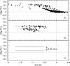 |
Fig. 1 Illustration of the problem, showing Fe and Mg abundances for stars in the solar neighbourhood. a) Based on data by Fuhrmann (see text for references). At each value of [Fe/H] the stars fall into two groups with distinctly different [Mg/Fe]. b) Based on data for stars with halo velocities from Nissen & Schuster (2010). The two lines, drawn by hand, illustrate the separation in high- and low-α stars identified by Nissen & Schuster (2010). c) Illustration of the generic problem treated here. |
2. Defining the problem
Elemental abundances derived from stellar spectra with high resolution and high signal-to-noise ratios have shown that the stars in the Milky Way and in the nearby dwarf spheroidal galaxies have a range of elemental abundances (see, e.g., Tolstoy et al. 2009). Not only do the stars span many orders of magnitude in iron abundances ([Fe/H]2) they also show, subtler, differences in relative abundance. One of the most well-known examples is given by the solar neighbourhood, where for example Fuhrmann (1998, 2000, 2002, 2004, 2008, 2011) shows from a basically volume limited sample that there are two abundance trends present. One trend has high [Mg/Fe] and one with low, almost solar, [Mg/H]. Figure 1a reproduces his results. The basic result, i.e., that there is a split in the abundance trends was foreshadowed by several studies (e.g., Edvardsson et al. 1993) and has been reproduced by a number of studies since (e.g., Reddy et al. 2003, 2006; Bensby et al. 2004, 2005; Neves et al. 2009; Adibekyan et al. 2012). Another well-known example in the solar neighbourhood is the split in α-elements as well as in Na and Ni for stars with typical halo kinematics (Nissen & Schuster 2010, and Fig. 1b). The differences in elemental abundances between these different populations can be as large as 0.2 dex, but often they are smaller.
Figure 1c illustrates the highly simplified case considered in the present study, namely that the observed stars belong to two populations that differ in some abundance ratio [X/Fe] by a certain amount. In the figure the difference is taken to be 0.25 dex, which as we have seen may be representative of actual abundance differences. We will investigate whether it is possible to distinguish the two populations depending on the number of stars considered and the precision of the individual [X/Fe] measurements. This will allow us to derive a lower limit for the precision needed to probe abundance trends such as those shown in Fig. 1. We emphasize that the objective is to identify such substructures in elemental abundance space without a priori categorization of the stars, e.g., in terms of kinematic populations.
3. Investigation
The problem is formulated as a classical hypothesis test. Although hypothesis testing is a well-known technique, and the present application follows standard methodology, we describe our assumptions and calculations in some detail in order to provide a good theoretical framework for the subsequent discussion.
Consider a sample of N stars for which measurements xi, i = 1,...,N of some quantity X (e.g., [Mg/Fe]) have been made with uniform precision. The null hypothesis H0 is that there is just a single population with fixed but unknown mean abundance μ (but possibly with some intrinsic scatter, assumed to be Gaussian). Assuming that the measurement errors are unbiased and Gaussian, the values xi are thus expected to scatter around μ with some dispersion σ which is essentially unknown because it includes the internal scatter as well as the measurement errors. The alternative hypothesis HA is that the stars are drawn from two distinct and equally large populations, with mean values μ1 and μ2, respectively, but otherwise similar properties. In particular, the intrinsic scatter in each population is the same as in H0, and the measurement errors are also the same. Without loss of generality we may take μ = 0 in H0, and μ1, 2 = ± rσ/2 in HA, so that the populations are separated by r > 0 standard deviations in HA, and by r = 0 in H0. The only relevant quantities to consider are then the (dimensionless) separation r ≥ 0 and the total size of the sample N.
The possibility to distinguish the two populations in HA depends both on r and N. Clearly, if r is large (say >5) the two populations will show up as distinct even for small samples (say N = 100 stars). For smaller r it may still be possible to distinguish the populations if N is large enough. Exactly how large N must be for a given r is what we want to find out. Conversely, for a given N this will also show the minimum r that can be distinguished. Given the true separation in logarithmic abundance (dex), this in turn sets an upper limit on the standard error of the abundance measurements.
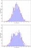 |
Fig. 2 Top histogram: simulated sample of size N = 1000 drawn from a superposition of two Gaussian distributions separated by r = 2.0 standard deviations. The solid curve is the best-fitting single Gaussian. In this case the null hypothesis, that the sample was drawn from a single Gaussian, cannot be rejected. Bottom histogram: simulation with separation r = 2.4 standard deviations. The solid curve is again the best-fitting single Gaussian. In this case the null hypothesis would be rejected and a much better fit could be obtained by fitting two Gaussians (not shown). |
The two simulated samples in Fig. 2 illustrate the situation for N = 1000. In the top diagram (generated with r = 2.0) it is not possible to conclude that there are two populations, while in the bottom one (for r = 2.4) they are rather clearly distinguished.
Given the data x = (x1, x2, ..., xN) we now compute a test statistic t(x) quantifying how much the data deviate from the distribution assumed under the null hypothesis, i.e., in this case a Gaussian with mean value μ and standard deviation σ (both of which must be estimated from the data). A large value of t indicates that the data do not follow this distribution. The null hypothesis is consequently rejected if t(x) exceeds some critical value C, chosen such that the probability of falsely rejecting H0 is some suitably small number, say α = 0.01 (the significance of the test).
It should be noted that H0 and HA are not complementary, i.e., if H0 is rejected it does not automatically follow that HA should be accepted. Indeed, there are obviously many possible distributions of X that cannot be described by either H0 or HA. Having rejected H0, the next logical step is to test whether HA provides a reasonable explanation of the data, or if that hypothesis, too, has to be rejected. However, since we are specifically interested in detecting substructures in the distribution of X, of which HA provides the simplest possible example, it is very relevant to examine how powerful the chosen test is in rejecting H0, when HA is true, as a function of N and r.
The test statistic t(x) measures the “distance” of the data from the best-fitting normal (Gaussian) distribution with free parameters μ and σ. Numerous tests for “normality” exist, but many of them are quite sensitive to outliers (indeed, some are constructed to detect outliers) and therefore unsuitable for our application. Instead we make use of the distance measure D from the well-known Kolmogorov–Smirnov (K–S) one-sample test (Press et al. 2007), which is relatively insensitive to outliers and readily adapted to non-Gaussian distributions, if needed. We define  (1)where FN is the empirical distribution function for the given data (i.e., FN(x; x) = n(x)/N, where n(x) is the number of data points ≤x) and F(x; μ,σ) is the normal cumulative distribution function for mean value μ and standard deviation σ. The expression in Eq. (1) requires some explanation. The quantity obtained as the maximum of the absolute difference between the two cumulative distributions is the distance measure D used in the standard one-sample K–S test. This D is however a function of the parameters of the theoretical distribution, in this case μ and σ, and we therefore adjust these parameters to give the minimum D. This is multiplied by
  to make the distribution of t under H0 nearly independent of N, and to avoid inconveniently small values of D for large samples.
The distribution of t(x) for given N and r must be determined through Monte-Carlo simulations, in which many independent realizations of x are generated and t computed for each of them by application of Eq. (1)3. We give results for some selected combinations of (N,r) in Fig. 3. Each curve in these diagrams shows the fraction of t-values exceeding C in a simulation with 2000 realizations of x. The fractions are plotted on a non-linear vertical scale (using a log [P/(1 − P)] transformation) in order to highlight both tails of the distribution. The wiggles in the upper and lower parts of the curves are caused by the number statistics due to the limited number of realizations.
For a given value of C, the significance of the test, i.e., the probability of falsely rejecting H0 (“Type I error”), can be directly read off the solid curves in Fig. 3 as α = P(t > C; r = 0). Conversely, we can determine the C-value to be used for a given significance level. Adopting a relatively conservative α = 0.01 we find that C ≃ 0.7 can be used for any sample size. For r > 0 the dashed curves give the power 1 − β of the test, where β is the probability of a “Type II error”, i.e., of failing to reject H0 when HA is true. For example, if we require 1 − β ≥ 0.99 at C = 0.7, the minimum r that is detected with this high degree of probability is about 4.2, 2.5, and 1.7 for the sample sizes shown in Fig. 3. For the two specific examples in Fig. 2 the computed statistic is t = 0.41 (top) and 1.04 (bottom), meaning that H0 would be rejected at the 1% significance level in the latter case, but not in the former.
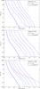 |
Fig. 3 Examples of probability plots for the test statistic t(x) obtained in Monte-Carlo simulations for sample sizes N = 102, 103, and 104 (top to bottom). In each diagram the solid curve shows, as a function of the critical value C, the probability that t exceeds C under the null hypothesis (r = 0). The dashed curves show the probabilities under the alternative hypothesis (r > 0) for the r-values indicated in the legend. In the bottom diagram the dotted curve gives, for comparison, the expected distribution of |
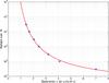 |
Fig. 4 Minimum sample size needed to distinguish two equal Gaussian populations, as a function of the separation of the population mean in units of the standard deviation of each population. The circles are the results from Monte-Carlo simulations as described in the text, using a K–S type test with significance level α = 0.01 and power 1 − β = 0.99. The curve is the fitted function in Eqs. (2) or (3). |
Results are summarized in Fig. 4, which shows the minimum sample size as a function of r for the assumptions described above. The circles are the results of the Monte-Carlo simulations for α = 0 and 1 − β = 0.99, obtained by interpolating in Fig. 3 and the corresponding diagrams for N = 30, 300, 3000, and 30 000. The curve is the fitted function 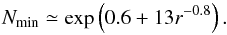 (2)This function, which has no theoretical foundation and therefore should not be used outside of the experimental range (30 ≤ N ≤ 30 000), can be inverted to give the minimum separation for a given sample size:
 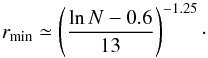 (3)For example, if the populations are separated by 5 times the measurement error (r = 5), the populations could be separated already for N ≃ 70. For r = 3 the minimum sample size is N = 400, and for r = 2 it is N = 3000. Clearly, if the separation is about the same as the measurement errors (r = 1), the situation is virtually hopeless even if the sample includes hundreds of thousands of stars.
It should be remembered that these results were obtained with a very specific set of assumptions, including: (1) measurement errors (and/or internal scatter) that are purely Gaussian; (2) that the two populations in the alternative hypothesis are equally large; (3) the use of the particular statistic in Eq. (1); and (4) the choice of significance (a probability of falsely rejecting H0 less than α = 0.01) and power (a probability of correctly rejecting H0 greater than 1 − β = 0.99). Changing any of these assumptions would result in a different relation4 from the one shown in Fig. 4. Nevertheless, this investigation already indicates how far we can go in replacing spectroscopic resolution and signal-to-noise ratios (i.e., small measurement errors) with large-number statistics. In particular when we consider that real data are never as clean, nor the expected abundance patterns as simple as assumed here, our estimates must be regarded as lower bounds to what can realistically be achieved.
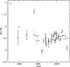 |
Fig. 5 Updated plot for HD 140283 from Gustafsson (2004). On the y axis are shown the [Fe/H] values determined from spectroscopy as reported in the literature. The x axis gives the year of the publication. The error bars indicate (full lines) the line-to-line scatter (when available) and (dotted lines) a few examples of attempts to address the full error including errors in the stellar parameters. The circles (°, at 1996) refer to a single analysis using three different temperature scales and the cross (×) refers to an analysis of a high-resolution spectrum using the SEGUE pipeline (Lee et al. 2011, see also Sect. 4 for database usage). |
4. Accuracy and precision in stellar abundances
We have no knowledge a priori of the properties of a star and no experiment to manipulate in the laboratory but can only observe the emitted radiation and from that infer the stellar properties. Therefore the accuracy5 of elemental abundances in stars is often hard to ascertain as it depends on a number of physical effects and properties that are not always well-known, well-determined, or well-studied (Baschek 1991). Important examples of relevant effects include deviations from local thermodynamic equilibrium (NLTE) and deviations from 1D geometry (Asplund 2005; Heiter & Eriksson 2006). Additionally, systematic and random errors in the stellar parameters will further decrease the accuracy as well as the precision within a study.
An interesting example of the slow convergence of the derived iron abundance in spite of increasing precision is given in Gustafsson (2004), where he compares literature results for the well studied metal-poor sub-giant HD 142083. Over time the error-bars resulting from line-to-line scatter decreases thanks to increased wavelength coverage (i.e., more Fe i lines are used in the analysis) and higher signal-to-noise ratios. However, the differences between studies remain large. An updated and augmented version of the plot in Gustafsson (2004) is given in Fig. 5. Data were sourced using SIMBAD and the SAGA database (Suda et al. 2008). For data listed in the SAGA database we excluded all non-unique data, e.g., where a value for [Fe/H] is quoted but that value is not determined in the study in question but taken from a previous study. The error bars shown are measures of the precision based on the quality of the spectra and reflect the line-to-line scatter. Generally, the precision has clearly improved with time, but, judging from the scatter between different determinations, it is doubtful if the overall accuracy has improved much. From around 1995 most studies quote a precision from measurement errors and errors in log gf values alone of 0.1 dex. From about the same time there appears also to be a convergence on two different [Fe/H] values. The difference is mainly related to a high and a low value of log g, whilst Teff appears uncorrelated with this split in [Fe/H] values. This illustrates the need for homogeneous samples treated in the same consistent way if substructures should be detected. Combining data from many different studies may in fact create unphysical structures in abundance space.
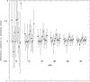 |
Fig. 6 Results from Lee et al. (2008). We plot the difference between the final abundance adopted in Lee et al. (2008) and the abundance derived using one of eleven methods (as described in Lee et al. 2008) as a function of the signal-to-noise ratio. The error bar shows the scatter for each method. |
An example of a homogeneous treatment of a large number of stars is the SEGUE survey6. An interesting illustration of the (inherent?) difficulties in reaching accurate results is given by the first paper on the SSPS pipeline used to analyse the SEGUE spectra (Lee et al. 2008). The pipeline implements eleven methods to derive iron abundances. Figure 6 summarizes the resulting differences between the adopted iron abundance and those derived using the eleven different methods as a function of signal-to-noise ratios in the stellar spectra. Most of the methods converge towards the adopted value around a signal-to-noise ratio of about 25, where the typical scatter for any of the methods is about 0.1 dex. However, there are methods that give iron abundances that deviate systematically by a similar amount also at higher signal-to-noise ratios, even though in this case the underlying assumptions are quite uniform. Thus this comparison suggests that the precision (as judged from the scatter of individual methods) is about 0.1 dex, and that systematic errors could be at least as large.
It is possible to access the precision in the derived elemental abundances with a full forward modelling of the analysis of a stellar spectrum. This can be done as a preparatory step for instrument designs. A recent example is given by Caffau et al. (2013) who ran model spectra through a simulator built to resemble the 4MOST multi-object spectrograph for VISTA (de Jong et al. 2012). The simulator includes a transmission model of the Earth’s atmosphere, a model for the seeing and sky background, and a simple model of the instrument. They found that they could reproduce the input abundance ratios with a precision of 0.1 dex for most elements and 0.2 dex for some elements.
We note with some interest that Eq. (3) fits results from recent works in the literature. For example, Nissen & Schuster (2010) used about 100 stars in their study, and rmin according to Eq. (3) is thus 4.4. Since their quoted precision is 0.04 dex for [Mg/Fe], the difference of about 0.2 dex seen in Fig. 1 is compatible with the prediction from Sect. 3 that the minimum discernible difference should be about rmin × σ = 0.17 dex. A similar comparison can be made for the results from SEGUE, e.g., as reported in Lee et al. (2011). With 17 000 stars rmin is 1.6. The quoted precision is no more than 0.1 dex in [α/Fe] which leads to rmin × σ = 0.16 dex. Figure 1 shows that the difference between the thin and the thick disk in the solar neighbourhood may be as large as 0.2 dex, hence the SEGUE spectra should be able to detect the difference between the two disks. Lee et al. (2011) do indeed find a clearly bimodal distribution in [α/Fe], although it may be less visible once the data are corrected for selection effects (Bovy et al. 2012). We note that even if the precision would be somewhat worse the situation is still good. These two studies nicely illustrate the trade-off between high precision and high numbers of stars. It also illustrates that our formula in Eq. (3) is a good representation of actual cases and can be used for decision making when planning a large survey or a small study.
A differential study is the best way to reach high precision (e.g., Gustafsson 2004; Baschek 1991; Magain 1984). One important aspect in the differential analysis is that measurement errors or erroneous theoretical calculation for log gf-values become irrelevant. The power of differential analysis has been amply exemplified over the past decades (e.g., Edvardsson et al. 1993; Bensby et al. 2004; Nissen & Schuster 2010). A very recent example are the studies of solar twins (Meléndez et al. 2012, who reached precisions of <0.01 dex). Such precision is possible because they study solar twins – all the stars have very similar stellar parameters. This means that erroneous treatment of the stellar photosphere and the radiative transport, as well as erroneous log gf-values, cancel out to first order. This “trick” can be repeated for any type of star and has, e.g., been successfully applied to metal-poor dwarf stars (Magain 1984; Nissen et al. 2002; Nissen & Schuster 2010).
Most large studies must by necessity mix stars with different stellar parameters. However, in future large spectroscopic surveys it will be feasible, both at the survey design stage and in the interpretation of the data, to select and focus on stars with similar stellar parameters. Those smaller, but more precise stellar samples will yield more information on potential substructures in elemental abundance space than would be the case if all stars were lumped together in order up the number statistics.
5. Concluding remarks
With the advent of Gaia, the exploration of the Milky Way as a galaxy will take a quantum leap forward. We will be working in a completely new regime – that of Galactic precision astronomy. Gaia is concentrating on providing the best possible distances and proper motions for a billion objects across the Milky Way and beyond. For stars brighter than 17th magnitude radial velocities will also be supplied. However, for fainter stars no radial velocities will be obtained and thus no complete velocity vector will be available. No detailed elemental abundances will be available for any star based on the limited on-board facilities.
The Gaia project has therefore created significant activity also as concerns ground-based spectroscopic follow-up. A recent outcome of that is the approval of the Gaia-ESO Survey proposal, which has been given 300 nights on VLT (Gilmore et al. 2012). In Europe several studies are under way for massive ground based follow-up of Gaia including both low- and high-resolution spectra. The designs include multiplexes of up to 3000 fibres over field-of-views of up to 5 deg2 (de Jong et al. 2012; Cirasuolo et al. 2012; Balcells et al. 2010). A number of other projects are currently under way and will also contribute relevant data to complement Gaia, even though they were not always designed with Gaia in mind. Examples include the on-going APOGEE, which will observe about 100 000 giant stars down to H = 12.5 at high resolution in the near-infrared in the Bulge and Milky Way disk (Wilson et al. 2010), and LAMOST, which will cover large fractions of the Northern sky and especially the anti-center direction (Cui et al. 2012). Of particular interest to Gaia and to the European efforts is the GALAH survey, which will use the high-resolution optical multi-object HERMES spectrograph at AAT to do a large survey down to V = 14 (Heijmans et al. 2012). The promise of elemental abundances for hundreds of thousands to millions of stars across all major components of the Galaxy, spread over much larger distances than ever before, is very exciting. Here we have investigated which types of substructures in abundance space that could be distinguished with these observations.
Clearly the arguments presented in Sect. 3 show that it is mandatory to strive for the best possible precision in the abundance measurements in order to detect stellar populations that differ in their elemental abundances from each other. Equation (2) gives an estimate of the number of stars needed to detect substructures in abundance space when the precision is known and can be used as a tool for trade-offs between number statistics and precision when planning large surveys.
The term “precision” refers to the ability of a method to give the same result from repeated measurements (observations). See Sect. 4 and footnote 5 for the distinction between precision and accuracy.
The distribution of t under H0 does not follow the theoretical distribution of  usually given for the K–S test, i.e.,
 ![\hbox{$P(t>C)=Q_{\rm KS}[(1+0.12/\!\sqrt{N}+0.11/N)C]$}](/articles/aa/full_html/2013/05/aa21057-13/aa21057-13-eq83.png) , where the function QKS is given in Press et al. (2007). This distribution, shown as a dotted curve in the bottom diagram of Fig. 3, is clearly very different from the empirical distribution for r = 0 given by the solid curve in the same diagram. The reason is that the K–S test assumes that the comparison is made with a fixed distribution F(x). In our case we adjust μ and σ to minimize , which results in a different distribution.
, where the function QKS is given in Press et al. (2007). This distribution, shown as a dotted curve in the bottom diagram of Fig. 3, is clearly very different from the empirical distribution for r = 0 given by the solid curve in the same diagram. The reason is that the K–S test assumes that the comparison is made with a fixed distribution F(x). In our case we adjust μ and σ to minimize , which results in a different distribution.
“Accuracy” refers to the capability of a method to return the correct result of a measurement, in contrast to precision which only implies agreement between the results of different measurements. It is possible to have high precision but poor accuracy, as is often the case in astronomy. For the purpose of the study of trends in elemental abundances in the Milky Way both are important, but for practical reasons most studies are concerned with precision rather than accuracy.
SEGUE is the Sloan Extension for Galactic Understanding and Exploration to map the structure and stellar makeup of the Milky Way Galaxy using the 2.5 m telescope at Apache point (Yanny et al. 2009).
Acknowledgments
This project was supported by grant Dnr 106:11 from the Swedish Space Board (LL) and by grant number 2011-5042 from The Swedish Research Council (SF). This research made use of the SIMBAD database, operated at CDS, Strasbourg, France and the SAGA database (Suda et al. 2008).
References
- Adibekyan, V. Z., Sousa, S. G., Santos, N. C., et al. 2012, A&A, 545, A32 [NASA ADS] [CrossRef] [EDP Sciences] [Google Scholar]
- Asplund, M. 2005, ARA&A, 43, 481 [NASA ADS] [CrossRef] [Google Scholar]
- Balcells, M., Benn, C. R., Carter, D., et al. 2010, in SPIE Conf. Ser., 7735, 77357 [Google Scholar]
- Baschek, B. 1991, in Evolution of Stars: the Photospheric Abundance Connection, eds. G. Michaud, & A. V. Tutukov, IAU Symp., 145, 39 [Google Scholar]
- Bensby, T., Feltzing, S., & Lundström, I. 2004, A&A, 415, 155 [NASA ADS] [CrossRef] [EDP Sciences] [Google Scholar]
- Bensby, T., Feltzing, S., Lundström, I., & Ilyin, I. 2005, A&A, 433, 185 [NASA ADS] [CrossRef] [EDP Sciences] [Google Scholar]
- Bovy, J., Rix, H.-W., & Hogg, D. W. 2012, ApJ, 751, 131 [NASA ADS] [CrossRef] [Google Scholar]
- Caffau, E., Koch, A., Sbordone, L., et al. 2013, Astron. Nachr., 334, 197 [NASA ADS] [Google Scholar]
- Cirasuolo, M., Afonso, J., Bender, R., et al. 2012, in SPIE Conf. Ser., 8446, 84460S [Google Scholar]
- Cui, X.-Q., Zhao, Y.-H., Chu, Y.-Q., et al. 2012, Res. Astron. Astrophys., 12, 1197 [NASA ADS] [CrossRef] [Google Scholar]
- de Jong, R. S., Bellido-Tirado, O., Chiappini, C., et al. 2012, in SPIE Conf. Ser., 8446, 84460T [Google Scholar]
- Edvardsson, B., Andersen, J., Gustafsson, B., et al. 1993, A&A, 275, 101 [NASA ADS] [Google Scholar]
- Freeman, K., & Bland-Hawthorn, J. 2002, ARA&A, 40, 487 [NASA ADS] [CrossRef] [Google Scholar]
- Fuhrmann, K. 1998, A&A, 338, 161 [NASA ADS] [Google Scholar]
- Fuhrmann, K. 2000, unpublished [Google Scholar]
- Fuhrmann, K. 2002, New Astron., 7, 161 [NASA ADS] [CrossRef] [Google Scholar]
- Fuhrmann, K. 2004, Astron. Nachr., 325, 3 [NASA ADS] [CrossRef] [MathSciNet] [Google Scholar]
- Fuhrmann, K. 2008, MNRAS, 384, 173 [NASA ADS] [CrossRef] [Google Scholar]
- Fuhrmann, K. 2011, MNRAS, 414, 2893 [NASA ADS] [CrossRef] [Google Scholar]
- Gilmore, G., Randich, S., Asplund, M., et al. 2012, The Messenger, 147, 25 [NASA ADS] [Google Scholar]
- Gustafsson, B. 2004, in Origin and Evolution of the Elements, eds. A. McWilliam, & M. Rauch, Carnegie Observatories Astrophysics Series, 4, 102 [Google Scholar]
- Heijmans, J., Asplund, M., Barden, S., et al. 2012, in SPIE Conf. Ser., 8446, 84460 [Google Scholar]
- Heiter, U., & Eriksson, K. 2006, A&A, 452, 1039 [NASA ADS] [CrossRef] [EDP Sciences] [Google Scholar]
- Lee, Y. S., Beers, T. C., Sivarani, T., et al. 2008, AJ, 136, 2022 [NASA ADS] [CrossRef] [Google Scholar]
- Lee, Y. S., Beers, T. C., An, D., et al. 2011, ApJ, 738, 187 [NASA ADS] [CrossRef] [Google Scholar]
- Magain, P. 1984, A&A, 132, 208 [NASA ADS] [Google Scholar]
- Majewski, S. R., Wilson, J. C., Hearty, F., Schiavon, R. R., & Skrutskie, M. F. 2010, in IAU Symp. 265, eds. K. Cunha, M. Spite, & B. Barbuy, 480 [Google Scholar]
- Meléndez, J., Bergemann, M., Cohen, J. G., et al. 2012, A&A, 543, A29 [NASA ADS] [CrossRef] [EDP Sciences] [Google Scholar]
- Neves, V., Santos, N. C., Sousa, S. G., Correia, A. C. M., & Israelian, G. 2009, A&A, 497, 563 [NASA ADS] [CrossRef] [EDP Sciences] [Google Scholar]
- Nissen, P. E., & Schuster, W. J. 2010, A&A, 511, L10 [NASA ADS] [CrossRef] [EDP Sciences] [Google Scholar]
- Nissen, P. E., Primas, F., Asplund, M., & Lambert, D. L. 2002, A&A, 390, 235 [NASA ADS] [CrossRef] [EDP Sciences] [Google Scholar]
- Press, W., Teukolsky, S., Vetterling, W., & Flannery, B. 2007, Numerical Recipes: The Art of Scientific Computing, 3rd edn. (Cambridge University Press) [Google Scholar]
- Reddy, B. E., Tomkin, J., Lambert, D. L., & Allen de Prieto, C. 2003, MNRAS, 340, 304 [NASA ADS] [CrossRef] [Google Scholar]
- Reddy, B. E., Lambert, D. L., & Allen de Prieto, C. 2006, MNRAS, 367, 1329 [NASA ADS] [CrossRef] [Google Scholar]
- Suda, T., Katsuta, Y., Yamada, S., et al. 2008, PASJ, 60, 1159 [NASA ADS] [Google Scholar]
- Tolstoy, E., Hill, V., & Tosi, M. 2009, ARA&A, 47, 371 [NASA ADS] [CrossRef] [Google Scholar]
- Wilson, J. C., Hearty, F., Skrutskie, M. F., et al. 2010, in SPIE Conf. Ser., 7735, 77351 [Google Scholar]
- Yanny, B., Rockosi, C., Newberg, H. J., et al. 2009, AJ, 137, 4377 [NASA ADS] [CrossRef] [Google Scholar]
- Zwitter, T., Siebert, A., Munari, U., et al. 2008, AJ, 136, 421 [NASA ADS] [CrossRef] [Google Scholar]
All Figures
|
Fig. 1 Illustration of the problem, showing Fe and Mg abundances for stars in the solar neighbourhood. a) Based on data by Fuhrmann (see text for references). At each value of [Fe/H] the stars fall into two groups with distinctly different [Mg/Fe]. b) Based on data for stars with halo velocities from Nissen & Schuster (2010). The two lines, drawn by hand, illustrate the separation in high- and low-α stars identified by Nissen & Schuster (2010). c) Illustration of the generic problem treated here. |
| In the text | |
|
Fig. 2 Top histogram: simulated sample of size N = 1000 drawn from a superposition of two Gaussian distributions separated by r = 2.0 standard deviations. The solid curve is the best-fitting single Gaussian. In this case the null hypothesis, that the sample was drawn from a single Gaussian, cannot be rejected. Bottom histogram: simulation with separation r = 2.4 standard deviations. The solid curve is again the best-fitting single Gaussian. In this case the null hypothesis would be rejected and a much better fit could be obtained by fitting two Gaussians (not shown). |
| In the text | |
|
Fig. 3 Examples of probability plots for the test statistic t(x) obtained in Monte-Carlo simulations for sample sizes N = 102, 103, and 104 (top to bottom). In each diagram the solid curve shows, as a function of the critical value C, the probability that t exceeds C under the null hypothesis (r = 0). The dashed curves show the probabilities under the alternative hypothesis (r > 0) for the r-values indicated in the legend. In the bottom diagram the dotted curve gives, for comparison, the expected distribution of |
| In the text | |
|
Fig. 4 Minimum sample size needed to distinguish two equal Gaussian populations, as a function of the separation of the population mean in units of the standard deviation of each population. The circles are the results from Monte-Carlo simulations as described in the text, using a K–S type test with significance level α = 0.01 and power 1 − β = 0.99. The curve is the fitted function in Eqs. (2) or (3). |
| In the text | |
|
Fig. 5 Updated plot for HD 140283 from Gustafsson (2004). On the y axis are shown the [Fe/H] values determined from spectroscopy as reported in the literature. The x axis gives the year of the publication. The error bars indicate (full lines) the line-to-line scatter (when available) and (dotted lines) a few examples of attempts to address the full error including errors in the stellar parameters. The circles (°, at 1996) refer to a single analysis using three different temperature scales and the cross (×) refers to an analysis of a high-resolution spectrum using the SEGUE pipeline (Lee et al. 2011, see also Sect. 4 for database usage). |
| In the text | |
|
Fig. 6 Results from Lee et al. (2008). We plot the difference between the final abundance adopted in Lee et al. (2008) and the abundance derived using one of eleven methods (as described in Lee et al. 2008) as a function of the signal-to-noise ratio. The error bar shows the scatter for each method. |
| In the text | |
Current usage metrics show cumulative count of Article Views (full-text article views including HTML views, PDF and ePub downloads, according to the available data) and Abstracts Views on Vision4Press platform.
Data correspond to usage on the plateform after 2015. The current usage metrics is available 48-96 hours after online publication and is updated daily on week days.
Initial download of the metrics may take a while.