| Issue |
A&A
Volume 553, May 2013
|
|
|---|---|---|
| Article Number | A29 | |
| Number of page(s) | 9 | |
| Section | Extragalactic astronomy | |
| DOI | https://doi.org/10.1051/0004-6361/201220324 | |
| Published online | 25 April 2013 | |
Luminosity-dependent unification of active galactic nuclei and the X-ray Baldwin effect
1
ISDC Data Centre for
Astrophysics, Université de Genève, ch. d’Ecogia 16, 1290
Versoix,
Switzerland
2
Observatoire de Genève, Université de Genève,
51 Ch. des
Maillettes, 1290
Versoix,
Switzerland
3
Department of Astronomy, Kyoto University,
Oiwake-cho, Sakyo-ku, 606-8502
Kyoto,
Japan
e-mail: This email address is being protected from spambots. You need JavaScript enabled to view it.
4
Department of Physics, Ehime University,
790-8577
Matsuyama,
Japan
5
UJF-Grenoble 1/CNRS-INSU, Institut de Planétologie et
d’Astrophysique de Grenoble (IPAG) UMR 5274, 38041
Grenoble,
France
6
Max-Planck-Institut für extraterrestrische Physik,
Giessenbachstrasse
1, 85748
Garching bei München,
Germany
Received:
3
September
2012
Accepted:
31
January
2013
Abstract
The existence of an anti-correlation between the equivalent width (EW) of the narrow core of the iron Kα line and the luminosity of the continuum (i.e., the X-ray Baldwin effect) in type I active galactic nuclei has been confirmed in recent years by several studies carried out with XMM-Newton, Chandra and Suzaku. However, no general consensus on the origin of this trend has been reached so far. Several works have proposed the decrease of the covering factor of the molecular torus with the luminosity (in the framework of the luminosity-dependent unification models) as a possible explanation for the X-ray Baldwin effect. Using the fraction of obscured sources measured by recent X-ray and infrared (IR) surveys as a proxy of the half-opening angle of the torus and recent Monte Carlo simulations of the X-ray radiation reprocessed by a structure with a spherical-toroidal geometry, we test the hypothesis that the X-ray Baldwin effect is related to the decrease of the half-opening angle of the torus with the luminosity. Simulating the spectra of an unabsorbed population with a luminosity-dependent covering factor of the torus as predicted by recent X-ray surveys, we find that this mechanism is able to explain the observed X-ray Baldwin effect. Fitting the simulated data with a log-linear L2−10 keV − EW relation, we found that in the Seyfert regime (L2−10 keV ≤ 1044.2 erg s-1) luminosity-dependent unification produces a slope consistent with the observations for average values of the equatorial column densities of the torus of log NHT ≳ 23.2, and can reproduce both the slope and the intercept for log NHT ≃ 23.2. Lower values of NHT are obtained assuming the decrease of the covering factor of the torus with the luminosity extrapolated from IR observations (22.9 ≲ log NHT ≲ 23). In the quasar regime (L 2−10 keV > 1044.2 erg s-1), a decrease of the covering factor of the torus with the luminosity slower than that observed in the Seyfert regime (as found by recent hard X-ray surveys) is able to reproduce the observations for 23.2 ≲ log NHT ≲ 24.2.
Key words: galaxies: Seyfert / quasars: general / galaxies: active / X-rays: galaxies
© ESO, 2013
1. Introduction
There are two main observational signatures of reprocessed radiation in the X-ray spectra of active galactic nuclei (AGN): a Compton hump peaking around 30 keV and a fluorescent iron Kα line. While the Compton hump is produced only if the reprocessing material is Compton thick (CT, N H ≳ 1024 cm-2), the iron Kα line is also created in Compton-thin material (e.g., Matt et al. 2003). The iron Kα line is often observed as the superposition of two different components: a broad component and a narrow one. The broad component has a full width at half-maximum (FWHM) of ≳30 000 km s and is thought to be created close to the black hole in the accretion disk (e.g., Fabian et al. 2000), or to be related to the presence of features created by partially covering warm absorbers in the line of sight (e.g., Turner & Miller 2009; Miyakawa et al. 2012). While the broad component is observed in only ~35–45% of bright nearby AGN (e.g., de La Calle Pérez et al. 2010), the narrow (FWHM ~ 2000 km s, Shu et al. 2010) core of the iron line has been found to be almost ubiquitous (e.g., Nandra et al. 2007; Singh et al. 2011). This component peaks at 6.4 keV (e.g.,Yaqoob & Padmanabhan 2004), which points to the line being produced in cold neutral material. This material has often been identified as circumnuclear matter located at several thousand gravitational radii from the supermassive black hole, and it is likely related to the putative molecular torus (e.g., Nandra 2006), although a contribution of the outer part of the disk (e.g., Petrucci et al. 2002) or of the broad-line region (BLR, e.g., Bianchi et al. 2008) cannot be excluded. In a recent study, Shu et al. (2011) found that the weighted mean of the ratio between the FWHM of the narrow Fe Kα line and that of optical lines produced in the BLR is ≃ 0.6. This implies that the size of the iron Kα-emitting region is on average about three times that of the BLR, indicating that most of the narrow iron Kα emission is produced in the putative molecular torus.
Summary of the most recent studies (along with the original work of Iwasawa & Taniguchi 1993) of the X-ray Baldwin effect.
One of the most interesting characteristics of the narrow component of the iron Kα line is the inverse correlation between its equivalent width (EW) and the X-ray luminosity (e.g., Iwasawa & Taniguchi 1993). The existence of an anti-correlation between the EW of a line and the luminosity of the AGN continuum was found for the first time in the UV by Baldwin (1977) for the C IV λ1549 line and dubbed the Baldwin effect. A similar trend was later found for several other emission lines, such as Lyα, [C III] λ1908, Si IV λ1396, Mg II λ2798 (Dietrich et al. 2002), UV iron emission lines (Green et al. 2001), mid-infrared (mid-IR) lines such as [AR III] λ8.99 μm, [S IV] λ10.51 μm and [Ne II] λ12.81 μm (Hönig et al. 2008), and forbidden lines such as [O II] λ3727 and [Ne V] λ3426 (Croom et al. 2002). The slope of the Baldwin effect for most of these lines has been shown to be steeper for the lines originating from higher ionization species (e.g., Dietrich et al. 2002). The origin of the Baldwin effect is still unknown, although several possible explanations have been put forward, and might be different for lines originating in different regions of the AGN. For the lines produced in the BLR, the origin might be related to the lower ionization and photoelectric heating in the BLR gas of more luminous objects (e.g., Netzer et al. 1992).
Using Ginga observations of 37 AGN, Iwasawa & Taniguchi (1993) found in the X-rays the first evidence of an
anti-correlation between the EW of the iron Kα line and the 2–10 keV
luminosity ( ).
This trend is usually called the X-ray Baldwin effect or
the Iwasawa-Taniguchi effect. Using ASCA observations, Nandra et al. (1997) confirmed the existence of such an
anti-correlation and argued that most of the effect could be explained by variations of the
broad component of the iron Kα line with the luminosity. The advent of
XMM-Newton, Chandra, and Suzaku made
clear however that most of the observed X-ray Baldwin effect is due to the narrow core of
the iron Kα line (e.g., Page et al.
2004; Shu et al. 2010; Fukazawa et al. 2011). The significance of the effect was questioned by
Jiménez-Bailón et al. (2005), who discussed the
possible importance of contamination from radio-loud (RL) AGN, which have on average larger
X-ray luminosities and smaller signatures of reprocessed radiation (e.g., Reeves & Turner 2000). However, Grandi et al. (2006), studying BeppoSAX
observations of RL AGN, also found evidence of an X-ray Baldwin effect. This,
together with the study of a large sample of radio-quiet (RQ) AGN carried out by Bianchi et al. (2007) using XMM-Newton
data, showed that the X-ray Baldwin effect is not a mere artifact. Jiang et al. (2006) suggested that the X-ray Baldwin effect might be due
to the delay between the variability of the AGN primary energy source and that of the
reprocessing material located farther away. Using Chandra/HEG observations,
Shu et al. (2010, 2012) confirmed the importance of variability, showing that averaging the values
of EW obtained over multiple observations of individual sources would significantly
attenuate the anti-correlation from
).
This trend is usually called the X-ray Baldwin effect or
the Iwasawa-Taniguchi effect. Using ASCA observations, Nandra et al. (1997) confirmed the existence of such an
anti-correlation and argued that most of the effect could be explained by variations of the
broad component of the iron Kα line with the luminosity. The advent of
XMM-Newton, Chandra, and Suzaku made
clear however that most of the observed X-ray Baldwin effect is due to the narrow core of
the iron Kα line (e.g., Page et al.
2004; Shu et al. 2010; Fukazawa et al. 2011). The significance of the effect was questioned by
Jiménez-Bailón et al. (2005), who discussed the
possible importance of contamination from radio-loud (RL) AGN, which have on average larger
X-ray luminosities and smaller signatures of reprocessed radiation (e.g., Reeves & Turner 2000). However, Grandi et al. (2006), studying BeppoSAX
observations of RL AGN, also found evidence of an X-ray Baldwin effect. This,
together with the study of a large sample of radio-quiet (RQ) AGN carried out by Bianchi et al. (2007) using XMM-Newton
data, showed that the X-ray Baldwin effect is not a mere artifact. Jiang et al. (2006) suggested that the X-ray Baldwin effect might be due
to the delay between the variability of the AGN primary energy source and that of the
reprocessing material located farther away. Using Chandra/HEG observations,
Shu et al. (2010, 2012) confirmed the importance of variability, showing that averaging the values
of EW obtained over multiple observations of individual sources would significantly
attenuate the anti-correlation from  to
to
 .
Chandra/HEG observations (Shu et al.
2010) have also shown that the normalization of the X-ray Baldwin effect is lower
(i.e., the average EW of the narrow Fe Kα component is smaller) than that
obtained by previous works performed using XMM-Newton. In Table 1 we report the values of the slope and the intercept
obtained from the most recent XMM-Newton/EPIC and
Chandra/HEG works, along with the original Ginga work of
Iwasawa & Taniguchi (1993).
.
Chandra/HEG observations (Shu et al.
2010) have also shown that the normalization of the X-ray Baldwin effect is lower
(i.e., the average EW of the narrow Fe Kα component is smaller) than that
obtained by previous works performed using XMM-Newton. In Table 1 we report the values of the slope and the intercept
obtained from the most recent XMM-Newton/EPIC and
Chandra/HEG works, along with the original Ginga work of
Iwasawa & Taniguchi (1993).
An intriguing possibility is that the X-ray Baldwin effect is related to the decrease of the covering factor of the torus with luminosity (e.g., Page et al. 2004; Zhou & Wang 2005) in the frame of the luminosity-dependent unification schemes. The EW of the iron Kα line is in fact expected to be proportional to the covering factor of the torus (e.g., Krolik et al. 1994, Ikeda et al. 2009), so that a covering factor of the torus decreasing with the luminosity might in principle be able to explain the X-ray Baldwin effect. Luminosity-dependent unification models have been proposed to explain the decrease of the fraction of obscured objects (fobs) with the increase of the AGN output power. The first suggestion of the existence of a relation between fobs and the luminosity was put forward about 30 years ago (Lawrence & Elvis 1982). Since then the idea that the covering factor of the obscuring material decreases with luminosity has been gaining observational evidence from radio (e.g., Grimes et al. 2004), infrared (e.g., Treister et al. 2008; Mor et al. 2009; Gandhi et al. 2009), optical (e.g., Simpson 2005), and X-ray (e.g., Ueda et al. 2003; Beckmann et al. 2009; Ueda et al. 2011) studies of AGN. Although luminosity-dependent unification models have long been suspected to play a major role in the X-ray Baldwin effect, no quantitative estimation of this effect has been performed so far.
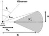 |
Fig. 1 Schematic representation of the torus geometry considered. The angle
θ i is the inclination of the line of sight with
respect to the torus axis, while θOA and
|
In this work we quantify for the first time the influence of the decrease of the covering factor of the torus with the luminosity on the EW of the iron Kα line. Using the Monte Carlo spectral simulations of a torus with a variable half-opening angle (θOA) (recently presented by Ikeda et al. 2009 and Brightman & Nandra 2011) together with the most recent and comprehensive observations in different energy bands of the decrease of fobs with the luminosity, we show that this mechanism is able to explain the X-ray Baldwin effect. The paper is organized as follows. In Sect. 2 we present in detail our spectral simulations, and in Sect. 3 we compare the slopes and intercepts obtained by our simulations with those measured by high-sensitivity Chandra/HEG observations, as they provide the best energy resolution available to date. In Sect. 4 we discuss our results, and in Sect. 5 we present our conclusions.
2. Simulations
2.1. The relation between θOA and L
As a proxy of the relationship between the half-opening angle of the molecular torus
θOA (see Fig. 1) and
the intrinsic X-ray luminosity of AGN, we used the variation of the fraction of obscured
sources fobs with luminosity measured by the recent medium
(2–10 keV) and hard (15–55 keV) X-ray surveys of Hasinger
(2008) and Burlon et al. (2011). From a
combination of surveys performed by HEAO-1, ASCA, BeppoSAX,
XMM-Newton, and Chandra in the luminosity range
42 ≤ log LX ≤ 46, Hasinger
(2008) found in the 2–10 keV band  (1)where
LX is the luminosity in the 2–10 keV energy range. In the
15–55 keV band, using Swift/BAT to study AGN in the luminosity range
42 ≤ log LX ≤ 45 and fitting the data with
(1)where
LX is the luminosity in the 2–10 keV energy range. In the
15–55 keV band, using Swift/BAT to study AGN in the luminosity range
42 ≤ log LX ≤ 45 and fitting the data with  (2)where
LHX is the luminosity in the 15–55 keV band, Burlon et al. (2011) obtained
Rlow = 0.8, Rhigh = 0.2, and
LC = 1043.7 erg s. We also used the results of
the IR work of Maiolino et al. (2007), who found an
anti-correlation between the ratio
λLλ(6.7 μm)/λLλ(5100 Å)
and the [O III]λ5007 Å line luminosity. This trend was interpreted as an
effect of the decrease of the covering factor of the circumnuclear dust as a function of
luminosity, with fobs varying as
(2)where
LHX is the luminosity in the 15–55 keV band, Burlon et al. (2011) obtained
Rlow = 0.8, Rhigh = 0.2, and
LC = 1043.7 erg s. We also used the results of
the IR work of Maiolino et al. (2007), who found an
anti-correlation between the ratio
λLλ(6.7 μm)/λLλ(5100 Å)
and the [O III]λ5007 Å line luminosity. This trend was interpreted as an
effect of the decrease of the covering factor of the circumnuclear dust as a function of
luminosity, with fobs varying as 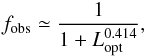 (3)where
Lopt = (λLλ(5100 Å))/1045.63.
Following Maiolino et al. (2007), it is possible to
rewrite Lopt as a function of the X-ray luminosity:
(3)where
Lopt = (λLλ(5100 Å))/1045.63.
Following Maiolino et al. (2007), it is possible to
rewrite Lopt as a function of the X-ray luminosity:
 .
.
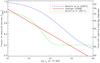 |
Fig. 2 Variation of the fraction of obscured sources (fobs) and of the half-opening angle of the torus (θOA) with the 2–10 keV luminosity for three of the most recent medium X-ray (2–10 keV, Hasinger 2008), hard X-ray (15–55 keV, Burlon et al. 2011), and IR (Maiolino et al. 2007) studies (Eqs. (1)–(3)). |
The fraction of obscured sources at a given luminosity can be easily related to the
half-opening angle of the torus using 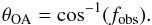 (4)For
Eq. (2) we converted the hard X-ray
luminosity to the luminosity in the 2–10 keV band, assuming a photon index Γ = 1.9 (e.g.,
Beckmann et al. 2009). The three
θOA − LX relationships used in
this work are shown in Fig. 2.
(4)For
Eq. (2) we converted the hard X-ray
luminosity to the luminosity in the 2–10 keV band, assuming a photon index Γ = 1.9 (e.g.,
Beckmann et al. 2009). The three
θOA − LX relationships used in
this work are shown in Fig. 2.
2.2. Spectral simulations and fitting
Ikeda et al. (2009) recently presented Monte Carlo
simulations of the reprocessed X-ray emission of an AGN surrounded by a three-dimensional
spherical-toroidal structure. The simulations were performed using the ray-tracing method,
taking into account Compton down-scattering and absorption. They are stored in tables, so
that they can be used to perform spectral fitting. The free parameters of this model are
the half-opening angle of the torus θOA, the line-of-sight
inclination angle θ i, the torus equatorial column density
 ,
and the photon index Γ of the primary continuum. We note that
should not be confused with the observed hydrogen column density
N H. In all objects,
,
and the photon index Γ of the primary continuum. We note that
should not be confused with the observed hydrogen column density
N H. In all objects,
 ,
with
,
with  only if θ i = 90°. In Fig. 1 a schematic representation of the geometry considered
is shown. The dependence of N H on the inclination angle is
given by Eq. (3) of Ikeda et al. (2009). In the
model of Ikeda et al. (2009), the
ratio Rin/R is fixed
to 0.01 and the inclination angle of the observer θi can vary
between 1 and 89°,
between 1022 and 1025 cm-2, while
θOA spans the range between 10°
and 70°. Because of the assumed dependence of the half-opening angle on the
luminosity, the interval of values of θOA allowed by the model
limits the range of luminosities we can probe. In the following we will consider
luminosities above log LX = 42, because below this value few
AGN are detected and several works point towards a possible disappearance of the molecular
torus (e.g., Elitzur & Shlosman 2006). The
upper-limit luminosity we can reach depends on the
θOA − LX relationship used and,
considering
only if θ i = 90°. In Fig. 1 a schematic representation of the geometry considered
is shown. The dependence of N H on the inclination angle is
given by Eq. (3) of Ikeda et al. (2009). In the
model of Ikeda et al. (2009), the
ratio Rin/R is fixed
to 0.01 and the inclination angle of the observer θi can vary
between 1 and 89°,
between 1022 and 1025 cm-2, while
θOA spans the range between 10°
and 70°. Because of the assumed dependence of the half-opening angle on the
luminosity, the interval of values of θOA allowed by the model
limits the range of luminosities we can probe. In the following we will consider
luminosities above log LX = 42, because below this value few
AGN are detected and several works point towards a possible disappearance of the molecular
torus (e.g., Elitzur & Shlosman 2006). The
upper-limit luminosity we can reach depends on the
θOA − LX relationship used and,
considering  , is
log L max = 44.2 for Hasinger (2008), log L max = 43.8 for Burlon et al. (2011), and
log L max = 45.0 for Maiolino et al. (2007). Due to its limitations in the values of
θOA permitted, the model of Ikeda et al. (2009) restricts most of the simulations to the Seyfert regime
(
, is
log L max = 44.2 for Hasinger (2008), log L max = 43.8 for Burlon et al. (2011), and
log L max = 45.0 for Maiolino et al. (2007). Due to its limitations in the values of
θOA permitted, the model of Ikeda et al. (2009) restricts most of the simulations to the Seyfert regime
( ).
).
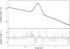 |
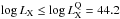
Fig. 3 Top panel: extract in the 5.5–7.5 keV region of a spectrum
simulated using the model of Ikeda et al.
(2009). The model has a torus with a half-opening angle of
θOA = 46.2° (equivalent to
log LX = 42.7, according to the relationship of Hasinger 2008), an equatorial column density of
|

To extend our study to the quasar regime ( ), we
simulated the X-ray Baldwin effect using the spectral model of Brightman & Nandra (2011). This model considers the same
geometry as Ikeda et al. (2009) but has
Rin = 0, a θ i-independent
N H, and it allows different values of
θOA (26° to 84°). The higher maximum
half-opening angle permitted by this model allows to reach higher maximum luminosities in
the simulations for the relationships of Hasinger
(2008;
log L max = 45.3) and Maiolino et al. (2007;
log L max = 46.2), while that of Burlon et al. (2011) is flat
(f obs ≃ 0.2) in the quasar regime. However, the lower
boundary of θOA in the model of Brightman & Nandra (2011) limits the lower luminosity we can reach in
the simulations, in particular log L min ≃ 43 for the
relation of Maiolino et al. (2007). Thus, we used
the model of Ikeda et al. (2009) to study the X-ray
Baldwin effect in the Seyfert regime (42 ≤ log LX ≤ 44.2) and
the model of Brightman & Nandra (2011) to
probe the quasar regime
(log LX > 44.2).
), we
simulated the X-ray Baldwin effect using the spectral model of Brightman & Nandra (2011). This model considers the same
geometry as Ikeda et al. (2009) but has
Rin = 0, a θ i-independent
N H, and it allows different values of
θOA (26° to 84°). The higher maximum
half-opening angle permitted by this model allows to reach higher maximum luminosities in
the simulations for the relationships of Hasinger
(2008;
log L max = 45.3) and Maiolino et al. (2007;
log L max = 46.2), while that of Burlon et al. (2011) is flat
(f obs ≃ 0.2) in the quasar regime. However, the lower
boundary of θOA in the model of Brightman & Nandra (2011) limits the lower luminosity we can reach in
the simulations, in particular log L min ≃ 43 for the
relation of Maiolino et al. (2007). Thus, we used
the model of Ikeda et al. (2009) to study the X-ray
Baldwin effect in the Seyfert regime (42 ≤ log LX ≤ 44.2) and
the model of Brightman & Nandra (2011) to
probe the quasar regime
(log LX > 44.2).
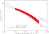 |
Fig. 4 Equivalent width of the iron Kα line versus the X-ray luminosity
obtained simulating a torus with an equatorial column density of
|
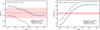 |
Fig. 5 Left panel: value of the slope (B) of the X-ray
Baldwin effect obtained simulating the variation of the reprocessed X-ray radiation
with the luminosity for tori with different values of the equatorial column density
|

To estimate the influence of the decreasing covering factor of the torus on the EW of the
iron line, we used the physical torus models to simulate a large number of spectra using
the θOA − LX relationships
reported in Eqs. (1)–(3). Using the three different
θOA − LX relationships, we
extrapolated the value of θOA for each luminosity bin
(Δlog LX = 0.01). We fixed the equatorial column density of
the torus
to 26 different values, spanning 1022.5 cm-2 and
1025 cm-2, with a step of  . To simulate an unabsorbed
population, similarly to what is usually used to determine the X-ray Baldwin effect, we
considered inclination angles θ i between 1° and
θOA for each value of L X and
,
with a binning of Δθ i = 3°. In XSPEC 12.7.1
(Arnaud 1996), we simulated spectra for each of
the three θOA − LX relationships
and for each bin of column density. For the continuum we used a power law with Γ = 1.9
(e.g., Beckmann et al. 2009). Our choice of the
photon index does not significantly affect the simulations; by adding a scatter of
ΔΓ = 0.3, we found EW − LX trends consistent
with those obtained without scatter. The metallicity was set to the solar value in all our
simulations, and the value of the normalization of the reflected component was fixed to
that of the continuum.
. To simulate an unabsorbed
population, similarly to what is usually used to determine the X-ray Baldwin effect, we
considered inclination angles θ i between 1° and
θOA for each value of L X and
,
with a binning of Δθ i = 3°. In XSPEC 12.7.1
(Arnaud 1996), we simulated spectra for each of
the three θOA − LX relationships
and for each bin of column density. For the continuum we used a power law with Γ = 1.9
(e.g., Beckmann et al. 2009). Our choice of the
photon index does not significantly affect the simulations; by adding a scatter of
ΔΓ = 0.3, we found EW − LX trends consistent
with those obtained without scatter. The metallicity was set to the solar value in all our
simulations, and the value of the normalization of the reflected component was fixed to
that of the continuum.
We fitted the simulated spectra in the 0.3–10 keV band using the same model applied for
the simulations, substituting the iron Kα line component with a Gaussian
line. We obtained a good fit for all the simulations, with a reduced chi-squared of
 . We
show in Fig. 3 an example of a typical fit. The model
used for the continuum fitting does not significantly affect the results, and the EW of
the iron Kα line differs only ~4% on average when using an alternative
model like pexrav (Magdziarz & Zdziarski
1995). We evaluated the EW of the iron Kα line and studied its
relationship with the luminosity. As an example, we show in Fig. 4 the simulated X-ray Baldwin effect obtained using the model of Ikeda et al. (2009) and the
θOA − LX relationship of Hasinger (2008) for
. We
show in Fig. 3 an example of a typical fit. The model
used for the continuum fitting does not significantly affect the results, and the EW of
the iron Kα line differs only ~4% on average when using an alternative
model like pexrav (Magdziarz & Zdziarski
1995). We evaluated the EW of the iron Kα line and studied its
relationship with the luminosity. As an example, we show in Fig. 4 the simulated X-ray Baldwin effect obtained using the model of Ikeda et al. (2009) and the
θOA − LX relationship of Hasinger (2008) for
 , together with the fit to
the X-ray Baldwin effect obtained by the recent works of Bianchi et al. (2007) and Shu et al.
(2012). The spread in EW for a given luminosity is due to the range of values of
θ i that we considered: larger values of EW usually
correspond to lower values of θ i.
, together with the fit to
the X-ray Baldwin effect obtained by the recent works of Bianchi et al. (2007) and Shu et al.
(2012). The spread in EW for a given luminosity is due to the range of values of
θ i that we considered: larger values of EW usually
correspond to lower values of θ i.
Most of the studies of the X-ray Baldwin effect performed in recent years have used a
relationship of the type  (5)to
fit the EW − LX trend, where
LX,44 is the luminosity in units of
1044 erg s. In order to compare the simulated
EW − LX trend with that observed in
unabsorbed populations of AGN, we fitted the simulated data, for each value
of ,
with Eq. (5) using the weighted
least-square method, with weights of
w = sinθ i. This makes it possible to
account for the non-uniform probability of randomly observing an AGN within a certain
solid angle from the polar axis.
(5)to
fit the EW − LX trend, where
LX,44 is the luminosity in units of
1044 erg s. In order to compare the simulated
EW − LX trend with that observed in
unabsorbed populations of AGN, we fitted the simulated data, for each value
of ,
with Eq. (5) using the weighted
least-square method, with weights of
w = sinθ i. This makes it possible to
account for the non-uniform probability of randomly observing an AGN within a certain
solid angle from the polar axis.
3. The X-ray Baldwin effect
Most of the studies on the X-ray Baldwin effect have found, using Eq. (5), a slope of B ~ −0.2 (e.g., Iwasawa & Taniguchi 1993; Page et al. 2004; Bianchi et al. 2007). However, in all these works the values of EW and LX are obtained from individual observations of sources. As pointed out by Jiang et al. (2006) and confirmed by Shu et al. (2010, 2012), flux variability might play an important role in the observed X-ray Baldwin effect. Shu et al. (2012) recently found a clear anti-correlation between the EW of the iron Kα line and the luminosity for individual sources that had several Chandra/HEG observations. Using a sample of 32 RQ AGN, they also found that the fit per source (i.e., averaging different observations of the same object) results in a significantly flatter slope (B = −0.11 ± 0.03) than that done per observation (i.e., using all the available observations for every source of the sample; B = −0.18 ± 0.03).
To compare the slope obtained by the simulations in the two different luminosity bands with real data, we fitted the data per source (33 AGN) of Shu et al. (2010; obtained fixing σ = 1 eV) with Eq. (5) in the Seyfert and quasar regime. Consistent with what was done by Shu et al. (2010) we did not use the three AGN for which only upper limits of EW were obtained. Using the 28 AGN in the Seyfert regime, we found that the best fit to the X-ray Baldwin effect is given by A = 1.64 ± 0.05 and B = −0.12 ± 0.04. Chandra/HEG observations are available for only five objects in the quasar regime, and at these luminosities we obtained A = 1.5 ± 0.3 and B = −0.16 ± 0.22.
 |
Fig. 6 Left panel: value of the slope (B) of the X-ray
Baldwin effect obtained simulating the variation of the reprocessed X-ray radiation
with the luminosity for tori with different values of the equatorial column density
|
3.1. Seyfert regime
Fitting the simulated data with Eq. (5) in
the Seyfert regime, we found that the slope obtained becomes flatter for increasing values
of the equatorial column density of the torus (Fig. 5, left panel). This is related to the fact that the iron Kα EW
is tightly connected to both
and θOA, so that EW is more strongly dependent on
θOA (and thus on its variation) for low values
of ,
which results in a steeper slope. On the other hand, the dependence on
θOA becomes weaker and the slope flatter when
increases. As shown in Fig. 5 (left panel), while the
values of B obtained by the
θOA − LX relationships of Burlon et al. (2011) and Hasinger (2008) are similar along the whole range
of
considered, flatter slopes are obtained for that of Maiolino et al. (2007). In particular for the latter relationship the
correlation becomes positive for  .
.
By combining the observations of the X-ray Baldwin effect with our simulations, we can
extrapolate the average value of the equatorial column density of the torus of the
unobscured AGN in the Chandra/HEG sample of Shu et al. (2010). A slope consistent within 1σ with
our fit to the X-ray Baldwin effect in the Seyfert regime is obtained for
 for the θOA − LX relationship of
Hasinger (2008), for
for the θOA − LX relationship of
Hasinger (2008), for
 for that of Burlon et al. (2011), and for
 for the relationship of Maiolino et al. (2007).
Comparing the value of the intercept obtained by the simulations with that resulting from
our fit of the X-ray Baldwin effect in the Seyfert regime, we found that only a narrow
range of average equatorial column densities of the torus can reproduce the observations
(right panel of Fig. 5). For the
θOA − LX relationship of Maiolino et al. (2007), we found
for the relationship of Maiolino et al. (2007).
Comparing the value of the intercept obtained by the simulations with that resulting from
our fit of the X-ray Baldwin effect in the Seyfert regime, we found that only a narrow
range of average equatorial column densities of the torus can reproduce the observations
(right panel of Fig. 5). For the
θOA − LX relationship of Maiolino et al. (2007), we found
 , while
for those of Burlon et al. (2011) and Hasinger (2008) we obtained
, while
for those of Burlon et al. (2011) and Hasinger (2008) we obtained
 . Using both the values
of A and B, it is possible to extract the average
values of
that can explain the X-ray Baldwin effect. As can be seen from the two figures for both
the θOA − LX relationship of Hasinger (2008) and Burlon et al. (2011), the only value of column density consistent with both the
observed intercept and slope is
. Using both the values
of A and B, it is possible to extract the average
values of
that can explain the X-ray Baldwin effect. As can be seen from the two figures for both
the θOA − LX relationship of Hasinger (2008) and Burlon et al. (2011), the only value of column density consistent with both the
observed intercept and slope is  . For the IR
θOA − LX relationship of Maiolino et al. (2007) the values allowed are in the
range . A
similar result is obtained studying the
A/B chi-squared contour plot of our
fit to the Chandra/HEG data. Using the model of Brightman & Nandra (2011) to simulate the X-ray Baldwin effect
in the Seyfert regime, we obtained a range of
consistent with that found using the model of Ikeda et al.
(2009) (
. For the IR
θOA − LX relationship of Maiolino et al. (2007) the values allowed are in the
range . A
similar result is obtained studying the
A/B chi-squared contour plot of our
fit to the Chandra/HEG data. Using the model of Brightman & Nandra (2011) to simulate the X-ray Baldwin effect
in the Seyfert regime, we obtained a range of
consistent with that found using the model of Ikeda et al.
(2009) ( ).
The lower values of
needed to explain the X-ray Baldwin effect using the relationship of Maiolino et al. (2007) are due to the larger values
of fobs (and thus of θOA)
predicted by Eq. (3). This is again due to
the fact that EW depends on both
and θOA, so that increasing the latter, one would obtain lower
values of the former.
).
The lower values of
needed to explain the X-ray Baldwin effect using the relationship of Maiolino et al. (2007) are due to the larger values
of fobs (and thus of θOA)
predicted by Eq. (3). This is again due to
the fact that EW depends on both
and θOA, so that increasing the latter, one would obtain lower
values of the former.
3.2. Quasar regime
To study the behavior of B in the quasar regime, we fitted the simulated
data using Eq. (5) for each value of
for luminosities  . Our
simulations show that EW decreases more steeply in the quasar regime than at lower
luminosities for the θOA − LX
relationships of Hasinger (2008) and Maiolino et al. (2007), with values of the slope of
B ≲ −0.3 (left panel of Fig. 6).
The slopes obtained by the simulations are consistent with those found by fitting
Chandra/HEG data in the quasar regime for the
θOA − LX relationship of Maiolino et al. (2007) for
. Our
simulations show that EW decreases more steeply in the quasar regime than at lower
luminosities for the θOA − LX
relationships of Hasinger (2008) and Maiolino et al. (2007), with values of the slope of
B ≲ −0.3 (left panel of Fig. 6).
The slopes obtained by the simulations are consistent with those found by fitting
Chandra/HEG data in the quasar regime for the
θOA − LX relationship of Maiolino et al. (2007) for
 .
The values of the slope expected using the relationship of Hasinger (2008) are steeper than the observed value for the whole range of
column densities considered, while the flattening of the relationship of Burlon et al. (2011) at high luminosities results in a
slope of B ~ 0 along the whole range
of ,
consistent within 1σ with the observations. The intercepts obtained using
the relationship of Maiolino et al. (2007) are
consistent with the observed value for
.
The values of the slope expected using the relationship of Hasinger (2008) are steeper than the observed value for the whole range of
column densities considered, while the flattening of the relationship of Burlon et al. (2011) at high luminosities results in a
slope of B ~ 0 along the whole range
of ,
consistent within 1σ with the observations. The intercepts obtained using
the relationship of Maiolino et al. (2007) are
consistent with the observed value for 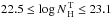 (right panel of Fig. 6), with no overlap with the values of
needed by the slope. We obtained intercepts that are consistent with the observations for
(right panel of Fig. 6), with no overlap with the values of
needed by the slope. We obtained intercepts that are consistent with the observations for
 and
and  for
the relation of Hasinger (2008) and Burlon et al. (2011), respectively. Thus only the hard
X-ray θOA − LX relationship of
Burlon et al. (2011) is able to explain (for
) at
the same time both the intercept and the slope of the X-ray Baldwin effect at high
luminosities.
for
the relation of Hasinger (2008) and Burlon et al. (2011), respectively. Thus only the hard
X-ray θOA − LX relationship of
Burlon et al. (2011) is able to explain (for
) at
the same time both the intercept and the slope of the X-ray Baldwin effect at high
luminosities.
4. Discussion
Since its discovery about 20 years ago, the existence of the X-ray Baldwin effect has been confirmed by several works performed with the highest spectral resolution available in the X-ray band. So far, several explanations have been proposed. Jiang et al. (2006) argued that the observed anti-correlation could be related to the delay of the reprocessed radiation with respect to the primary continuum. The response of the circumnuclear material to the irradiated flux is not simultaneous, and one should always take this effect into account when performing studies of reprocessed features such as the iron Kα line or the Compton hump. Shu et al. (2010, 2012) have shown that averaging the values of LX and EW for all the observations of each source results in a significantly flattened anti-correlation. However, by itself variability fails to fully account for the observed correlation (Shu et al. 2012).
4.1. Explaining the X-ray Baldwin effect with a luminosity-dependent covering factor of the torus
A mechanism often invoked to explain the X-ray Baldwin effect is the decrease of the
covering factor of the molecular torus with the luminosity (e.g., Page et al. 2004; Bianchi et al.
2007). The decrease of the fraction of obscured sources with the luminosity has
been reported by several works performed at different wavelengths in the last decade,
although some discordant results have been presented (e.g., Dwelly & Page 2006; Lawrence
& Elvis 2010). In this work, we have shown that the covering
factor–luminosity relationships obtained in the medium and hard X-ray band can explain
well the X-ray Baldwin effect in the 1042−1044.2 erg s luminosity
range. In particular, our simulations show that it is possible to reproduce the slope of
the X-ray Baldwin effect with luminosity-dependent unification for average equatorial
column densities of the torus of  , and
both the slope and the intercept for (Fig. 5). In the same luminosity range, the
θOA − LX IR relationship of
Maiolino et al. (2007) can explain the X-ray
Baldwin effect for
, and
both the slope and the intercept for (Fig. 5). In the same luminosity range, the
θOA − LX IR relationship of
Maiolino et al. (2007) can explain the X-ray
Baldwin effect for  .
.
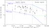 |
Fig. 7 Iron Kα EW versus X-ray luminosities and predicted trends obtained
for different values of the equatorial column density of the torus. The points are
the values of the EW of the iron Kα line reported by Shu et al. (2010) and obtained by averaging
multiple Chandra/HEG observations of AGN. The two blue dash-dotted
lines are the fits to our simulations of the X-ray Baldwin effect using the
θOA − LX relationship of
Hasinger (2008) for the Seyfert regime
(log EW = 1.01−0.17log LX,44
for |
In the quasar regime, we have shown that, while the medium X-ray
θOA − LX relationship of Hasinger (2008) cannot explain the observations
(Fig. 6), the slope obtained by the
IR θOA − LX relationship is
consistent with our fit to the Chandra/HEG data in the same luminosity
band. However, as for the latter relationship, because the range of values of
required to explain the slope and the intercept do not overlap, it cannot be considered a
likely explanation. The hard X-ray
θOA − LX relationship of Burlon et al. (2011) is flat above
 , and would
thus produce a constant EW of the iron Kα line and a slope of
B ~ 0 for the whole range of ,
consistent within 1σ with the value found using
Chandra/HEG data. The intercept we found using this relation is also
consistent with the observational value for a large range of average equatorial column
densities of the torus ().
The fraction of obscured AGN is not well constrained at high luminosities, thus any trend
with the luminosity between that of Burlon et al.
(2011) and that of Hasinger (2008) would
be able to reproduce the observed slope. Because the relation of Hasinger (2008) produces negative values of
f obs for log LX ≳ 45.8, a
flattening of the decline is expected below this luminosity. From Fig. 7 (left panel) in
Hasinger (2008), one can see that above
log LX ≃ 45 the value of f obs
appears to be constant, similarly to what has been found in the hard X-ray band. A
flattening of fobs in the quasar regime would also be expected
when considering the large amount of accreting material needed to power the AGN at these
luminosities. It must, however, be stressed that the X-ray Baldwin effect has not been
well studied at high luminosities, and that the Chandra/HEG sample we
used in this luminosity range is small, not allowing us to reach a firm conclusion on the
variation of the iron Kα EW with the luminosity. Possible evidence of a
flattening of the X-ray Baldwin effect in the quasar regime has recently been found by
Krumpe et al. (2010).
, and would
thus produce a constant EW of the iron Kα line and a slope of
B ~ 0 for the whole range of ,
consistent within 1σ with the value found using
Chandra/HEG data. The intercept we found using this relation is also
consistent with the observational value for a large range of average equatorial column
densities of the torus ().
The fraction of obscured AGN is not well constrained at high luminosities, thus any trend
with the luminosity between that of Burlon et al.
(2011) and that of Hasinger (2008) would
be able to reproduce the observed slope. Because the relation of Hasinger (2008) produces negative values of
f obs for log LX ≳ 45.8, a
flattening of the decline is expected below this luminosity. From Fig. 7 (left panel) in
Hasinger (2008), one can see that above
log LX ≃ 45 the value of f obs
appears to be constant, similarly to what has been found in the hard X-ray band. A
flattening of fobs in the quasar regime would also be expected
when considering the large amount of accreting material needed to power the AGN at these
luminosities. It must, however, be stressed that the X-ray Baldwin effect has not been
well studied at high luminosities, and that the Chandra/HEG sample we
used in this luminosity range is small, not allowing us to reach a firm conclusion on the
variation of the iron Kα EW with the luminosity. Possible evidence of a
flattening of the X-ray Baldwin effect in the quasar regime has recently been found by
Krumpe et al. (2010).
4.2. The differences between X-ray and IR half-opening angle-luminosity relationships
The main difference between the different
θOA − LX relationships that we
used is that those obtained in the X-rays are based on direct observations of the
absorbing material in the line of sight, while the relationship of Maiolino et al. (2007) is extrapolated from the ratio of the thermal
infrared emission to the primary AGN continuum. The
θOA − Lλ(5100 Å)
relationship obtained by Maiolino et al. (2007) was
converted into θOA − LX using the
L 2 keV − Lλ(2500 Å) relation obtained
by Steffen et al. (2006). It was then converted
into the
LX − Lλ(5100 Å)
relation assuming the optical-UV spectral slope obtained by Vanden Berk et al. (2001). All this is likely to introduce some error
in the θOA − LX obtained by their
IR work. It has been argued by Maiolino et al.
(2007) that the larger normalization of the
θOA − LX relation they found is
related to the fact that medium X-ray surveys such as that of Hasinger (2008) are likely to miss a certain fraction of heavily
obscured objects, which can instead be detected in the IR. This is because most of the
X-ray emission is depleted for Compton-thick AGN at energies ≲10 keV. However, hard
X-ray surveys such as that of Burlon et al. (2011),
which are much less biased by absorption, have found a normalization of the
θOA − LX relation consistent
with that obtained at lower X-ray energies (see Fig. 1). Our results also show that the X-ray Baldwin effect can be explained by a
Compton-thin torus and that larger values of fobs would imply
even lower average values of .
Consequently missing heavily obscured objects would not significantly affect our results.
X-rays are also probably better suited to probe the material responsible for the iron
Kα line emission. The line can, in fact, be emitted by both gas and
dust, and while the IR can probe only the latter, X-rays are able to infer the amount of
both gas and dust. We thus conclude that for the purpose of our study the X-ray
θOA − LX relations are better
suited than those extrapolated from IR observations.
It could be argued that the value of the hydrogen column density commonly used to
determine the fraction of obscured objects (and thus as an indicator of the presence of
the torus) is N H ~ 1022 cm, while the torus is
believed to have larger values of ,
and that this obscuration might be related to the presence of dust lanes or molecular
structures in the host galaxy (e.g., Matt 2000).
However, Bianchi et al. (2009), using the results of
Della Ceca et al. (2008), have shown that a
similar decrease of fobs with the luminosity is obtained when
this threshold is set to a larger value of line-of-sight column density. They found that
the fraction of CT AGN decreases with the luminosity as
fCT ∝ L-0.22, similarly to what
is found for fobs in the X-rays (e.g., Hasinger 2008, see Eq. (1)). A similar result was obtained by Fiore
et al. (2009) from a Chandra and Spitzer study
of AGN in the COSMOS field. This implies that the contribution of dust lanes or galactic
molecular structures to the observed N H does not
significantly affect the fobs − LX
relationships obtained in the X-rays.
4.3. The equatorial column density of the torus
The distribution of values of the equatorial column density of the torus in AGN is still
poorly constrained. X-ray observation can in fact infer solely the obscuration in the line
of sight, and only studies of the reprocessed X-ray emission performed using physical
torus models like those of Ikeda et al. (2009),
Brightman & Nandra (2011) and Murphy & Yaqoob (2009) can help to deduce the
value of the equatorial column density of the torus. However, these kinds of studies are
still very scarce (e.g., Rivers et al. 2011; Brightman & Ueda 2012), besides being largely
geometry dependent. Studies of AGN in the mid-IR band performed using the clumpy torus
formalism of Nenkova et al. (2008) have shown that
the number of clouds along the equator is N0 ~ 5−10 (Mor et al. 2009). If, as reported by Mor et al. (2009), each cloud of the torus has an
optical depth of τV ~ 30−100 (i.e.,
 ), the equatorial column
density of the torus is expected to be
), the equatorial column
density of the torus is expected to be  , in agreement with our
results. However, the value of the intercept of the X-ray Baldwin effect obtained by the
simulations is strongly dependent on our assumptions on the metallicity of the torus. This
implies that our constraints of the average value of
are also tightly related to the choice of the metallicity: lower values of the metallicity
would lead to larger values of .
To study this effect, we repeated our study in the Seyfert regime using half-solar
metallicities for the reflection model. We found that in this scenario one needs values of
the equatorial column density of the torus about two times larger than for the
solar-metallicity case (
, in agreement with our
results. However, the value of the intercept of the X-ray Baldwin effect obtained by the
simulations is strongly dependent on our assumptions on the metallicity of the torus. This
implies that our constraints of the average value of
are also tightly related to the choice of the metallicity: lower values of the metallicity
would lead to larger values of .
To study this effect, we repeated our study in the Seyfert regime using half-solar
metallicities for the reflection model. We found that in this scenario one needs values of
the equatorial column density of the torus about two times larger than for the
solar-metallicity case ( ) to
explain the X-ray Baldwin effect. To have a Compton-thick torus, one would then need
values of the metallicity of
Z ≲ 0.2 Z⊙. A Compton-thick torus
has often been invoked to explain the Compton hump observed in the spectrum of many
unobscured AGN (e.g., Bianchi et al. 2004). It is
still unclear, however, which fraction of the Compton hump is produced in the distant
reflector and which in the accretion flow. From our study, we have found that in
unobscured objects the X-ray Baldwin effect can be explained by a luminosity-dependent
covering factor of the torus for an average value of the equatorial column density of
. This value is lower than
the line-of-sight N H of many Seyfert 2s (e.g., Ricci et al. 2011; Burlon et al. 2011) and might be related either to the geometry we adopted or to
the presence of objects with sub-solar metallicities. In particular, due to the constant
reflection angle relative to a local normal in any point of the reflecting surface, the
spherical-toroidal geometry produces larger values of EW (and thus larger values of the
intercept) with respect to a toroidal structure (Murphy
& Yaqoob 2009).
) to
explain the X-ray Baldwin effect. To have a Compton-thick torus, one would then need
values of the metallicity of
Z ≲ 0.2 Z⊙. A Compton-thick torus
has often been invoked to explain the Compton hump observed in the spectrum of many
unobscured AGN (e.g., Bianchi et al. 2004). It is
still unclear, however, which fraction of the Compton hump is produced in the distant
reflector and which in the accretion flow. From our study, we have found that in
unobscured objects the X-ray Baldwin effect can be explained by a luminosity-dependent
covering factor of the torus for an average value of the equatorial column density of
. This value is lower than
the line-of-sight N H of many Seyfert 2s (e.g., Ricci et al. 2011; Burlon et al. 2011) and might be related either to the geometry we adopted or to
the presence of objects with sub-solar metallicities. In particular, due to the constant
reflection angle relative to a local normal in any point of the reflecting surface, the
spherical-toroidal geometry produces larger values of EW (and thus larger values of the
intercept) with respect to a toroidal structure (Murphy
& Yaqoob 2009).
It is possible that there exists a wide spread of equatorial column densities of the
torus in AGN. Thus one could envisage that this, together with the different values of
θ i, would introduce the scatter observed in the
anti-correlation. In Fig. 7 we show the X-ray Baldwin
effect obtained from our simulations using the relationship of Hasinger (2008) for  and
and
 in both the Seyfert and the
quasar regime, together with the time-averaged Chandra/HEG data of Shu et al. (2010). From the figure it is evident that
all the data are well within the range expected from our simulations, both in the Seyfert
and in the quasar regime. It is not known whether there exists a relation between the
equatorial column density of the torus and the AGN luminosity. However, we have shown that
the variation of the covering factor of the torus with the luminosity alone can fully
explain the observed trend, so that no additional luminosity-dependent physical parameter
is needed.
in both the Seyfert and the
quasar regime, together with the time-averaged Chandra/HEG data of Shu et al. (2010). From the figure it is evident that
all the data are well within the range expected from our simulations, both in the Seyfert
and in the quasar regime. It is not known whether there exists a relation between the
equatorial column density of the torus and the AGN luminosity. However, we have shown that
the variation of the covering factor of the torus with the luminosity alone can fully
explain the observed trend, so that no additional luminosity-dependent physical parameter
is needed.
4.4. Luminosity-dependent unification of AGN
The relation of fobs with the luminosity might be connected
to the increase of the inner radius of the torus with the luminosity due to dust
sublimation. Both near-IR reverberation (Suganuma et al.
2006) and mid-IR interferometric (Tristram
& Schartmann 2011) studies have confirmed that the inner radius of the
molecular torus increases with the luminosity as
Rin ∝ L0.5. Considering the
geometry of Fig. 1, the fraction of obscured objects
(see Eq. (4)) would be related to the ratio
of the height to the inner radius of the torus
(H/R) by
 (6)For
values of H/R ≲ 1,
fobs ∝ H/R.
In the original formulation of the receding torus model (Lawrence 1991), the height H was
considered to be constant. Assuming that R has the same luminosity
dependence as Rin, this would lead to
fobs ∝ L-0.5. This has been
shown to be inconsistent with recent observations, which point towards a flatter slope
(fobs ∝ L-0.25, e.g., Hasinger 2008, see Eq. (1)) and imply H ∝ L0.25.
Hönig & Beckert (2007) have shown that in
the frame of the radiation-limited clumpy dust torus model, one would
obtain H ∝ L0.25, which is in agreement with
the observations.
(6)For
values of H/R ≲ 1,
fobs ∝ H/R.
In the original formulation of the receding torus model (Lawrence 1991), the height H was
considered to be constant. Assuming that R has the same luminosity
dependence as Rin, this would lead to
fobs ∝ L-0.5. This has been
shown to be inconsistent with recent observations, which point towards a flatter slope
(fobs ∝ L-0.25, e.g., Hasinger 2008, see Eq. (1)) and imply H ∝ L0.25.
Hönig & Beckert (2007) have shown that in
the frame of the radiation-limited clumpy dust torus model, one would
obtain H ∝ L0.25, which is in agreement with
the observations.
The decrease of the covering factor with luminosity might also have important implications on the AGN dichotomy. It has been shown that Seyfert 2 s appear to have on average lower luminosities and lower Eddington ratios (e.g., Beckmann et al. 2009; Ricci et al. 2011) than Seyfert 1 s and Seyfert 1.5 s, which suggests that they have on average a torus with a larger covering factor. This idea is also supported both by the fact that the luminosity function of type II AGN has been found to peak at lower luminosities than that of type I AGN (Della Ceca et al. 2008; Burlon et al. 2011) and by the results obtained by the recent mid-IR work of Ramos Almeida et al. (2011, see also Elitzur 2012). A difference in the torus covering factor distribution between different types of AGN would also explain why the average hard X-ray spectrum of Compton-thin Seyfert 2s shows a larger reflection component than that of Seyfert 1 s and Seyfert 1.5 s (Ricci et al. 2011). A similar result was found by Brightman & Ueda (2012): studying high-redshift AGN in the Chandra Deep Field South, they found that more obscured objects appear to have tori with larger covering factors, although they did not find a clear luminosity dependence.
5. Summary and conclusions
In this work we have studied the hypothesis that the X-ray Baldwin effect is related to the
decrease of the covering factor of the torus with the luminosity. We used the physical torus
models of Ikeda et al. (2009) and Brightman & Nandra (2011) to account for the
reprocessed X-ray radiation, and the values of the fraction of obscured sources obtained by
recent surveys in the X-rays and in the IR as a proxy of the covering factor of the torus.
Our simulations show that the variation of the covering factor of the torus with the
luminosity can explain the X-ray Baldwin effect. In the Seyfert regime
(LX ≤ 1044.2 erg s-1), the observed
EW − LX trend can be exactly (both in slope
and intercept) reproduced by an average value of the equatorial column density of the torus
of , while a slope consistent with
the observations is obtained for a larger range of column densities
(). At higher luminosities
(LX > 1044.2 erg s-1),
the situation is less clear due to the small number of high-quality observations available.
Moreover, it is not clear whether fobs still decreases with the
luminosity in the quasar regime, similarly to what is found in the Seyfert regime (as shown
by Hasinger 2008), or whether it is constant (as
found by Burlon et al. 2011). A flattening of the
θOA − LX relationship could
explain the observations at high luminosities (for ), and
it might naturally arise from the large amount of accreting mass needed to power these
luminous quasars.
In the next few years ASTRO-H (Takahashi et al. 2010), with its high energy-resolution calorimeter SXS, will allow to constrain the origin of the narrow component of the iron Kα line, being able to separate the narrow core coming from the torus from the flux emitted closer to the central engine even better than Chandra/HEG. ASTRO-H will also be able to probe the narrow iron Kα line in the quasar regime, which will allow us to understand the behavior of the X-ray Baldwin effect at high luminosities.
Acknowledgments
We thank the anonymous referee for his/her comments that helped improve the paper. We thank XinWen Shu and Rivay Mor for providing us with useful details about their work, and Chin Shin Chang and Poshak Gandhi for their comments on the manuscript. C.R. thanks the Sherpa group and IPAG for their hospitality during his stay in Grenoble. C.R. is a Fellow of the Japan Society for the Promotion of Science (JSPS).
References
- Arnaud, K. A. 1996, in Astronomical Data Analysis Software and Systems V, eds. G. H. Jacoby, & J. Barnes, ASP Conf. Ser., 101, 17 [Google Scholar]
- Baldwin, J. A. 1977, ApJ, 214, 679 [NASA ADS] [CrossRef] [Google Scholar]
- Beckmann, V., Soldi, S., Ricci, C., et al. 2009, A&A, 505, 417 [NASA ADS] [CrossRef] [EDP Sciences] [Google Scholar]
- Bianchi, S., Matt, G., Balestra, I., Guainazzi, M., & Perola, G. C. 2004, A&A, 422, 65 [NASA ADS] [CrossRef] [EDP Sciences] [Google Scholar]
- Bianchi, S., Guainazzi, M., Matt, G., & Fonseca Bonilla, N. 2007, A&A, 467, L19 [NASA ADS] [CrossRef] [EDP Sciences] [Google Scholar]
- Bianchi, S., La Franca, F., Matt, G., et al. 2008, MNRAS, 389, L52 [NASA ADS] [Google Scholar]
- Bianchi, S., Bonilla, N. F., Guainazzi, M., Matt, G., & Ponti, G. 2009, A&A, 501, 915 [NASA ADS] [CrossRef] [EDP Sciences] [Google Scholar]
- Brightman, M., & Nandra, K. 2011, MNRAS, 413, 1206 [CrossRef] [Google Scholar]
- Brightman, M., & Ueda, Y. 2012, MNRAS, 2850 [Google Scholar]
- Burlon, D., Ajello, M., Greiner, J., et al. 2011, ApJ, 728, 58 [NASA ADS] [CrossRef] [Google Scholar]
- Croom, S. M., Rhook, K., Corbett, E. A., et al. 2002, MNRAS, 337, 275 [NASA ADS] [CrossRef] [Google Scholar]
- de La Cal le Pérez, I., Longinotti, A. L., Guainazzi, M., et al. 2010, A&A, 524, A50 [NASA ADS] [CrossRef] [EDP Sciences] [Google Scholar]
- Della Ceca, R., Caccianiga, A., Severgnini, P., et al. 2008, A&A, 487, 119 [NASA ADS] [CrossRef] [EDP Sciences] [Google Scholar]
- Dietrich, M., Hamann, F., Shields, J. C., et al. 2002, ApJ, 581, 912 [NASA ADS] [CrossRef] [Google Scholar]
- Dwelly, T., & Page, M. J. 2006, MNRAS, 372, 1755 [NASA ADS] [CrossRef] [Google Scholar]
- Elitzur, M. 2012, ApJ, 747, L33 [NASA ADS] [CrossRef] [Google Scholar]
- Elitzur, M., & Shlosman, I. 2006, ApJ, 648, L101 [NASA ADS] [CrossRef] [Google Scholar]
- Fabian, A. C., Iwasawa, K., Reynolds, C. S., & Young, A. J. 2000, PASP, 112, 1145 [NASA ADS] [CrossRef] [Google Scholar]
- Fiore, F., Puccetti, S., Brusa, M., et al. 2009, ApJ, 693, 447 [NASA ADS] [CrossRef] [Google Scholar]
- Fukazawa, Y., Hiragi, K., Mizuno, M., et al. 2011, ApJ, 727, 19 [NASA ADS] [CrossRef] [Google Scholar]
- Gandhi, P., Horst, H., Smette, A., et al. 2009, A&A, 502, 457 [NASA ADS] [CrossRef] [EDP Sciences] [Google Scholar]
- Grandi, P., Malaguti, G., & Fiocchi, M. 2006, ApJ, 642, 113 [NASA ADS] [CrossRef] [Google Scholar]
- Green, P. J., Forster, K., & Kuraszkiewicz, J. 2001, ApJ, 556, 727 [NASA ADS] [CrossRef] [Google Scholar]
- Grimes, J. A., Rawlings, S., & Willott, C. J. 2004, MNRAS, 349, 503 [NASA ADS] [CrossRef] [Google Scholar]
- Hasinger, G. 2008, A&A, 490, 905 [NASA ADS] [CrossRef] [EDP Sciences] [Google Scholar]
- Hönig, S. F., & Beckert, T. 2007, MNRAS, 380, 1172 [NASA ADS] [CrossRef] [Google Scholar]
- Hönig, S. F., Smette, A., Beckert, T., et al. 2008, A&A, 485, L21 [NASA ADS] [CrossRef] [EDP Sciences] [Google Scholar]
- Ikeda, S., Awaki, H., & Terashima, Y. 2009, ApJ, 692, 608 [NASA ADS] [CrossRef] [Google Scholar]
- Iwasawa, K., & Taniguchi, Y. 1993, ApJ, 413, L15 [NASA ADS] [CrossRef] [Google Scholar]
- Jiang, P., Wang, J. X., & Wang, T. G. 2006, ApJ, 644, 725 [NASA ADS] [CrossRef] [Google Scholar]
- Jiménez-Bailón, E., Piconcelli, E., Guainazzi, M., et al. 2005, A&A, 435, 449 [NASA ADS] [CrossRef] [EDP Sciences] [Google Scholar]
- Krolik, J. H., Madau, P., & Zycki, P. T. 1994, ApJ, 420, L57 [NASA ADS] [CrossRef] [Google Scholar]
- Krumpe, M., Lamer, G., Markowitz, A., & Corral, A. 2010, ApJ, 725, 2444 [NASA ADS] [CrossRef] [Google Scholar]
- Lawrence, A. 1991, MNRAS, 252, 586 [NASA ADS] [Google Scholar]
- Lawrence, A., & Elvis, M. 1982, ApJ, 256, 410 [NASA ADS] [CrossRef] [Google Scholar]
- Lawrence, A., & Elvis, M. 2010, ApJ, 714, 561 [NASA ADS] [CrossRef] [Google Scholar]
- Magdziarz, P., & Zdziarski, A. A. 1995, MNRAS, 273, 837 [NASA ADS] [CrossRef] [Google Scholar]
- Maiolino, R., Shemmer, O., Imanishi, M., et al. 2007, A&A, 468, 979 [NASA ADS] [CrossRef] [EDP Sciences] [Google Scholar]
- Matt, G. 2000, A&A, 355, L31 [NASA ADS] [Google Scholar]
- Matt, G., Guainazzi, M., & Maiolino, R. 2003, MNRAS, 342, 422 [NASA ADS] [CrossRef] [Google Scholar]
- Miyakawa, T., Ebisawa, K., & Inoue, H. 2012, PASJ, 64, 140 [NASA ADS] [Google Scholar]
- Mor, R., Netzer, H., & Elitzur, M. 2009, ApJ, 705, 298 [NASA ADS] [CrossRef] [Google Scholar]
- Murphy, K. D., & Yaqoob, T. 2009, MNRAS, 397, 1549 [NASA ADS] [CrossRef] [Google Scholar]
- Nandra, K. 2006, MNRAS, 368, L62 [NASA ADS] [CrossRef] [Google Scholar]
- Nandra, K., George, I. M., Mushotzky, R. F., Turner, T. J., & Yaqoob, T. 1997, ApJ, 488, L91 [NASA ADS] [CrossRef] [Google Scholar]
- Nandra, K., O’Neill, P. M., George, I. M., & Reeves, J. N. 2007, MNRAS, 382, 194 [NASA ADS] [CrossRef] [Google Scholar]
- Nenkova, M., Sirocky, M. M., Ivezić, Ž., & Elitzur, M. 2008, ApJ, 685, 147 [NASA ADS] [CrossRef] [Google Scholar]
- Netzer, H., Laor, A., & Gondhalekar, P. M. 1992, MNRAS, 254, 15 [NASA ADS] [CrossRef] [Google Scholar]
- Page, K. L., O’Brien, P. T., Reeves, J. N., & Turner, M. J. L. 2004, MNRAS, 347, 316 [NASA ADS] [CrossRef] [Google Scholar]
- Petrucci, P. O., Henri, G., Maraschi, L., et al. 2002, A&A, 388, L5 [NASA ADS] [CrossRef] [EDP Sciences] [Google Scholar]
- Ramos Almeida, C., Levenson, N. A., Alonso-Herrero, A., et al. 2011, ApJ, 731, 92 [NASA ADS] [CrossRef] [Google Scholar]
- Reeves, J. N., & Turner, M. J. L. 2000, MNRAS, 316, 234 [NASA ADS] [CrossRef] [Google Scholar]
- Ricci, C., Walter, R., Courvoisier, T. J.-L., & Paltani, S. 2011, A&A, 532, A102 [NASA ADS] [CrossRef] [EDP Sciences] [Google Scholar]
- Rivers, E., Markowitz, A., & Rothschild, R. 2011, ApJ, 732, 36 [NASA ADS] [CrossRef] [Google Scholar]
- Shu, X. W., Yaqoob, T., & Wang, J. X. 2010, ApJS, 187, 581 [NASA ADS] [CrossRef] [Google Scholar]
- Shu, X. W., Yaqoob, T., & Wang, J. X. 2011, ApJ, 738, 147 [NASA ADS] [CrossRef] [Google Scholar]
- Shu, X. W., Wang, J. X., Yaqoob, T., Jiang, P., & Zhou, Y. Y. 2012, ApJ, 744, L21 [NASA ADS] [CrossRef] [Google Scholar]
- Simpson, C. 2005, MNRAS, 360, 565 [NASA ADS] [CrossRef] [Google Scholar]
- Singh, V., Shastri, P., & Risaliti, G. 2011, A&A, 532, A84 [NASA ADS] [CrossRef] [EDP Sciences] [Google Scholar]
- Steffen, A. T., Strateva, I., Brandt, W. N., et al. 2006, AJ, 131, 2826 [NASA ADS] [CrossRef] [Google Scholar]
- Suganuma, M., Yoshii, Y., Kobayashi, Y., et al. 2006, ApJ, 639, 46 [NASA ADS] [CrossRef] [Google Scholar]
- Takahashi, T., Mitsuda, K., Kelley, R., et al. 2010, in SPIE Conf. Ser., 7732 [Google Scholar]
- Treister, E., Krolik, J. H., & Dullemond, C. 2008, ApJ, 679, 140 [NASA ADS] [CrossRef] [Google Scholar]
- Tristram, K. R. W., & Schartmann, M. 2011, A&A, 531, A99 [NASA ADS] [CrossRef] [EDP Sciences] [Google Scholar]
- Turner, T. J., & Miller, L. 2009, A&ARv, 17, 47 [Google Scholar]
- Ueda, Y., Akiyama, M., Ohta, K., & Miyaji, T. 2003, ApJ, 598, 886 [NASA ADS] [CrossRef] [Google Scholar]
- Ueda, Y., Hiroi, K., Isobe, N., et al. 2011, PASJ, 63, 937 [Google Scholar]
- Van den Berk, D. E., Richards, G. T., Bauer, A., et al. 2001, AJ, 122, 549 [NASA ADS] [CrossRef] [Google Scholar]
- Yaqoob, T., & Padmanabhan, U. 2004, ApJ, 604, 63 [NASA ADS] [CrossRef] [Google Scholar]
- Zhou, X.-L., & Wang, J.-M. 2005, ApJ, 618, L83 [NASA ADS] [CrossRef] [Google Scholar]
All Tables
Summary of the most recent studies (along with the original work of Iwasawa & Taniguchi 1993) of the X-ray Baldwin effect.
All Figures
|
Fig. 1 Schematic representation of the torus geometry considered. The angle
θ i is the inclination of the line of sight with
respect to the torus axis, while θOA and
|
| In the text | |
|
Fig. 2 Variation of the fraction of obscured sources (fobs) and of the half-opening angle of the torus (θOA) with the 2–10 keV luminosity for three of the most recent medium X-ray (2–10 keV, Hasinger 2008), hard X-ray (15–55 keV, Burlon et al. 2011), and IR (Maiolino et al. 2007) studies (Eqs. (1)–(3)). |
| In the text | |
|
Fig. 3 Top panel: extract in the 5.5–7.5 keV region of a spectrum
simulated using the model of Ikeda et al.
(2009). The model has a torus with a half-opening angle of
θOA = 46.2° (equivalent to
log LX = 42.7, according to the relationship of Hasinger 2008), an equatorial column density of
|
| In the text | |
|
Fig. 4 Equivalent width of the iron Kα line versus the X-ray luminosity
obtained simulating a torus with an equatorial column density of
|
| In the text | |
|
Fig. 5 Left panel: value of the slope (B) of the X-ray
Baldwin effect obtained simulating the variation of the reprocessed X-ray radiation
with the luminosity for tori with different values of the equatorial column density
|
| In the text | |
|
Fig. 6 Left panel: value of the slope (B) of the X-ray
Baldwin effect obtained simulating the variation of the reprocessed X-ray radiation
with the luminosity for tori with different values of the equatorial column density
|
| In the text | |
|
Fig. 7 Iron Kα EW versus X-ray luminosities and predicted trends obtained
for different values of the equatorial column density of the torus. The points are
the values of the EW of the iron Kα line reported by Shu et al. (2010) and obtained by averaging
multiple Chandra/HEG observations of AGN. The two blue dash-dotted
lines are the fits to our simulations of the X-ray Baldwin effect using the
θOA − LX relationship of
Hasinger (2008) for the Seyfert regime
(log EW = 1.01−0.17log LX,44
for |
| In the text | |
Current usage metrics show cumulative count of Article Views (full-text article views including HTML views, PDF and ePub downloads, according to the available data) and Abstracts Views on Vision4Press platform.
Data correspond to usage on the plateform after 2015. The current usage metrics is available 48-96 hours after online publication and is updated daily on week days.
Initial download of the metrics may take a while.