| Issue |
A&A
Volume 552, April 2013
|
|
|---|---|---|
| Article Number | A47 | |
| Number of page(s) | 23 | |
| Section | Astronomical instrumentation | |
| DOI | https://doi.org/10.1051/0004-6361/201220408 | |
| Published online | 21 March 2013 | |
Cross-calibration of Suzaku/XIS and XMM-Newton/EPIC using galaxy clusters
1
Department of PhysicsUniversity of Helsinki,
Dynamicum, PO Box 48
00014
Helsinki,
Finland
e-mail:
kimmo.kettula@iki.fi
2
Finnish Centre for Astronomy with ESO, University of
Turku, Väisäläntie
20, 21500
Piikkiö,
Finland
e-mail:
jukka.h.nevalainen@helsinki.fi
3
Tartu Observatory, 61602
Tõravere,
Estonia
4
Kavli Institute for Astrophysics and Space Research, Massachusetts
Institute of Technology, 77
Massachusetts Avenue, Cambridge, MA
02139,
USA
Received: 19 September 2012
Accepted: 11 January 2013
Aims. We extend a previous cross-calibration study conducted by the International Astronomical Consortium for High Energy Calibration (IACHEC) on XMM-Newton/EPIC, Chandra/ACIS and BeppoSAX/MECS X-ray instruments with galaxy clusters to Suzaku/XIS instruments. Our aim is to study the accuracy of the energy-dependent effective area calibration of the XIS instruments using observations during 2005–2008.
Methods. We performed a spatially resolved X-ray spectral analysis on Suzaku/XIS and XMM-Newton/EPIC-pn data for a sample of galaxy clusters. We extracted spectra from 3–6 arcmin annular regions. By comparing the spectroscopic temperatures, fluxes, and fit residuals obtained with different instruments for the same cluster, we evaluated the systematic uncertainties of the energy dependence and the normalisation of the effective area between different detectors.
Results. The temperatures measured in the hard 2.0–7.0 keV energy band with all instruments are consistent within ~5%. Thus Suzaku/XIS can be added to the previously found list of instruments with good agreement of the effective area shape in the hard band (XMM-Newton/EPIC, Chandra/ACIS and BeppoSAX/MECS). However, using the public calibration, the temperatures obtained with the XIS instruments in the soft 0.5–2.0 keV band disagree by 9–29%. We investigated residuals in the XIS soft band, which showed that if the XIS0 effective area shape is accurately calibrated, the effective areas of XIS1 and XIS3 are overestimated below ~1.0 keV (or vice versa), with the difference increasing to ~20% at 0.5 keV. Adjustments to the modelling of the column density of the XIS contaminant in the 3–6 arcmin extraction region while forcing consistent emission models in each instrument for a given cluster significantly improved the fits. Assuming the composition of the contaminant as in the public calibration, the oxygen column density in the XIS1 and XIS3 contaminants must be increased by ~1–2 × 1017 cm-2 in comparison to the values implemented in the current calibration, while the column density of the XIS0 contaminant given by the analysis is consistent with the public calibration. This indicates that the effective area shape of XIS0 in the soft band is more accurately modelled in the public calibration than that of XIS1 and XIS3. XIS soft band temperatures obtained with the modification to the column density of the contaminant agree better with temperatures obtained with the EPIC-pn instrument of XMM-Newton than with those derived using the Chandra/ACIS instrument. However, as the hard band data of the Suzaku/XIS and EPIC-pn instruments yield a maximum systematic uncertainty of 10% on the derived fluxes, comparing the hard band fluxes obtained using Suzaku/XIS to fluxes obtained using the Chandra/ACIS and EPIC-pn instruments proved inconclusive.
Key words: instrumentation: miscellaneous / techniques: spectroscopic / galaxies: clusters: intracluster medium / X-rays: galaxies: clusters
© ESO, 2013
1. Introduction
Clusters of galaxies are bright, stable, and extended objects, which makes them suitable for X-ray calibration. The X-ray spectra of clusters typically consist of a combination of thermal bremsstrahlung and collisionally excited line emission. Temperature measurements of clusters above kT ~ 2 keV are dominated by the shape of the X-ray continuum. Consequently, by comparing temperatures of the same cluster measured with different instruments, one can gain an indication on the cross-calibration status of the energy dependence of the effective area (defined here as the product of the mirror effective area, detector quantum efficiency and filter transmission) between the instruments. Similarly, the normalisation of the effective area affects the determination emission measure and cluster flux, and comparing cluster fluxes measured with different instruments accordingly yields information about the relative normalisation of the effective areas of the instruments. Analysis of the residuals of the spectral fits yields more detailed information on the cross-calibration.
The International Astronomical Consortium for High Energy Calibration (IACHEC)1 was formed to provide standards for high-energy calibration and to supervise cross-calibration between different observatories. This paper is based on the activities of the IACHEC clusters working group. The working group performed a study of galaxy clusters to investigate the effective area cross-calibration status between the XMM-Newton/EPIC, Chandra/ACIS and BeppoSAX/MECS instruments (Nevalainen et al. 2010). They found that while the energy dependence of the effective area is accurately calibrated in the hard energy band (2.0–7.0 keV), the effective area normalisations disagree by 5–10%. They also found significant cross-calibration differences in the soft energy band (0.5–2.0 keV). They determined that temperatures measured with Chandra/ACIS are systematically ~20% higher than those measured with XMM-Newton/ EPIC instruments. This amounts to a ~10% uncertainty of the ACIS and EPIC soft band cross-calibration of the effective area energy dependence. Due to the high statistical weight of the soft band data, Nevalainen et al. (2010) estimated that Chandra/ACIS and XMM-Newton/EPIC cluster temperatures measured in a typical 0.5–7.0 keV energy band suffer from a systematic uncertainty of 10–15% due to the cross-calibration uncertainties.
We extend the IACHEC cluster work to include Suzaku/XIS (Koyama et al. 2007). We evaluated the cross-calibration accuracy of the XIS instruments by comparing measured temperatures and spectral fit residuals. By comparing the measurements with XIS and EPIC-pn (Strüder et al. 2001) we aim to improve the knowledge about the soft band cross-calibration uncertainty between EPIC and ACIS2.
This paper is organised as follows. In Sect. 2 we present the cluster sample used for our study, and in Sect. 3 we discuss the selected spectral extraction regions. We present data reduction and background modelling methods in Sects. 4 and 5. We discuss the spectral analysis method in Sect. 6 and present the results from the analysis in Sects. 7 and 8. In Sect. 9, we investigate if uncertainties in the calibration of the optical blocking filter (OBF) molecular contaminant may affect the cross-calibration of the effective area energy dependence. Finally, we present our concluding remarks in Sect. 10. Throughout this paper, we use 68% (1σ) confidence level for errors, unless stated otherwise.
2. Cluster sample
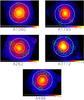 |
Fig. 1 XIS1 raw count rate maps (not corrected for background or vignetting) of the soft band cluster sample in a 0.5–7.0 keV energy band binned to 8 pixels (~0.14 arcmin) per bin. The inner and outer radii of the 3–6 arcmin extraction region are denoted by white circles, the green circles show the excluded regions centred on point sources seen in XMM-Newton/EPIC-pn images. Scaling of the maps is adjusted for clarity and does not reflect the relative brightness of the clusters. The colour bar shows the the total number of counts per bin. |
We constructed a cluster sample consisting of the Highest X-ray Flux Galaxy Cluster Sample (HIFLUGCS) clusters (Reiprich & Böhringer 2002) with XMM-Newton and Suzaku observations that were publicly available in June 2011, using the selection criteria detailed below. The clusters passing our selection criteria (see below) have been observed during the years 2005–2008 (Suzaku) and 2000–2009 (XMM-Newton). The chosen clusters are all bright (flux ~10-12–10-10 erg/cm2/s in a 2–7 keV band) and nearby (z ≤ 0.0753). General properties of the cluster sample are presented in Tables 1 and 2.
General information on the cluster sample.
General information on the observations of the sample.
We only selected pointings where the off-axis angle between the cluster centre and the field of view (FOV) centre is smaller than 1 arcmin. This ensures that we are studying the same detector regions and thus do not fold in any additional calibration uncertainties that depend on the position of the detector.
We performed spectral analysis in two energy bands: 0.5–2.0 keV (soft band) and 2.0–7.0 keV (hard band). We required that the observations have a minimum of 5000 and a maximum of 500 000 data counts in the soft and hard energy bands. The lower limit ensures a sufficient number of counts to obtain reliable statistics, while the upper limit eliminates high signal-to-noise data in which other calibration uncertainties, such as gain and energy redistribution, are significant. We also excluded clusters whose total sky and non X-ray background exceeded 10% of the cluster flux (see Sect. 5 for details on background modelling).
To minimise additional uncertainties in the soft energy band, we excluded clusters with a galactic absorption column density NH > 6 × 1020 cm-2 from the soft band sample (see Table 3). Thus the soft band sample contains a smaller number of objects than the hard band sample.
Properties of the observations.
3. Extraction regions
Because we attempted to minimise point spread function (PSF) scatter and background contamination, we chose to use 3–6 arcmin annuli around the cluster centres as extraction regions (see Fig. 1). By excluding the inner 3 arcmin we minimise the Suzaku PSF scatter from the cool core (see Sect. 5.5). The width of the annulus is larger than the Suzaku PSF so that the PSF scatter to and from the extraction region is minimised. By excluding the regions outside 6 arcmin distance from the cluster centre, i.e. remaining in the bright central regions, we minimise the effect of background contamination.
The useful detector area (when excluding the CCD gaps and the regions around the calibration sources) varies somewhat between different XIS instruments. The fraction of the full extraction annuli covered by the useful detector area varies at most by 12% between the different instruments. We therefore assume that the temperature measurements are not significantly affected by the difference in the covered regions.
4. Data reduction
The general properties of the observations are listed in Table 2.
4.1. Suzaku
We used HEASoft3 release 6.11, containing Suzaku ftools version 18, for the processing. XIS calibration information was from XIS CALDB release 201106084 and XRT calibration information from XRT CALDB release 200807095.
We used the aepipeline tool to reprocess and screen the data and the xselect tool to extract spectra, images, and light curves. We used standard filtering, with the exception that we eliminated times with geomagnetic cut-off rigidity (COR2) less than 6 and time since the South Atlantic Anomaly (SAA) passage less than 436 s. We excluded regions contaminated by the 55Fe calibration sources and circular regions with a radius of 1 arcmin centred on bright point sources seen in XMM-Newton images (see Fig. 1).
We constructed the energy redistribution files with the xisrmfgen and auxiliary response files with the xissimarfgen tool. For each cluster, we used the XMM-Newton/EPIC-pn count rate map to weight the position-dependent effective area with the brightness distribution when producing the auxiliary responses. For the sky background modelling we produced the auxiliary responses assuming a circular source of uniform brightness with a radius of 20 arcmin. We used makepi files version 20070124 and 20100929, RMF parameter file version 20080901 and contamination file version 20091201 as included in XIS CALDB release 20110608.
We checked the XIS1 gain by searching for residuals in the spectral fits (Sect. 6) around the Fe xxv lines. We found evidence for residuals in the Centaurus cluster and performed a gain fit in Xspec. However, the cluster temperature was unaffected.
4.2. XMM-Newton/EPIC-pn
We reduced the EPIC-pn data with SAS version xmmsas_20110223_1801-11.0.0 and the latest calibration information available in June 2011 and produced event files with the epchain tool with the default parameters. We filtered the event files, excluding bad pixels and CCD gaps (i.e. using expression flag = 0), including only patterns 0–4. We generated simulated out-of-time event files, which we used to subtract events registered during CCD readout according to pn mode (Table 2).
We extracted spectra, images, and light curves from the event file with the evselect tool, excluding regions contaminated by bright point sources. We used the light curves to further filter the events by excluding the periods when the E > 10 keV band flux exceeded the quiescent rate by ~20% We produced energy redistribution and auxiliary response files with the rmfgen and arfgen tools. We used the arfgen tool in extended source configuration and weighted the response with an XMM-Newton image of the cluster in detector coordinates, binned in 0.5 arcmin pixels.
5. Background modelling
Because our sample consists of nearby clusters that fill the whole FOV, local estimates for the background emission are not available.
5.1. Sky background
We used the ROSAT All Sky Survey based HEASARC X-ray background tool6 to estimate the spectra of the sky background for both XMM-Newton/EPIC and Suzaku/XIS instruments. We extracted spectra of annular fields centred on the clusters, with an inner radius of 0.5 degrees and outer radius of 1.0 degrees. We fitted the spectra with a model consisting of an absorbed and unabsorbed thermal MEKAL emission component with solar abundances (Mewe et al. 1995), describing emission from the Galactic halo and Local Hot Bubble, and an absorbed power-law with the index fixed to 1.45, describing the extragalactic X-ray background7. We fixed the absorption column densities to the value of the respective clusters (see Sect. 6). We added the local sky background emission model to all subsequent spectral fits. To account for the uncertainty in the sky background model, we allowed the temperatures and normalisations of the emission components to vary within 1.0σ of their best-fit values during subsequent spectral fits.
5.2. XMM-Newton non X-ray background
We extracted and investigated full FOV hard energy band (10–14 keV) EPIC-pn light curves to determine the quiescent non-X-ray background levels and performed GTI filtering by excluding flares. We modelled the quiescent particle background by scaling a sample of closed filter spectra (Nevalainen et al. 2005) to match hard band full FOV spectra. We removed the scaled closed filter spectra from the cluster spectra by using them as correction files is Xspec in subsequent pn spectral fits.
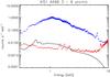 |
Fig. 2 Total emission (blue crosses), sky background (black curve), and non X-ray background (red crosses) emission of A496 in the 3–6 arcmin region for XIS1. The sky background is modelled from ROSAT All Sky Survey data and folded through the XIS1 response. The XIS1 observation of A496 has the strongest relative background emission of the cluster sample. |
We studied the uncertainty of the adopted particle background model by varying the scaling of the closed filter spectra by ±10% and interpreted the change in the best-fit temperature as a systematic effect due to background uncertainties. This had on average a ~3% effect on the best-fit temperatures in the hard band; in the soft band, the effect was less than 0.1% for all clusters in our sample. We propagated this uncertainty by adding it in quadrature to the statistical uncertainties of the temperatures.
5.3. Suzaku non X-ray background
We used the xisnxbgen tool with default settings to generate spectra of the Suzaku/XIS non X-ray background (NXB) based on night Earth observations. We used COR2 weighting for the NXB, construction, and to verify the normalisation of the NXB generated using the xisnxbgen tool, we compared the >10 keV NXB flux with that in the cluster data and found them to be consistent. We subsequently subtracted the NXB spectra from the cluster spectra in all Suzaku/XIS spectral fits by using the NXB spectra as background files in Xspec and thus considered the uncertainty of the NXB in the spectral fits.
5.4. Charge exchange contamination
Geocoronal and heliospheric solar wind charge exchange (SWCX; Wargelin et al. 2004; Snowden et al. 2004; Fujimoto et al. 2007) may contaminate the cluster emission in terms of emission lines in the 0.5–0.9 keV band. The total flux of the SWCX varies by an order of magnitude at a timescale of hours or minutes, reaching a maximum level comparable to that of the sky background (Galactic emission + CXB). To obtain an conservative estimate of the possible SWCX effect on our results, we examined the variation of the best-fit 0.5–2.0 keV energy band temperatures of XIS1 when keeping the sky background model fixed to RASS values, and by increasing the normalisation by 100%. Because of the low level of the sky background compared to the cluster flux in our sample the above effect was insignificant.
5.5. XIS point spread function
Cluster flux originating from a given extraction region may be contaminated by PSF scattered flux from neighbouring regions (e.g. Sato et al. 2007). Since Suzaku/XIS has a relatively large PSF (~2 arcmin half-power diameter), scatter from cool cores may affect the observed XIS temperatures. Therefore we examined how well PSF scatter to and from our extraction region (3–6 arcmin annulus, see Sect. 3) is minimised by extraction regions that are wider and farther away from the centre than the half-power diameter of the XIS PSF.
The exact PSF scattering effects depend on the brightness of the cool centre, the shape of the surface density profile, the temperature of the cluster, and on the cluster redshift, and therefore they can vary from cluster to cluster. We chose to use A1795 and A3112 as conservative examples for the PSF-induced systematic uncertainty, because they possess cool cores that are an order of magnitude brighter than the cores of the rest of the sample (Peres et al. 1998).
We performed ray-tracing simulations of A1795 with xissim to estimate the fraction of photons that originate from the central cool region (r ~ 1.5 arcmin; Vikhlinin et al. 2005) but are scattered into the 3–6 arcmin annulus. We used an exposure-corrected 0.5–7.5 keV energy band XMM-Newton/EPIC-pn rate map of A1795 as a source brightness model and, since the energy dependence of the PSF is known to be weak (e.g. Sato et al. 2007, Appendix 1), we performed the simulation at 1 keV. We accounted for typical pointing errors by using the attitude and exposure information from the Suzaku observations of A1795 used in this work. The simulations show that about 16% of the flux detected in the 3–6 arcmin extraction region originates from the inner 1.5 arcmin cool core. There is a small variation of scattered light between detectors, with values of 13% (XIS0), 18% (XIS1), and 15% (XIS0).
We then simulated a XIS1 spectrum in the 3–6 arcmin annulus containing one MEKAL component for the emission originating from that region and another for the PSF scattered emission from the cool core. We used the Chandra measurements of A1795 (Vikhlinin et al. 2005) for the temperature and abundance of the two components: kT = 6.5 keV, 0.25 solar and kT = 4.75 keV, 0.55 solar, respectively. We used the relative model normalisations of 0.84 and 0.16 given by the above PSF simulations. We fitted the simulated spectrum with a single temperature MEKAL model in the soft 0.5–2.0 keV and hard 2.0–7.0 keV energy bands. The resulting best-fit temperatures were lower by ~7% in the soft band and ~6% in the hard band compared to those obtained from the fits to the observational data.
Lehto et al. (2010) performed an analogous XIS PSF scatter ray-tracing simulation on A3112 data using a 3–6 arcmin extraction region similar to ours. They found that ~10% of the flux in the extraction region originates from the core, but best-fit temperatures were consistent within 2% in all energy bands. The other clusters are weaker (or non-) cool cores, therefore we expect lower biases for all of them. Thus we conclude that cool-core contributions may bias Suzaku/XIS temperatures low, but only up to 6–7% at most, and much less in most cases. However, as the three XIS instruments have similar scattered light properties, they would be biased by similar amounts and the relative XIS temperature differences would be unaffected. Consequently, the effect is only limited to XIS-pn temperature comparisons.
6. Methods
Nevalainen et al. (2010) found that several independent missions/instruments (XMM-Newton/EPIC, Chandra/ACIS, BeppoSAX/MECS) and two independent physical processes (bremsstrahlung and collisionally excited line emission) yielded consistent temperatures in the 2–7 keV band. However, Nevalainen et al. (2010) also found that the 2–7 keV band EPIC/ACIS fluxes disagree by 5–10%. Here we test the above findings with Suzaku/XIS by studying the cross-calibration of the the effective area by spectroscopic analysis of cluster data obtained with Suzaku/XIS instruments and the XMM-Newton/ EPIC-pn instrument.
6.1. Spectral analysis
We extracted spectra of the clusters in our sample from annular 3–6 arcmin regions centred on the clusters (see Sect. 3). We binned the spectra to a minimum of 100 counts per bin. We fitted the NXB-subtracted spectra (see Sects. 5.3 and 5.2) with a model consisting of an absorbed single temperature MEKAL model (Mewe et al. 1995) and the sky background component (see Sect. 5.1). We used metal abundances of Grevesse & Sauval (1998). We modelled the Galactic absorption with the PHABS model, fixing the column densities to the values obtained with 21 cm radio observations (Kalberla et al. 2005) and using the absorption cross sections of Balucinska-Church & McCammon (1992). We allowed the temperature, metal abundance and normalisation of the cluster emission model to vary in the fits. We performed the fits in two energy bands: 0.5–2.0 keV (soft band) and 2.0–7.0 keV (hard band).
In addition to excluding clusters with NH > 6 × 1020 cm2 from the soft band sample (Sect. 2), we excluded Coma from the soft band sample because we were not able to produce single-temperature spectral fits of satisfactory statistical quality. Thus the soft band sample contains fever objects than the hard band sample. The properties of the observations are presented in Table 3.
We experimented with using C statistics (Cash 1979) in addition to standard χ2 statistics to estimate the best-fit parameters. We compared the temperatures obtained by fitting unbinned XIS1 spectra using C statistics to XIS1 temperatures obtained using χ2 statistics and binning the spectra to a minimum of 100 counts per bin. Using the statistical analysis described below, we found that the C statistics yields systematically higher temperatures, with an average temperature difference of 0.5% in the soft 0.5–2.0 keV energy band (statistical significance 0.2σ) and 0.8% in the hard 2.0–7.0 keV energy band (0.8σ). This shows that the choice of statistics in spectral fits can have an impact on cluster temperatures, but it has a low statistical significance and the effect is consequently minimal due to the high number of counts in our spectra. We used binned spectra and χ2 statistics for the remainder of this paper.
6.2. Comparison of temperatures and fluxes
We computed the difference in temperature or flux measurements and their statistical significance for each cluster and instrument pairing in terms of a fraction of the average value, fT = ΔT/ ⟨ T ⟩ = (T1 − T2)/ { (T1 + T2)/2 } and σT = σΔT/ ⟨ T ⟩; fF = ΔF/ ⟨ F ⟩ = (F1 − F2)/ { (F1 + F2)/2 } and σF = σΔF/ ⟨ F ⟩, respectively. Because a systematic uncertainty in calibration would tend to drive the mean of the temperature or flux differences away from zero, we attributed fT or fF as a measure of the relative systematic uncertainty in the cross-calibration of a given instrument pair.
6.3. Stacked residuals
To examine the cross-calibration accuracy of the effective area of the instruments, we applied the stacked-residuals method (Longinotti et al. 2008). This method involves a choice of a reference instrument, against which the other instruments are compared. Since we do not know which, if any, instrument has its effective area perfectly calibrated, the choice of a reference instrument is arbitrary and the comparison is only relative.
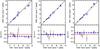 |
Fig. 3 Upper panel: best-fit hard band temperatures (asterisks) and 1σ uncertainties (boxes) for Suzaku/XIS instruments using the public calibration. The solid black line is an identity line, drawn as a reference. Lower panel: relative temperature differences fT (diamonds) between different Suzaku/XIS instruments, and their 1σ uncertainties. The dotted and dashed lines show the weighted means of the relative temperature difference and corresponding uncertainties. |
The stacked residuals method for a pair of instruments, I1 and I2, involves the following steps:
-
We started with the data(dataI1,I2) and responses (respI1,I2), defined here as the energy response matrix (RMF) multiplied with the effective area (ARF), of the instruments. For this example we used I1 as the reference instrument and performed a spectral analysis as explained above for each cluster to fit a reference model (modelI1).
-
To be able to compare the data of different instruments, we regrouped dataI1,I2 to equal binning.
-
For each source, we convolved the reference model with the instrument response to produce an I1-based model prediction (predI1,I2 = modelI1 ⊗ respI1,I2).
-
We divided the data of each cluster by the above model prediction to obtain residuals over the I1-based prediction (residI1,I2 = dataI1,I2/predI1,I2).
-
We divided the above residuals of I2 with I1 residuals, to remove effects of possible calibration uncertainties of I1, obtaining ratio R21 for I2:
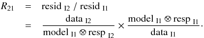 (1)R21 is a useful measure of the effective area cross-calibration, since the value for each energy bin would be unity if the cross-calibration of the I1 and I2 effective areas is consistent.
 -
We calculated the median and median absolute deviation of R21 values for each energy channel for the cluster sample.
7. Results
The best-fit single-temperature models, data, and spectral parameters are shown in Appendix A.
7.1. Hard band
We found that the hard band (2.0–7.0 keV) temperatures measured with XIS0 and XIS3 agree, with an average difference of ~1% (statistical significance 0.7σ). Temperatures measured with XIS1 are on average ~5% (5.6σ) and ~5% (4.9σ) higher than those measured with XIS0 and XIS3 (see Fig. 3).
The simultaneous Suzaku/XMM-Newton observations of BL Lac object PKS2155-304 (Ishida et al. 2011) are useful for comparison with our cluster results since the observations cover the same time period (2005–2008). The XIS CALDB version used by Ishida et al. (2011) for PKS2155-304 (dated July 30, 2010) differs from the one used for our cluster study (dated June 8, 2011) in the model used for the molecular OBF contamination (see Sect. 8). Accordingly, there should be little difference in the hard band calibration. The best-fit flux ratios of PKS2155-304 indicate that XIS1 yields somewhat harder spectra than XIS0 in the 2–7 keV band, consistent with our results.
The hard band best-fit residuals of the clusters using the XIS instruments are quite consistent with unity (see Fig. 4), except that there are some systematic residuals around 3.0–3.5 keV energies at a few % level, especially in the XIS1 data. These features are probably causing the small differences in XIS hard band temperatures (see above). This behaviour is possibly connected to the PSF effect, see below.
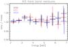 |
Fig. 4 Median and median absolute deviation of the hard band residuals (data/best-fit model) for XIS0 (black), XIS1 (red), and XIS3 (blue). The model is an absorbed single-temperature MEKAL, whose temperatures and metal abundances are independent for each instrument, fitted to 2.0–7.0 keV band using the public calibration. The data are regrouped to a uniform binning of 0.5 keV. |
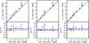 |
Fig. 5 Upper panel: best-fit hard band temperatures (asterisks) and 1σ uncertainties (boxes) for XMM-Newton/EPIC-pn and Suzaku/XIS instruments using the public calibration. The solid black line is an identity line, drawn as a reference. Lower panel: relative temperature differences fT (diamonds) between different XMM-Newton/EPIC-pn and Suzaku/XIS instruments, and their 1σ uncertainties. The dotted and dashed lines show the weighted means of the relative temperature difference and corresponding uncertainties. |
To derive the effects of possible cross-calibration uncertainties in the shape of the effective area in the hard band between Suzaku/XIS and EPIC-pn instruments, we compared the XIS hard band temperatures of our sample to those obtained with EPIC-pn. We found that the XIS1 and EPIC-pn temperatures are consistent within the statistical uncertainties: on average the XIS1 temperatures are ~2% (1.7σ) lower than the EPIC-pn values. XIS0 and XIS3 temperatures are on average ~6% (4.9σ) and ~5% (4.2σ) lower than pn temperatures (see Fig. 5), indicating some cross-calibration problems. However, the lower XIS temperatures may be due to the uncorrected PSF scattering from the cool core, which may bias XIS temperatures low by a maximum of ~6% in the hard band (see Sect. 5.5). Indeed, the stacked XIS/pn residuals indicate some excess data at the lowest energies, reaching a maximum of ~10% at ~3 keV energies, which is possibly due to the PSF scatter from the cool core (see Fig. 6). Since the effective area energy dependence of XMM-Newton’s EPIC-pn is most likely well calibrated in the hard band (Nevalainen et al. 2010), the shape of the hard band effective areas of the XIS instruments are correctly calibrated within the statistical and PSF-related uncertainties, amounting to ~5% uncertainties on the measurement of the hard band temperature.
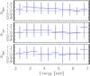 |
Fig. 6 Median ± median absolute deviation of hard energy band stacked residuals of XIS0/pn R0pn (top panel), XIS1/pn R1pn (middle panel) and XIS3/pn R3pn (bottom panel). The data are regrouped to a uniform binning of 0.5 keV. |
7.2. Soft band
The temperature measurement of hot clusters is not optimally achieved in the 0.5–2.0 keV band as the temperature dependence of the continuum shape is relatively weak since the cut-off is at higher energies. Due to weak line emission in the soft energy band at typical cluster temperatures, possible uncertainties in metal abundance measurements mostly produce variation in continuum emission, which in turn may affect the temperature measurements. However, our aim here is to achieve a phenomenological, rather than physical model of the combination of cluster continuum emission and effective area calibration uncertainties. Thus the soft band temperatures are still useful for the purposes of cross-calibration of the effective area.
7.2.1. Temperatures and residuals
We fitted the soft band spectra of the clusters in the soft band sample with an absorbed single-temperature MEKAL model (see Table A.1). The soft band temperatures obtained using XIS1 and XIS3 differ by ~9%, which is not very significant (2.9σ). Unfortunately, XIS0 temperatures disagree significantly compared to the other two instruments. They are on average ~29% (11.2σ) and ~23% (7.4σ) lower than the XIS1 and XIS3 temperatures (see Fig. 7).
Ishida et al. (2011) provided results on PKS2155-304 that also indicate that XIS0 yields softer spectra than XIS1 in the 0.5–2.0 keV band during 2005–2008, which is qualitatively consistent with our cluster results. However, as noted in Sect. 7.1, Ishida et al. (2011) used an older XIS calibration with a different model for the OBF contaminant, making a more rigorous comparison to that work difficult.
XIS soft band residuals exhibit a systematic behaviour: they reach a maximum at 1.3–1.4 keV while they decrease with lower and higher energy (see Fig. 8). We attempted two-temperature modelling, but this did not significantly improve the spectral fits. Importantly, the residuals of the XIS0 unit, which yielded significantly lower soft band temperatures (see above) are rather consistent with unity below 1 keV energies, while those of XIS1 and XIS3 decrease significantly below unity. Assuming for a moment that the shape of the XIS0 effective area below 1 keV is accurately calibrated, this indicates that the effective areas of XIS1 and XIS3 are increasingly overestimated with lower energy.
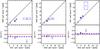 |
Fig. 7 Upper panel: best-fit soft band temperatures (asterisks) and 1σ uncertainties (boxes) for Suzaku/XIS instruments using the public calibration. The solid black line is an identity line, drawn as a reference. Lower panel: relative temperature differences fT (diamonds) between different Suzaku/XIS instruments, and their 1σ uncertainties. The dotted and dashed lines show the weighted means of the relative temperature difference and corresponding uncertainties. |
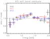 |
Fig. 8 Median and median absolute deviation of the residuals (data/best-fit model) of the soft band cluster sample for XIS0 (black), XIS1 (red), and XIS3 (blue). The model is an absorbed single-temperature MEKAL, whose temperatures and metal abundances are independent for each instrument, fitted to 0.5–2.0 keV band using the public calibration. The data are regrouped to a uniform binning of 127.75 keV. |
The comparison between XIS and XMM-Newton/pn soft band temperatures complicates the situation further: XIS0 values are on average ~14% (6.2σ) lower than those of pn, whereas XIS1 and XIS3 values are on average ~18% (7.4σ) and ~9% (3.0σ) higher than those of pn (see Fig. 9). Because PSF scatter from the cool core could bias XIS temperatures low by 7% in only the worst case, this effect is unable to fully account for the XIS0/pn temperature difference, and in fact any correction for it would exacerbate the XIS1/pn and XIS3/pn differences.
The observations of PKS2155-304 (Ishida et al. 2011) also indicate that XIS1 yields harder spectra than pn in the 0.5–2.0 keV energy band. Because Chandra/ACIS soft band cluster temperatures are on average ~20% higher than pn soft band temperatures (Nevalainen et al. 2010), XIS1/ACIS are the only instrument pair that yields approximately consistent sample average soft band temperatures. Due to these disagreements we have no clear indications of which instruments are most accurately calibrated in the soft energy band.
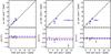 |
Fig. 9 Upper panel: best-fit soft band temperatures (asterisks) and 1σ uncertainties (boxes) for XMM-Newton/EPIC-pn and Suzaku/XIS instruments using the public calibration. The solid black line is an identity line, drawn as a reference. Lower panel: relative temperature differences fT (diamonds) between XMM-Newton/EPIC-pn and Suzaku/XIS instruments, and their 1σ uncertainties. The dotted and dashed lines show the weighted means of the relative temperature difference and corresponding uncertainties. |
7.2.2. Stacked residuals
However, this unfortunate situation does not prohibit us from deriving information about XIS cross-calibration by analysing the cluster measurements. The above XIS temperature and residual discrepancies are indicative of uncertainties of the cross-calibration of the energy dependence of the effective area of different XIS instruments. Because XIS1 as a back-illuminated (BI) device has the largest effective area of the three XIS CCDs, we adopted it as the reference instrument for a relative cross-calibration comparison between the XIS instruments using the stacked residuals method (see Sect. 6.3). The analysis indicated a systematic difference between the cross-calibration of the XIS0/XIS1 effective areas, which increases towards lower energies (see Fig. 10). The median of XIS0/XIS1 residuals reaches a value of ~1.2 at 0.5 keV, indicating ~20% cross-calibration uncertainties. The case of XIS3/XIS1 is less problematic, since the median of XIS3/XIS1 differs significantly from unity only in the energy bin at ~0.5–0.7 keV.
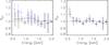 |
Fig. 10 Median ± median absolute deviation of soft energy band stacked residuals of XIS0/XIS1 R01 (left panel) and XIS3/XIS1 R31 (right panel) using the public calibration (dotted line) and the modified responses described in this work (solid line). The data are regrouped to a uniform binning of 127.75 keV. |
To evaluate the cross-calibration uncertainties of the soft band effective area shape between Suzaku/XIS and XMM-Newton/pn instruments, indicated by the differences of the soft band temperatures (see Sect. 7.2.1), we calculated the stacked residuals using EPIC-pn as the reference instrument (Fig. 11). While XIS0/pn residuals are rather consistent with unity at the lowest energies, the data indicate that at energies above 1.3 keV XIS0 flux is lower than EPIC-pn flux by ~10%. This effect would account for the systematically lower soft band XIS0 temperatures compared to EPIC-pn. On the other hand, the XIS1 and XIS3 instruments yield ~10–20% lower flux than EPIC-pn at energies below 1 keV. This results in higher soft band temperatures for XIS1 and XIS3 compared to EPIC-pn.
However, we have no indications of which instrument is the most accurately calibrated in the soft band. We therefore conclude that if fitting only soft band data (0.5–2.0 keV), as is often done for high-redshift clusters whose emission in the hard band is low compared to the background, using Suzaku/XIS or EPIC-pn instruments, the cross-calibration uncertainties between these instruments yield a maximum systematic uncertainty of ~30% on the derived temperatures.
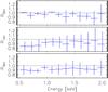 |
Fig. 11 Median ± median absolute deviation of the soft energy band stacked residuals of XIS0/pn R0pn (top panel), XIS1/pn R1pn (middle panel) and XIS3/pn R3pn (bottom panel). The data are regrouped to a uniform binning of 127.75 keV. |
7.3. Full band
We then proceeded to evaluate the effects of the above cross-calibration uncertainties on standard astrophysical spectral analysis of the cluster spectra, i.e. modelling and analysis of the full useful energy band of 0.5–7.0 keV, using the soft band sample. These results should be applicable for any type of source that produces such continuum-dominated X-ray emission in this energy band which has significant statistical weight at energies below 2 keV. However, the using a singe-temperature emission model in the full band may not be physically justified because of a possible multi-temperature structure of the intracluster medium. Indeed, while the XIS residuals show systematic features due to the calibration uncertainties discussed above, a part of the residuals may originate from multi-temperature structures (see Fig. 12). Yet using the single-temperature emission model has the advantage of yielding a simple and useful measure for cross-calibration uncertainties.
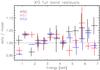 |
Fig. 12 Median and median absolute deviation of the residuals (data/best-fit model) for the soft band cluster sample when fitting the full 0.5–7.0 keV band using the public calibration for XIS0 (black), XIS1 (red), and XIS3 (blue). The model is an absorbed single-temperature MEKAL, whose temperatures and metal abundances are independent for each instrument. The data are regrouped to a uniform binning of 0.5 keV. |
7.3.1. Temperatures
While the cross-calibration uncertainties between XIS instruments and between Suzaku/XIS and EPIC-pn instruments were quite large below 2 keV (see Sect. 7.2), the largest discrepancies were concentrated in a rather narrow energy band of 0.5–0.8 keV (see Figs. 10, 11). The emission of this band is relatively small when compared to the total emission of the full band and thus the effect of the soft band discrepancies on full band temperatures is small. The full band analysis resulted in temperatures quite similar to the well-calibrated hard band8.
Comparison of best-fit temperatures using the full band showed that the effect of the lowest energy XIS cross-calibration uncertainties to the full band temperatures are ~3%. The effect of Suzaku/XIS/EPIC-pn soft energy calibration uncertainties on the full band temperatures is ~1–5%, depending on the XIS instrument (see Fig. 13).
7.3.2. Stacked residuals
When using the stacked residuals method to evaluate the cross-calibration uncertainties of the effective area, a very detailed physically sound model is not necessary: using the stacked residuals formula (Eq. (1)) will take into account and correct for the deviations of the best-fit model and the data of the reference instrument. Assuming that the calibration of the reference instrument is correct, the phenomenological model (i.e. the best-fit model corrected for the deviations with the data) derived for the reference instrument still yields a prediction that matches the data of the instrument, if its calibration is accurate.
Yet the stacked residuals for XIS instruments (using XIS1 as a reference as before) in the full band yield systematic differences at energies above 2 keV (Fig. 14), inconsistent with the above argumentation and the fact that in the hard band we found a very good agreement between the different XIS instruments (Figs. 3 and 4). We think that the reason for this is that the sample used for the hard band studies is larger than the one used for the soft and full band study due to our selection criteria (Sect. 2). In the hard band the dispersion of the residuals of individual clusters is higher for the smaller sample where one or two deviant objects may cause the difference. Thus, the full band stacked residuals analysis above 2 keV energies should be taken with caution.
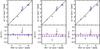 |
Fig. 13 Upper panel: best-fit full band temperatures (asterisks) and 1σ uncertainties (boxes) for XMM-Newton/EPIC-pn and Suzaku/XIS instruments using the public calibration. The solid black line is an identity line, drawn as a reference. Lower panel: relative temperature differences fT (diamonds) between XMM-Newton/EPIC-pn and Suzaku/XIS instruments, and their 1σ uncertainties. The dotted and dashed lines show the weighted means of the relative temperature difference and corresponding uncertainties. |
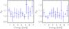 |
Fig. 14 Median ± median absolute deviation of the full energy band stacked residuals of XIS0/XIS1 R01 (left panel) and XIS3/XIS1 R31 (right panel) using the public calibration. Note that the cluster sample used here is different from the one used for the hard band. The data are regrouped to a uniform binning of 0.5 keV. |
A similar problem is present when analysing the stacked residuals of the XIS instruments using EPIC-pn as a reference instrument: while the XIS/pn stacked hard band residuals showed a very good consistence (Figs. 5 and 6), the stacked XIS/pn residuals of the smaller sample used for the full band (Fig. 15) exhibit systematic differences at energies above 2 keV. As above, we think that the differences of the samples are causing this discrepancy, and that the XIS/pn cross-calibration uncertainties above 2 keV are better evaluated using the larger hard band sample. Thus, with the current data we cannot properly estimate the effect of the full band cross-calibration uncertainties between the Suzaku/XIS instruments and between the Suzaku/XIS and the EPIC-pn instruments.
7.4. Suzaku old calibration
To study the effects of the different calibration versions on the discrepancies detected in the XIS data in both hard and soft energy bands, we additionally reprocessed the data with the previous Suzaku ftools version 17. The older version (XIS CALDB release 20110210) differs mainly by containing the previous model for the XIS contamination (ae_xi*_contami_ 20081023.fits for XIS1 and XIS3, and ae_xi*_contami_ 20090128.fits for XIS0) where the carbon-to-oxygen ratio was fixed to 6.0.
The different calibration versions changed the best-fit hard energy band temperatures by less than 0.1% and the soft energy band temperatures by less than 3.5%. Thus, temperature discrepancies and consistencies reported above also apply to the old calibration. We did not study the effects of different XIS calibration versions in any more detail.
8. Fluxes
In addition to the cross-calibration of the shape of the effective area, the cluster data can also be used to assess the cross-calibration of the normalisation of the effective area. To the first order the flux of the cluster emission depends linearly on the accuracy of the normalisation of the effective area. Due to the differences of the composition of the samples used for the analysis of the hard and soft band (see Sect. 2), we only studied fluxes in the hard band here.
We examined the hard band fluxes given by the best-fit unabsorbed MEKAL models presented in (Sect. 7.1). We calculated the fluxes and their statistical uncertainties using the cflux model in Xspec. Due to masked point sources, bad columns, and pn CCD gaps, the covered fraction of the 3–6 arcmin annulus used for spectral extraction varies between the instruments. To enable a meaningful comparison of fluxes we calculated the flux in terms of mean surface brightness by dividing the total flux from the extraction region with the useful detector area for each cluster. Since the emission is not constant with radius, the difference in covered areas might introduce some differences to the flux of a given cluster measured with different instruments.
We found that the hard band fluxes measured with XIS instruments agree within a 2% statistical uncertainty. As indicated by the hard band stacked residuals (Fig. 6), EPIC-pn fluxes are on average lower than those obtained with the XIS0, XIS1, and XIS3 instruments, with the difference amounting to ~10% (32.5σ), ~6% (20.7σ) and ~6% (18.9σ) (see Table 4). For Suzaku/XIS instruments the object-dependent fraction of the PSF scatter of photons from the cluster core to the 3–6 arcmin extraction region might affect the observed fluxes. For clusters A1795 and A3112 with the brightest cool cores in our sample, we estimated in Sect. 5.5 that in maximum ~15% of the photons in the extraction region may be scattered from the cool core. The fraction is expected to be lower for other clusters in our sample. Thus, XIS fluxes might be biased high and a correction for the PSF effect would accordingly yield fluxes more consistent with EPIC-pn.
Since the Chandra/ACIS instrument has been reported to yield ~10% higher fluxes than EPIC-pn in the hard band (Nevalainen et al. 2010), we find perfect agreement between XIS0 and ACIS fluxes and XIS1 and XIS3 are in closer agreement with ACIS than pn. However, correcting XIS fluxes for the maximum PSF scatter of ~15% would move all XIS instruments to a closer agreement with pn than ACIS. Thus the comparison if XIS hard band fluxes are consistent with pn or ACIS is inconclusive. We also note that hard band XIS/pn cross-calibration uncertainties (Fig. 6) yield a maximum systematic uncertainty of ~10% to the derived fluxes.
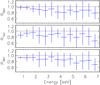 |
Fig. 15 Median ± median absolute deviation full band stacked residuals of XI0/pn (R0pn, top panel), XIS1/pn (R1pn, middle panel) and XIS3/pn (R3pn, bottom panel). The data are regrouped to a uniform binning of 0.5 keV. |
Fluxes in the hard energy band given by the unabsorbed MEKAL model.
9. Suzaku OBF contamination
We examine here whether possible uncertainties in the modelling of the Suzaku OBF contaminant could explain the problems in the cross-calibration of the effective areas of the different XIS instruments we reported above.
It has long been observed that the XIS optical blocking filter (OBF) suffers from contamination on the spacecraft side9. The contaminant is unknown, but is thought to consist of oxygen, hydrogen, and carbon, and possibly arises from a DEHP-like material that has been created by evaporation from the spacecraft components. The instrumental and temporal variability of the contaminant in the public Suzaku calibration (which used contamination file ae_xi*_contami_20091201.fits) is modelled using observations of 1E0102-72.3 and RXJ1856.5-3754. The hydrogen-to-carbon number density ratio is assumed to be a constant 157.61, whereas the oxygen-to-carbon ratio varies with time as10 (2)where MJD is the Mean Julian Day of the observation. The spatial variability of the contaminant is measured with monthly integrated observations of the sun-lit Earth. The contaminant is assumed to have the same composition in all parts of the detector, but its column density varies as a function of radius from the centre of the detector as
  (3)where r is the radius in arcmin, NC (t,r = 0) is the column density of the contaminant at time t in the centre of the detector, and A(t) and B(t) are time dependent constants.
Since the absorption of the contaminant is strongest in the soft energy band (see Fig. 16), possible uncertainties of the column densities of the oxygen and carbon in the current public calibration of the contaminant may contribute to the soft band uncertainties we reported above (Sect. 7.2).
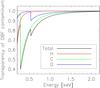 |
Fig. 16 Total (black) transparency of the OBF contaminant as a function of energy with contributions of individual elements O (blue), C (green), and H (red) for a contaminant with NO = 0.80 × 1018 cm-2 and a composition corresponding to an observation date of 2006-10-27 (approximately coincident with the the mean observation date of our soft band sample), i.e. oxygen-to-carbon ratio of 0.20 and hydrogen-to-carbon ratio of 157.61. |
Indeed, if we adopt an estimate for the systematic uncertainty from on-axis calibration measurements11 and vary the amount of the 2006-10-27 contaminant (see Fig. 16) by 1–3σ, i.e. vary the oxygen column density by 0.5–1.5 × 1017 cm-2 while keeping the relative abundance of other elements constant, the effective area changes increasingly with lower energy (see Fig. 17). This yields the same level of difference (~20% at 0.5 keV) as indicated by the Suzaku/XIS0/XIS1 and XIS3/XIS1 cluster observations (see Fig. 10). Because the change of the oxygen column density does not cause any effect in the hard band, agreement of the XIS instruments with EPIC-pn in the hard band is maintained (Sect. 7.1). This makes a possible uncertainty in the oxygen and carbon column densities a feasible cause for the problems in the cross-calibration of XIS soft band effective areas.
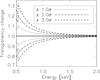 |
Fig. 17 Change of the transparency of the 2006-10-27 OBF contaminant when the oxygen column density is varied by ±1.0σ (dotted lines), 2.0σ (dashed and dotted lines), and 3.0σ (dashed lines) while keeping the relative abundance of the other elements fixed. |
9.1. Spectral analysis of OBF column densities
9.1.1. Method
We proceeded by quantitatively testing the hypothesis that the reported systematic uncertainties of the oxygen column density (Sect. 9) are responsible for the soft band XIS calibration problems (Fig. 10). The test includes modifying the XIS effective areas with a physically motivated absorption model for the contaminant and requiring that all instruments produce an equal emission model for a given cluster.
We adopted the model used by the Suzaku calibration team as the absorption model, with absorption cross-sections from Balucinska-Church & McCammon (1992). We determined the oxygen-to-carbon ratio for each cluster according to the observation date using the time dependence (Eq. (2)) and used the hydrogen-to-carbon ratio of the contaminant in the public calibration12. By allowing the oxygen column density to vary, we thus varied the total amount of the contaminant, while keeping the composition of the model consistent with the contaminant implemented in the public calibration.
We multiplied the MEKAL emission model with the above absorption model, while forcing the temperature and metal abundance to be equal in all instruments for a given cluster. We allowed the normalisation of the emission model for a given cluster to be an independent parameter for the different instruments. We created auxiliary response files assuming no contaminant, and used these to fit the product of the MEKAL model and absorption model. While maintaining the emission models equal between all instruments for a given cluster, the fit to data determines the required oxygen column density, i.e. we fitted the effective areas simultaneously with the cluster emission.
9.1.2. Quality of the modelling
By regrouping the spectra to a uniform binning of 127.75 eV (see Sect. 7.2.1), we found that the above modification to XIS effective areas in all cases improves the fits over fits made with the public calibration (Figs. 8 and 18; Tables 6 and A.1). The improvement is clearly significant, as is evident from visual inspection of the residuals. However, the standard F-test evaluation of the improvement in terms of the decrease of χ2 relative to the decrease of the degrees of freedom is not applicable here. While the χ2 in the modified ARF fits decrease, there are more degrees of freedom in the modified ARF fits than in the public ARF fits, because the number of free parameters in the public ARF fits is 9 (three temperatures, three abundances, and three normalisations) while in the modified ARF fits the number of free parameters is 8 (one temperature, one abundance, three normalisations, and three values of NO)13.
Modified oxygen column density of the OBF contaminant in joint XIS fits.
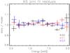 |
Fig. 18 Median and median absolute deviation of the residuals (data/best-fit model) of the soft band cluster sample for XIS0 (black), XIS1 (red), and XIS3 (blue). The model is an absorbed single-temperature MEKAL, whose temperatures and metal abundances are forced to be equal in all instruments for a given cluster, fitted to 0.5–2.0 keV band using the effective areas modified with the contaminant model. |
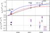 |
Fig. 19 Upper panel: time dependence of the oxygen column densities and 1.0 σ statistical uncertainties of the contaminant fitted to the cluster data (diamonds) and the ones implemented in the public calibration at 4.5 arcmin distance from the centre of the FOV (lines) for XIS0 (black), XIS1 (red), and XIS3 (blue). Lower panel: time dependence of the difference. |
9.1.3. Modification to the contaminant
When we apply the stacked residuals method (Sect. 7.2.2) to the results with the modified effective areas, we find that the median of the ratios R01 and R31 become close to unity (Fig. 10). These estimates of the effective area cross-calibration uncertainties show a clear improvement over those obtained with the public calibration. The stacked residuals with modified ARFs are consistent with unity in all channels except 0.5–0.6 keV for the XIS3/XIS1 ratio. This implies that while the current public H–C–O composition with modified column density yields a significant improvement over the column density implemented in the current public calibration, there may still be room for adjusting the composition of the contaminant and other constituents of the effective area.
To evaluate the cluster-based modification to the column density of the contaminant implemented in the current calibration, we need to work out the values of the oxygen column density in our 3–6 arcmin extraction regions in the public calibration, since these are not available in the auxiliary response files produced by the standard software.
Currently, the radial behaviour of the contaminant (Eq. (3)), which is essential for extended sources like clusters, is only measured for the XIS1 instrument and assumed to be equal for XIS0 and XIS3. This is a possible source of remaining calibration uncertainties that we cannot examine with the current data. We divided our 3–6 arcmin extraction regions into concentric annuli with a width of 0.5 arcmin and calculated the NO of the public calibration at the centres of these annuli. We weighted these values with the flux in each annulus using the surface brightness profiles of Nevalainen et al. (2010) for A1795, A262, and A3112; the profiles of Markevitch et al. (1999) for A496 and those of Tamura et al. (2000) for A1060, to recover the NO values in the current calibration. The flux in the annuli remains rather constant with radius due to the opposing effects of the radially decreasing surface brightness and the radially increasing area of the annuli. The flux-weighted average oxygen column densities are within ±1% of that at a distance of 4.5 arcmin from the centre of the FOV, which we used to evaluate the oxygen column densities of the contaminant for our clusters in the public calibration.
Most of the modified oxygen column densities (see Fig. 19 and Table 5) are within 3σ of the reported uncertainties of the values implemented in the public calibration (see Sect. 9). In more detail, the cluster analysis indicated that the NO values of XIS0 are very close to the public calibration values up to May 2008 while XIS1 and XIS3 require an additional oxygen column density of the contaminant up to 2 × 1017 cm-2. This implies that the soft band effective area shape of XIS0 is currently accurately calibrated and that the effective area of XIS1 and XIS3 is increasingly overestimated towards the lowest energies in the public calibration for observations up to to May 2008.
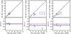 |
Fig. 20 Upper panel: best-fit soft band temperatures (asterisks) and 1σ uncertainties (boxes) for Suzaku/XIS instruments using the modified XIS effective area (joint fit) and public calibration. The solid black line is an identity line, drawn as a reference. Lower panel: relative temperature differences fT (diamonds) between the Suzaku/XIS instruments, and their 1σ uncertainties. The dotted and dashed lines show the weighted means of the relative temperature difference and corresponding uncertainties. |
All instruments require a significant increase of the oxygen column density for the A496 observation in Aug. 2008. This effect is not evident in the monitoring data of E0102-7214. This may be affected by the fact that the Galactic NH varies by ~2 × 1020 cm-2 within 1° from the cluster centre (Kalberla et al. 2005). Also, allowing the column density to be a free parameter, Tanaka et al. (2006) derived an NH profile for A496 that increases towards the cluster centre, reaching a maximum of ~6 × 1020 cm-2 in the 3–6 arcmin annulus, while we used the LAB average of ~4 × 1020 cm-2 in our fits. From consideration of the transmission curves (see Fig. 16), we conclude that this discrepancy in the Galactic NH can account for the extra contaminant required in the fits to A496.
9.1.4. New cluster emission models
Since the required modification of the XIS0 effective area yields only minor changes for the oxygen column density of the contaminant (see Fig. 19), the corresponding changes in the XIS0 temperatures are small (see Fig. 20, and Tables 6 and A.1). The required higher NO for XIS1 and XIS3 increases the absorption and to produce the same model prediction, the emission models become softer. On average the XIS1 and XIS3 temperatures decrease by ~27% (11.5σ) and ~22% (7.4σ), respectively, compared to the fit with the public calibration.
Best-fit parameters of joint XIS spectral fits with modified contaminant.
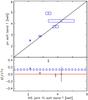 |
Fig. 21 Upper panel: best-fit soft band temperatures (asterisks) and 1σ uncertainties (boxes) for EPIC-pn and Suzaku/XIS instruments using the modified XIS effective area. The solid black line is an identity line, drawn as a reference. Lower panel: relative temperature differences fT (diamonds) between EPIC-pn and Suzaku, and their 1σ uncertainties. The dotted and dashed lines show the weighted means of the relative temperature difference and corresponding uncertainties. |
Since the soft band temperatures of XIS1 and XIS3 decrease significantly with the modification of the contaminant, the Suzaku/XIS v.s. EPIC-pn soft band temperature comparison will change from that using the public calibration, presented in Sect. 7.2.1. The joint XIS0 + XIS1 + XIS3 fit to the soft band with the free contaminant yielded on average ~12% (6.2σ) lower temperatures compared to EPIC-pn soft bands temperatures (see Fig. 21). As noted in Sect. 5.5, the PSF scattering from cool cores may bias XIS best-fit temperatures low by 7% in the worst case; however, we expect this bias to be much smaller in most cases. If corrected for the PSF scatter, the XIS soft band temperatures might increase by a few %, i.e., become closer to the EPIC-pn values. Since the Chandra/ACIS instrument has been found to yield ~18% higher temperatures than EPIC-pn in the soft band (Nevalainen et al. 2010), our results indicate that the XIS instruments yield a better soft band temperature agreement with the EPIC-pn instrument than with the Chandra/ACIS instrument. The data exhibit quite a lot of scatter: three of the clusters yield consistent values between Suzaku/XIS and EPIC-pn, while the temperatures of two of the clusters differ by 4.9σ and 7.1σ.
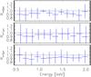 |
Fig. 22 Median ± median absolute deviation of the soft energy band stacked residuals of XIS0/pn Rm0pn (top panel), XIS1/pn Rm1pn (middle panel) and XIS3/pn Rm3pn (bottom panel) using the contamination-modified effective areas for XIS instruments. The data are regrouped to a uniform binning of 127.75 keV. |
With the introduction of the modified contaminate the Suzaku/XIS1,3 and EPIC-pn stacked soft band residuals at the lowest energies become consistent with unity, while XIS0 and pn remain consistent in both cases (compare Figs. 11 and 22). However, the scatter is larger (10–20%) when using the modified contaminate, and thus the remaining energy-dependent uncertainties, which amount to 12% temperature differences (see above), are not significantly detected with the current data.
10. Conclusions
We used a sample of galaxy clusters to perform a study on the accuracy of the cross-calibration of the energy dependence and the normalisation of the effective area of the XIS0, XIS1, and XIS3 instruments onboard Suzaku and the EPIC-pn instrument onboard XMM-Newton in 3–6 arcmin annular extraction regions. The Suzaku results apply to the XIS CALDB versions 20110608 (i.e. public calibration at the time of writing of this paper) and 20110201, and to XRT CALDB version 20080709 for observations carried out during 2005–2008. The XMM-Newton results refer to SAS version xmmsas_20110223_1801-11.0.0 and the latest calibration information in June 2011. The results are summarised in Fig. 23 and Table 7.
Relative difference (μ) and significance (sig.) of the temperatures and fluxes obtained with different instrument combinations.
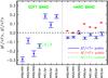 |
Fig. 23 Average relative difference (diamonds) ± the error of the mean of the temperatures (solid line) and fluxes (dotted line) using the public calibration in the soft band (left side of the plot) and in the hard band (right side of the plot). Comparison of the pn and XIS soft band temperature using the modification to the contaminant is shown with diamonds and dashed lines. |
Because the shape of the spectrum determining the temperature of the cluster depends on the energy dependence of the effective area and the flux depends on the normalisation of the effective area, we compared the temperatures, fluxes, and best-fit emission models of the clusters measured with different instruments in the 0.5–2.0 and 2.0–7.0 keV bands.
Comparison of the Suzaku/XIS instruments with each other yielded that XIS0 and XIS3 produced rather consistent hard band temperatures that are systematically lower than those obtained with XIS1 by ~5%. The Suzaku/XIS hard band temperatures are systematically lower than those obtained with the EPIC-pn instrument of XMM-Newton, but only by 2–6% on average. Some fraction of this difference could be caused by Suzaku’s PSF scattering from the cool core, which should be less than ~6% in the worst case. Since EPIC-pn hard band temperatures are consistent with Chandra/ACIS and BeppoSAX/MECS temperatures, and EPIC-pn bremsstrahlung temperatures agree with Fe XXV/XXVI line ratio temperatures (Nevalainen et al. 2010), we suggest that the energy dependence of XIS instruments is quite accurately calibrated in the hard band. The remaining calibration uncertainties may yield effects on the XIS hard band temperatures at an ~6% level.
In the soft 0.5–2.0 keV energy band the XIS1 and XIS3 instruments yielded consistent temperatures when using the public calibration, while XIS0 yielded temperatures that are lower by an average of 29% (11.2σ) and 23% (7.4σ) than those obtained with XIS1 and XIS3, respectively. Comparison of the residuals showed that the XIS0 effective area is underestimated or that the XIS1 and XIS3 effective area is overestimated towards lower energies, with the difference increasing to ~20% at 0.5 keV.
We tested the assumption that these discrepancies in the effective area in the soft band are caused by uncertainties of the implemented column density of the optical blocking filter (OBF) contaminant. We achieved this by allowing the OBF contaminant to have a column density different from that in the public calibration and jointly fitting the XIS0 + XIS1 + XIS3 soft band spectral data, while forcing the temperatures and metal abundances to be equal in all instruments for a given cluster. The resulting fits to the data were significantly better than those using the public calibration. Assuming the composition of the contaminant as in the public calibration, we found that the cluster data required an addition to the column density of the contaminant of XIS1 and XIS3 amounting to a maximum ΔNO of 2 × 1017 cm-2, i.e. at a 4σ level of the reported uncertainties of the NO measurements in the public calibration. The column density of the XIS0 contaminant implemented in the public calibration is consistent with that obtained in our spectral analysis of clusters. Thus, the analysis implies that the effective area of XIS0 in the soft band is more accurately modelled in the public calibration than that of XIS1 and XIS3 for observations during 2005–2008.
The XIS soft band temperatures obtained with the modified effective area are lower by ~12% than those obtained with EPIC-pn instrument onboard XMM-Newton. Considering that the PSF scatter from the cool cores may bias the XIS soft band temperatures low, the PSF-corrected XIS soft band temperatures would agree better with those obtained using EPIC-pn. However, the Chandra/ACIS instrument yields ~18% higher temperatures than EPIC-pn in the soft band (Nevalainen et al. 2010). Thus, our results indicate that the XIS instruments yield a better soft band temperature agreement with the EPIC-pn instrument than with the Chandra/ACIS instrument.
The hard band fluxes derived with Suzaku/XIS instruments are higher than those derived with EPIC-pn by ~6–10%, whereas the Chandra/ACIS instrument yields ~10% higher fluxes than EPIC-pn in the hard band (Nevalainen et al. 2010). However, because the Suzaku/XIS fluxes might be biased high by a maximum of ~15% due to PSF scatter and the Suzaku/XIS and EPIC-pn hard band data show that the derived fluxes have a maximum systematic uncertainty of ~10%, the comparison of Suzaku/XIS to EPIC-pn and Chandra/ACIS fluxes proved inconclusive.
See e.g. http://heasarc.gsfc.nasa.gov/Tools/xraybg_help.html for references.
The differences in the hard and wide band samples also play a role here, see Sect. 7.3.2.
See e.g. http://space.mit.edu/XIS/monitor/
from http://space.mit.edu/XIS/monitor/contam/. Because we use off-axis extraction regions, uncertainties in the spatial dependence of the contaminant will somewhat increase the actual systematic uncertainty for our extraction region. The systematic uncertainties of the calibration measurements dominate over the statistical uncertainties.
Because the spectral fit parameters relating to the sky background (see Sect. 5.1) are forced to be equal in all instruments for modified ARF fits, the difference in degrees of freedom increases even more.
Acknowledgments
We would like to acknowledge IACHEC members and thank L. David, K. Hamaguchi, H. Matsumoto, M. Nobukawa and M. Stühlinger for useful comments. K.K. acknowledges support from Magnus Ehrnrooth foundation and Nylands Nation. E.D.M. acknowledges support from NASA grant NNX09AE58G to MIT. This research has made use of data obtained from the High Energy Astrophysics Science Archive Research Center (HEASARC), provided by NASA’s Goddard Space Flight Center.
References
- Balucinska-Church, M., & McCammon, D. 1992, ApJ, 400, 699 [NASA ADS] [CrossRef] [Google Scholar]
- Cash, W. 1979, ApJ, 228, 939 [NASA ADS] [CrossRef] [Google Scholar]
- Fujimoto, R., Mitsuda, K., Mccammon, D., et al. 2007, PASJ, 59, 133 [NASA ADS] [Google Scholar]
- Grevesse, N., & Sauval, A. J. 1998, SSRv, 85, 161 [Google Scholar]
- Ishida, M., Tsujimoto, M., Kohmura, T., et al. 2011, PASJ, 63, 657 [Google Scholar]
- Kalberla, P. M. W., Burton, W. B., Hartmann, D., et al. 2005, A&A, 440, 775 [NASA ADS] [CrossRef] [EDP Sciences] [Google Scholar]
- Koyama, K., Tsunemi, H., Dotani, T., et al. 2007, PASJ, 59, 23 [Google Scholar]
- Lehto, T., Nevalainen, J., Bonamente, M., Ota, N., & Kaastra, J. 2010, A&A, 524, A70 [NASA ADS] [CrossRef] [EDP Sciences] [Google Scholar]
- Longinotti, A. L., de La Calle, I., Bianchi, S., Guainazzi, M., & Dovciak, M. 2008, Rev. Mex. Astron. Astrofis. Conf. Ser., 32, 62 [NASA ADS] [Google Scholar]
- Markevitch, M., Vikhlinin, A., Forman, W. R., & Sarazin, C. L. 1999, ApJ, 527, 545 [NASA ADS] [CrossRef] [Google Scholar]
- Mewe, R., Kaastra, J., & Liedahl, D. 1995, Legacy, 6, 16 [Google Scholar]
- Nevalainen, J., Markevitch, M., & Lumb, D. 2005, ApJ, 629, 172 [NASA ADS] [CrossRef] [Google Scholar]
- Nevalainen, J., David, L., & Guainazzi, M. 2010, A&A, 523, A22 [NASA ADS] [CrossRef] [EDP Sciences] [Google Scholar]
- Peres, C. B., Fabian, A. C., Edge, A. C., et al. 1998, MNRAS, 298, 416 [NASA ADS] [CrossRef] [Google Scholar]
- Reiprich, T. H., & Böhringer, H. 2002, ApJ, 567, 716 [NASA ADS] [CrossRef] [Google Scholar]
- Sato, K., Yamasaki, N. Y., Ishida, M., et al. 2007, PASJ, 59, 299 [NASA ADS] [Google Scholar]
- Snowden, S. L., Collier, M. R., & Kuntz, K. D. 2004, ApJ, 610, 1182 [NASA ADS] [CrossRef] [Google Scholar]
- Strüder, L., Briel, U., Dennerl, K., et al. 2001, A&A, 365, L18 [NASA ADS] [CrossRef] [EDP Sciences] [Google Scholar]
- Tamura, T., Makishima, K., Fukazawa, Y., Ikebe, Y., & Xu, H. 2000, ApJ, 535, 602 [NASA ADS] [CrossRef] [Google Scholar]
- Tanaka, T., Kunieda, H., Hudaverdi, M., Furuzawa, A., & Tawara, Y. 2006, PASJ, 58, 703 [NASA ADS] [CrossRef] [Google Scholar]
- Vikhlinin, A., Markevitch, M., Murray, S. S., et al. 2005, ApJ, 628, 655 [NASA ADS] [CrossRef] [Google Scholar]
- Wargelin, B. J., Markevitch, M., Juda, M., et al. 2004, ApJ, 607, 596 [Google Scholar]
Appendix A: Spectral fits
Here we show the data and the best-fit single temperature MEKAL models for EPIC-pn (Fig. A.1), XIS0 (Fig. A.2), XIS1 (Fig. A.3) and XIS3 (Fig. A.4) using the public calibration. The spectral parameters are listed in Table A.1.
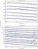 |
Fig. A.1 Soft band (upper panel) and hard band (lower panel) XMM-Newton/EPIC-pn spectra (crosses) and best-fit single temperature independent fits (solid lines) for the cluster sample. The normalisations of the spectra are adjusted for plot clarity and do not reflect the relative brightness of the clusters. |
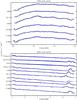 |
Fig. A.2 Soft band (upper panel) and hard band (lower panel) Suzaku/XIS0 spectra (crosses) and best-fit single temperature independent fits (solid lines) for the cluster sample. The normalisations of the spectra are adjusted for plot clarity and do not reflect the relative brightness of the clusters. |
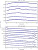 |
Fig. A.3 Soft band (upper panel) and hard band (lower panel) Suzaku/XIS1 spectra (crosses) and best-fit single temperature independent fits (solid lines) for the cluster sample. The normalisations of the spectra are adjusted for plot clarity and do not reflect the relative brightness of the clusters. |
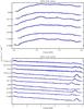 |
Fig. A.4 Soft band (upper panel) and hard band (lower panel) Suzaku/XIS3 spectra (crosses) and best-fit single temperature independent fits (solid lines) for the cluster sample. The normalisations of the spectra are adjusted for plot clarity and do not reflect the relative brightness of the clusters. |
Best-fit parameters of the Suzaku/XIS and XMM-Newton/EPIC-pn spectral fits using the public calibration.
All Tables
Relative difference (μ) and significance (sig.) of the temperatures and fluxes obtained with different instrument combinations.
Best-fit parameters of the Suzaku/XIS and XMM-Newton/EPIC-pn spectral fits using the public calibration.
All Figures
|
Fig. 1 XIS1 raw count rate maps (not corrected for background or vignetting) of the soft band cluster sample in a 0.5–7.0 keV energy band binned to 8 pixels (~0.14 arcmin) per bin. The inner and outer radii of the 3–6 arcmin extraction region are denoted by white circles, the green circles show the excluded regions centred on point sources seen in XMM-Newton/EPIC-pn images. Scaling of the maps is adjusted for clarity and does not reflect the relative brightness of the clusters. The colour bar shows the the total number of counts per bin. |
| In the text | |
|
Fig. 2 Total emission (blue crosses), sky background (black curve), and non X-ray background (red crosses) emission of A496 in the 3–6 arcmin region for XIS1. The sky background is modelled from ROSAT All Sky Survey data and folded through the XIS1 response. The XIS1 observation of A496 has the strongest relative background emission of the cluster sample. |
| In the text | |
|
Fig. 3 Upper panel: best-fit hard band temperatures (asterisks) and 1σ uncertainties (boxes) for Suzaku/XIS instruments using the public calibration. The solid black line is an identity line, drawn as a reference. Lower panel: relative temperature differences fT (diamonds) between different Suzaku/XIS instruments, and their 1σ uncertainties. The dotted and dashed lines show the weighted means of the relative temperature difference and corresponding uncertainties. |
| In the text | |
|
Fig. 4 Median and median absolute deviation of the hard band residuals (data/best-fit model) for XIS0 (black), XIS1 (red), and XIS3 (blue). The model is an absorbed single-temperature MEKAL, whose temperatures and metal abundances are independent for each instrument, fitted to 2.0–7.0 keV band using the public calibration. The data are regrouped to a uniform binning of 0.5 keV. |
| In the text | |
|
Fig. 5 Upper panel: best-fit hard band temperatures (asterisks) and 1σ uncertainties (boxes) for XMM-Newton/EPIC-pn and Suzaku/XIS instruments using the public calibration. The solid black line is an identity line, drawn as a reference. Lower panel: relative temperature differences fT (diamonds) between different XMM-Newton/EPIC-pn and Suzaku/XIS instruments, and their 1σ uncertainties. The dotted and dashed lines show the weighted means of the relative temperature difference and corresponding uncertainties. |
| In the text | |
|
Fig. 6 Median ± median absolute deviation of hard energy band stacked residuals of XIS0/pn R0pn (top panel), XIS1/pn R1pn (middle panel) and XIS3/pn R3pn (bottom panel). The data are regrouped to a uniform binning of 0.5 keV. |
| In the text | |
|
Fig. 7 Upper panel: best-fit soft band temperatures (asterisks) and 1σ uncertainties (boxes) for Suzaku/XIS instruments using the public calibration. The solid black line is an identity line, drawn as a reference. Lower panel: relative temperature differences fT (diamonds) between different Suzaku/XIS instruments, and their 1σ uncertainties. The dotted and dashed lines show the weighted means of the relative temperature difference and corresponding uncertainties. |
| In the text | |
|
Fig. 8 Median and median absolute deviation of the residuals (data/best-fit model) of the soft band cluster sample for XIS0 (black), XIS1 (red), and XIS3 (blue). The model is an absorbed single-temperature MEKAL, whose temperatures and metal abundances are independent for each instrument, fitted to 0.5–2.0 keV band using the public calibration. The data are regrouped to a uniform binning of 127.75 keV. |
| In the text | |
|
Fig. 9 Upper panel: best-fit soft band temperatures (asterisks) and 1σ uncertainties (boxes) for XMM-Newton/EPIC-pn and Suzaku/XIS instruments using the public calibration. The solid black line is an identity line, drawn as a reference. Lower panel: relative temperature differences fT (diamonds) between XMM-Newton/EPIC-pn and Suzaku/XIS instruments, and their 1σ uncertainties. The dotted and dashed lines show the weighted means of the relative temperature difference and corresponding uncertainties. |
| In the text | |
|
Fig. 10 Median ± median absolute deviation of soft energy band stacked residuals of XIS0/XIS1 R01 (left panel) and XIS3/XIS1 R31 (right panel) using the public calibration (dotted line) and the modified responses described in this work (solid line). The data are regrouped to a uniform binning of 127.75 keV. |
| In the text | |
|
Fig. 11 Median ± median absolute deviation of the soft energy band stacked residuals of XIS0/pn R0pn (top panel), XIS1/pn R1pn (middle panel) and XIS3/pn R3pn (bottom panel). The data are regrouped to a uniform binning of 127.75 keV. |
| In the text | |
|
Fig. 12 Median and median absolute deviation of the residuals (data/best-fit model) for the soft band cluster sample when fitting the full 0.5–7.0 keV band using the public calibration for XIS0 (black), XIS1 (red), and XIS3 (blue). The model is an absorbed single-temperature MEKAL, whose temperatures and metal abundances are independent for each instrument. The data are regrouped to a uniform binning of 0.5 keV. |
| In the text | |
|
Fig. 13 Upper panel: best-fit full band temperatures (asterisks) and 1σ uncertainties (boxes) for XMM-Newton/EPIC-pn and Suzaku/XIS instruments using the public calibration. The solid black line is an identity line, drawn as a reference. Lower panel: relative temperature differences fT (diamonds) between XMM-Newton/EPIC-pn and Suzaku/XIS instruments, and their 1σ uncertainties. The dotted and dashed lines show the weighted means of the relative temperature difference and corresponding uncertainties. |
| In the text | |
|
Fig. 14 Median ± median absolute deviation of the full energy band stacked residuals of XIS0/XIS1 R01 (left panel) and XIS3/XIS1 R31 (right panel) using the public calibration. Note that the cluster sample used here is different from the one used for the hard band. The data are regrouped to a uniform binning of 0.5 keV. |
| In the text | |
|
Fig. 15 Median ± median absolute deviation full band stacked residuals of XI0/pn (R0pn, top panel), XIS1/pn (R1pn, middle panel) and XIS3/pn (R3pn, bottom panel). The data are regrouped to a uniform binning of 0.5 keV. |
| In the text | |
|
Fig. 16 Total (black) transparency of the OBF contaminant as a function of energy with contributions of individual elements O (blue), C (green), and H (red) for a contaminant with NO = 0.80 × 1018 cm-2 and a composition corresponding to an observation date of 2006-10-27 (approximately coincident with the the mean observation date of our soft band sample), i.e. oxygen-to-carbon ratio of 0.20 and hydrogen-to-carbon ratio of 157.61. |
| In the text | |
|
Fig. 17 Change of the transparency of the 2006-10-27 OBF contaminant when the oxygen column density is varied by ±1.0σ (dotted lines), 2.0σ (dashed and dotted lines), and 3.0σ (dashed lines) while keeping the relative abundance of the other elements fixed. |
| In the text | |
|
Fig. 18 Median and median absolute deviation of the residuals (data/best-fit model) of the soft band cluster sample for XIS0 (black), XIS1 (red), and XIS3 (blue). The model is an absorbed single-temperature MEKAL, whose temperatures and metal abundances are forced to be equal in all instruments for a given cluster, fitted to 0.5–2.0 keV band using the effective areas modified with the contaminant model. |
| In the text | |
|
Fig. 19 Upper panel: time dependence of the oxygen column densities and 1.0 σ statistical uncertainties of the contaminant fitted to the cluster data (diamonds) and the ones implemented in the public calibration at 4.5 arcmin distance from the centre of the FOV (lines) for XIS0 (black), XIS1 (red), and XIS3 (blue). Lower panel: time dependence of the difference. |
| In the text | |
|
Fig. 20 Upper panel: best-fit soft band temperatures (asterisks) and 1σ uncertainties (boxes) for Suzaku/XIS instruments using the modified XIS effective area (joint fit) and public calibration. The solid black line is an identity line, drawn as a reference. Lower panel: relative temperature differences fT (diamonds) between the Suzaku/XIS instruments, and their 1σ uncertainties. The dotted and dashed lines show the weighted means of the relative temperature difference and corresponding uncertainties. |
| In the text | |
|
Fig. 21 Upper panel: best-fit soft band temperatures (asterisks) and 1σ uncertainties (boxes) for EPIC-pn and Suzaku/XIS instruments using the modified XIS effective area. The solid black line is an identity line, drawn as a reference. Lower panel: relative temperature differences fT (diamonds) between EPIC-pn and Suzaku, and their 1σ uncertainties. The dotted and dashed lines show the weighted means of the relative temperature difference and corresponding uncertainties. |
| In the text | |
|
Fig. 22 Median ± median absolute deviation of the soft energy band stacked residuals of XIS0/pn Rm0pn (top panel), XIS1/pn Rm1pn (middle panel) and XIS3/pn Rm3pn (bottom panel) using the contamination-modified effective areas for XIS instruments. The data are regrouped to a uniform binning of 127.75 keV. |
| In the text | |
|
Fig. 23 Average relative difference (diamonds) ± the error of the mean of the temperatures (solid line) and fluxes (dotted line) using the public calibration in the soft band (left side of the plot) and in the hard band (right side of the plot). Comparison of the pn and XIS soft band temperature using the modification to the contaminant is shown with diamonds and dashed lines. |
| In the text | |
|
Fig. A.1 Soft band (upper panel) and hard band (lower panel) XMM-Newton/EPIC-pn spectra (crosses) and best-fit single temperature independent fits (solid lines) for the cluster sample. The normalisations of the spectra are adjusted for plot clarity and do not reflect the relative brightness of the clusters. |
| In the text | |
|
Fig. A.2 Soft band (upper panel) and hard band (lower panel) Suzaku/XIS0 spectra (crosses) and best-fit single temperature independent fits (solid lines) for the cluster sample. The normalisations of the spectra are adjusted for plot clarity and do not reflect the relative brightness of the clusters. |
| In the text | |
|
Fig. A.3 Soft band (upper panel) and hard band (lower panel) Suzaku/XIS1 spectra (crosses) and best-fit single temperature independent fits (solid lines) for the cluster sample. The normalisations of the spectra are adjusted for plot clarity and do not reflect the relative brightness of the clusters. |
| In the text | |
|
Fig. A.4 Soft band (upper panel) and hard band (lower panel) Suzaku/XIS3 spectra (crosses) and best-fit single temperature independent fits (solid lines) for the cluster sample. The normalisations of the spectra are adjusted for plot clarity and do not reflect the relative brightness of the clusters. |
| In the text | |
Current usage metrics show cumulative count of Article Views (full-text article views including HTML views, PDF and ePub downloads, according to the available data) and Abstracts Views on Vision4Press platform.
Data correspond to usage on the plateform after 2015. The current usage metrics is available 48-96 hours after online publication and is updated daily on week days.
Initial download of the metrics may take a while.