| Issue |
A&A
Volume 551, March 2013
|
|
|---|---|---|
| Article Number | A20 | |
| Number of page(s) | 7 | |
| Section | Cosmology (including clusters of galaxies) | |
| DOI | https://doi.org/10.1051/0004-6361/201220282 | |
| Published online | 12 February 2013 | |
Diffuse light in the young cluster of galaxies CL J1449+0856 at z = 2.07⋆
1 LAM, OAMP, Université Aix-Marseille CNRS, Pôle de l’Étoile, Site de Château Gombert, 38 rue Frédéric Joliot-Curie, 13388 Marseille 13 Cedex, France
e-mail: This email address is being protected from spambots. You need JavaScript enabled to view it.
2 UPMC-CNRS, UMR 7095, Institut d’Astrophysique de Paris, 98bis Bd Arago, 75014 Paris, France
3 Núcleo de Astrofísica Teórica, Universidade Cruzeiro do Sul, R. Galvão Bueno 868, 01506–000 São Paulo, Brazil
Received: 24 August 2012
Accepted: 23 December 2012
Abstract
Context. Cluster properties do not seem to be changing significantly during their mature evolution phase; for example, they do not seem to show any strong dynamical evolution at least up to z ~ 0.5, their galaxy red sequence is already in place at least up to z ~ 1.2, and their diffuse light content remains stable up to z ~ 0.8. The question is now to know if cluster properties can evolve more significantly at redshifts that are notably higher than 1.
Aims. We propose here to see how the properties of the intracluster light (ICL) evolve with redshift by detecting and analysing the ICL in the X-ray cluster CL J1449+0856 at z = 2.07, based on deep HST NICMOS H band exposures.
Methods. We used the same wavelet-based method as one applied to 10 clusters between z = 0.4 and 0.8.
Results. We detect three diffuse light sources with total magnitudes of H = 24.8, 25.5, and 25.9, plus a more compact object with a magnitude H = 25.3. We discuss the significance of our detections and show that they are robust.
Conclusions. The three sources of diffuse light indicate an elongation along a north-east south-west axis, similar to that of the distribution of the central galaxies and to the X-ray elongation. This strongly suggests a history of merging events in this direction. While we found a roughly constant amount of diffuse light for clusters between z ~ 0 and 0.8, we prove at least a 1.5 mag increase between z ~ 0.8 and 2. If we assume that the amount of diffuse light is directly linked to the infall activity on the cluster, this implies that CL J1449+0856 is still undergoing strong merging events.
Key words: galaxies: clusters: individual: CL J1449+0856
The data presented in this paper were obtained from the Mikulski Archive for Space Telescopes (MAST). STScI is operated by the Association of Universities for Research in Astronomy, Inc., under NASA contract NAS5-26555. Support for MAST for non-HST data is provided by the NASA Office of Space Science via grant NNX09AF08G and by other grants and contracts. This research has made use of data from HST-COSMOS project, held in the HST-COSMOS database operated by Cesam, Laboratory of Astrophysics of Marseille.
© ESO, 2013
1. Introduction
Clusters of galaxies are the final product of a long-term hierarchical accretion process, starting with the first matter density concentrations visible in the cosmic microwave background and continuing until the present day with still growing massive clusters such as Coma. We can define at least three benchmarks in the cluster-building process.
First, the presently favoured cosmological Lambda cold dark matter (ΛCDM) model predicts that the first massive structures should appear around z ~ 2. More quantitatively, Romer et al. (2001), for example, have shown that structures hotter than 2 keV should not be found in a ΛCDM universe with Ωm = 0.3 approximately beyond this redshift. Temperatures of 2 keV can be considered as the lowest possible values for clusters, group temperatures being closer to 1 keV (e.g. Fig. 7 of Ulmer et al. 2005). That the highest redshift confirmed massive structures are located around z ~ 2.1 (Gobat et al. 2011) is in good agreement with this model (as long as other massive structures are not detected at significantly higher redshifts).
After having reached this initial (somewhat arbitrary) temperature of 2 keV, clusters continue to grow accreting matter from their surrounding filaments. This growth is probably mainly driven by accretion of already formed groups (e.g. Adami et al. 2005a). At redshifts close to two, such events could be considered as major mergers between more or less equally massive structures, because the impactor (the infalling group) is not significantly less massive than the impacted structure (the “cluster”). At lower redshifts, the impacted structure has gained mass, while infalling groups are still of low mass, so we reach a situation where fusions are becoming minor. This allows us to define a second crucial step in the cluster history, which corresponds to the epoch (around z ~ 1, see Appendix A) where infalling groups are becoming significantly less massive than the accreting cluster.
Clusters then mainly grow through minor fusions until they (hypothetically) reach a virialized state. However, such virialized clusters are very rare, even if a few are known at z ~ 0 (e.g. A496, Durret et al. 2000). This shows that clusters have generally not yet reached this third step. We have therefore defined two main epochs in the cluster history: their initial accretion phase between z ~ 2 and 1, and their mature growth at redshifts lower than 1.
There is accumulating evidence that cluster properties do not change very significantly during their mature evolution phase. Even if their galaxy populations show variations during this period, with more lenticular and fewer late type galaxies at z ~ 0 than at z ~ 1, clusters do not seem, for example, to show strong dynamical evolution at least up to z ~ 0.5 (e.g. Adami et al. 2000), their galaxy red sequence is already in place at least up to z ~ 1.2 (e.g. Bremer et al. 2006), and their diffuse light content remains stable up to z ~ 0.8 (Guennou et al. 2012).
The question is now to know if cluster properties evolve more significantly at redshifts notably higher than one. This is a new field of investigation since very few clusters are known in this redshift interval. We propose in this paper to pave the way for the cluster’s diffuse light content by trying to detect this cluster baryonic component at z ~ 2.1 in the structure discovered by Gobat et al. (2011).
Diffuse light becomes an important aspect in clusters of galaxies as shown by recent studies (Gregg & West 1998; Mihos et al. 2005; Zibetti et al. 2005; González et al. 2007; Krick & Bernstein 2007; Rudick et al. 2010; Burke et al. 2012). It finds its origin at least partly in matter ejections from galaxies during galaxy-galaxy or galaxy-cluster potential interactions (see e.g. Adami et al. 2005b; or Dolag et al. 2010, for recent simulations). More intense interactions should therefore lead to a larger amount of diffuse light in clusters, and by detecting diffuse light we can evaluate the infalling activity on a cluster.
Galaxy evolution and “pre-processing” in groups, prior to their infall in clusters, also play important roles in the content of diffuse light in mature clusters (Fujita 2004; Rudick et al. 2006). The amount of pre-processing will depend on the characteristics of the infalling group, such as density and dynamical evolution stage (Da Rocha & Mendes de Oliveira 2005; Da Rocha et al. 2005, 2008).
Guennou et al. (2012) used deep HST ACS data to detect diffuse light for ten clusters between z = 0.4 and 0.8 and did not detect any significant variation in the cluster diffuse light content with redshift. By applying a somewhat less sophisticated method, Burke et al. (2012) extended this search to a sample of six clusters at z ~ 1 based on VLT/HAWK-I data, and found that intracluster light (hereafter ICL) only composed (1−4)% of the total cluster light.
Playing the same game at higher redshift is a difficult task, since extremely deep images are required to beat the cosmological dimming factor acting on extended sources following a (1 + z)4 law. The need for images with very low sky background is even more crucial at redshifts significantly higher than 1, given the surface brightness of the searched sources. This clearly speaks in favour of space-based images. Finally, such a search requires redder bands as we go to higher redshifts, because the diffuse light usually detected in clusters is rather red, and therefore probably not forming stars (e.g. Adami et al. 2005b). We therefore need to use photometric bands sensitive to old stellar populations at the considered redshift (typically redder than the rest-frame V band). At z ≥ 1, this eliminates all visible bands, leaving us only with NIR bands.
Combining these three requirements drastically reduces the number of clusters with suitable data available. The Gobat et al. (2011) z = 2.07 structure is one of them. As one of the very rare z ≥ 1.5 clusters with a measured X-ray temperature hotter than 2 keV, it has been observed with the NICMOS HST near infrared camera in the F160W band (close to the H band) with a ~20 ks exposure time. Such data should make it possible to detect diffuse light sources only about five times brighter in flux than the typical Coma sources, by applying the same wavelet technique as in Guennou et al. (2012).
Section 2 describes the data. Section 3 describes the method and presents our detections. Section 4 deals with the detection robustness. Section 5 deals with the source redshift, and Sect. 6 is the discussion. We adopted the concordance cosmological model (ΩLambda = 0.74, Ωm = 0.26). All magnitudes are given in the AB system.
2. Data
As previously stated, we downloaded the HST NICMOS H band data for the CL J1449+0856 cluster (observing program 11174, PI: E. Daddi). The data consist of two separate exposures of 7680 and 10 240 s in the F160W filter. This cluster, with a centre at α = 222.3092°,δ = +8.9404° (see Gobat et al. 2011) also shows extended X-ray emission, and is at a redshift of 2.07. Gobat et al. (2011) estimated its mass to (5.3−8) × 1013 M⊙.
The F160W filter at z = 2.07 is more or less equivalent to the F814W filter for clusters at z ~ 0.56. This is close to the mean redshift of the cluster sample analysed by Guennou et al. (2012) based on data taken with the F814W filter and analysed with the same method we apply here. We are therefore in a very favourable situation to compare the results of the present study with those of Guennou et al. (2012).
We used the NICMOS-pipelined mosaic images. This reduction is suitable for our purposes because it only removes a constant sky level, and therefore does not remove potential large-scale diffuse light sources. We then extracted a 134 × 162 pixel2 area centred on the cluster position. This eliminated portions of the initial images strongly affected by flat field residuals (see also Sect. 4).
We finally combined the two images to create a ~18 ks F160W image. This was made with the Scamp and Swarp softwares (Bertin et al. 2002; Bertin 2006) without background removal in order not to erase diffuse light sources because of the Spline background estimate method used by Swarp.
We note that the cluster does not occupy the same place on the NICMOS detector in the two individual images, minimizing the effect of flat field and detector artefacts in our analysis.
3. Method and results
3.1. The use of the OV_WAV package
We applied the same wavelet-based method (the OV_WAV package, see e.g. Pereira 2003; Da Rocha & Mendes de Oliveira 2005) to detect diffuse light as applied to ten clusters between z = 0.4 and 0.8 by Guennou et al. (2012). A similar method was also used for the Coma cluster (z = 0.023, Adami et al. 2005b) and Abell 2667 (z = 0.233, Covone et al. 2006). We are therefore in the position of discussing the full cluster history, from z ~ 0 to z ~ 2.1. We briefly summarize below the method that we applied. We only give the salient points of the technique in this section and refer the reader to Pereira (2003) and Da Rocha & Mendes de Oliveira (2005) for more details.
OV_WAV is a multi-scale vision model (e.g. Rué & Bijaoui 1997). After applying a wavelet transform to an observation of the targeted cluster, we identified the statistically significant pixels in the wavelet transform space (at the 5σ level). To define the objects, the selected pixels were then grouped in connected fields for each given scale. An inter-scale connectivity tree is then established, and we identified each connected tree containing connected fields of significant pixels across three or more scales. We can then associate them with the objects. An individual image is finally recovered for each identified object, with an iterative reconstruction algorithm.
In a first step, we detected small-scale objects in the sky image to produce our object image. We considered characteristic scales between 1 and 32 pixels in wavelet space, adapted to the size of the NICMOS images. The object image was then subtracted from the sky image to produce the residual image (Fig. 1 left). This residual image includes both hidden features that are typically too faint to satisfy the wavelet first-pass thresholding conditions (fixed at 5σ) and the diffuse light sources. We finally detect objects in this residual image on characteristic scales between 1 and 16 pixels, to create a second object image.
In a second step we searched for what we call the real ICL sources, i.e. extended low surface-brightness features in the residual image. These features were detected in this image by considering the pixels where the signal is larger than 2.5σ compared to an empty area of the residual image (Fig. 1 shows the 2.5 and 3σ levels as red contours). Each of these sources was visually inspected before the removal of obvious numerical residuals of bright saturated Galactic stars or defects due to image cosmetics. This was done by subtracting a Sinc function (see Appendix B) with the orientation of the SExtractor detected objects. The amplitude of the Sinc function was scaled to the SExtractor object magnitudes. We note that the three diffuse light sources that we discuss in the following were detected as objects by OV_WAV in the second object image, melted with numerical residuals. This is why we used the residual image to locate these diffuse light sources.
3.2. Detected sources
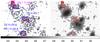 |
Fig. 1 Right: F160W HST NICMOS image (100 kpc wide) of CL J1449+0856. Left: residual image. Blue ellipses are SExtractor detected objects at a threshold of 1.4. Red contours are computed from the residual image. Contours start at the 2.5σ level and have a 0.5σ increment. We also give the H-band surface brightness scale and the integrated magnitudes of the detected sources. |
We display our results in Fig. 1. Objects that are wavelet-detected in the first pass are compact and also nearly all SExtractor-detected. The residual image (Fig. 1 left) includes three diffuse light sources (S1, S2, S3) and probably a compact low signal-to-noise object (indicated as Obj 1). We also show the blue rectangles in which we measured the magnitudes for S1, S2, S3, and Obj 1. S1, S2, and S3 have respective total magnitudes of H = 24.8 ± 0.13, 25.5 ± 0.21, and 25.9 ± 0.34 (see next section). Their mean surface brightness are 25.95, 26.0, and 26.3. This amount of diffuse light in CL J1449+0856 roughly corresponds to an L∗ field galaxy at z ~ 2 (e.g. Ilbert et al. 2005). This is a similar amount to what we found in the Coma cluster (Adami et al. 2005b). Obj 1 is a compact object with a total magnitude of H = 25.3.
We note that the S1 source is located 2.4 arcsec from the optical centre of CL J1449+0856. At z = 2.07, this translates to almost 20 kpc, typical of the clustercentric distances found for the diffuse light sources of Guennou et al. (2012). This also means that such a study is impossible with classical ground-based data where the typical seeing is of the order of 1 arcsec.
4. Detection robustness
4.1. Simulations
We first address the question of the theoretical detection limit of our method with the data in hand. Considering the simulations by Guennou et al. (2012), OV_WAV should not allow us to detect Coma-like 2.5σ diffuse light sources at z greater than 0.8 in 10 ks F814W HST ACS exposures. Assuming a (1 + z)4 dimming factor, the same rest-frame wavelength, and an exposure of 18 ks, this implies that we could only detect sources 1.7 mag/arcsec2 brighter than Coma-like sources at z = 2.07 with F160W at the 2.5σ level, and sources 1.2 mag/arcsec2 brighter than Coma-like sources at z = 2.07 with F160W at the 2σ level. However, these estimates are based on two different instruments (ACS versus NICMOS) and related to different redshifts and observed wavelength ranges (already formed clusters at z ≤ 1 versus a young cluster just at the beginning of its formation at z ~ 2).
We therefore redid simulations similar to those of Guennou et al. (2012). We simulated sources of uniform surface brightnesses with ten pixel diameters, which we scaled to different surface brightnesses before inserting them into the NICMOS images of CL J1449+0856. This size is typical of the sources we detect in CL J1449+0856. As in Guennou et al. (2012), we performed this exercice ten times for each simulated surface brightness. This allowed us to quantify our ability to detect sources of diffuse light, as well as the purity of our detections (how many fake sources we are detecting).
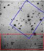 |
Fig. 2 H-band NICMOS image of CL J1449+0856. The blue rectangle is the region centred on the cluster itself, and the red rectangle is the region with the strongest flat-field residuals. |
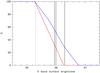 |
Fig. 3 Percentage of recovered diffuse light sources as defined in the text versus H-band surface brightness. Blue line: percentage in the cluster region. Red line: percentage in the high noise region (see Fig. 2). The three vertical solid lines show the surface brightness of the three real diffuse light sources. The vertical dotted line is the surface brightness of Obj1 as shown in Fig. 1. |
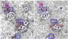 |
Fig. 4 Residual images computed on the individual exposures (left: 7680 s, right: 10 240 s). The red contours show the 2σ detection level. The blue ellipses are the SExtractor-detected objects. The blue rectangles show the locations of the diffuse light sources detected in the summed image (see Fig. 1). |
Knowing that relatively strong flat field residuals are affecting the external parts of the HST NICMOS images, we can ask what this effect contributes to the diffuse light detection. We therefore performed the described simulations in two areas. The first one is centred on the cluster, and the second one is located in the image region that is the most affected by flat field residuals (see Fig. 2).
We show the results in Fig. 3. We see that we are able to detect 100% of the diffuse light sources down to a brightness of H ~ 25.2 mag arcsec-2. The detection percentage then decreases rapidly when considering the image region that is strongly affected by flat field residuals to reach a zero efficiency for brightness of H ~ 26.2 mag arcsec-2. On the other hand, we see that we can detect sources down to H ~ 26.8 mag arcsec-2 in the cluster region. These results are in good agreement with our detections. Obj1 (see Fig. 1) is located just at the limit of the full detection range, while the three diffuse light sources are located in the decreasing part of the blue curve in Fig. 3. We note that the faintest diffuse light source would not have been detected if it had been located in the high flat field residual region. Figure 3 also implies that we possibly miss diffuse light sources with brightnesses fainter than H ~ 26.8 mag arcsec-2 in our detections, so our estimate of the total amount of diffuse light in CL J1449+0856 is only a lower limit.
Finally Fig. 3 shows that our results are probably only weakly affected by fake detections because no such detections occur for very faint brightnesses (where we theoretically are unable to detect our simulated sources). This means that our purity is higher than 90%: less than one fake detection is occuring among our ten simulations.
With these simulations, we were also able to estimate the typical uncertainty on the magnitudes of S1, S2, and S3, computed as the 1σ variation of the recovered surface brightnesses. This allowed us to estimate the magnitude uncertainties given in Sect. 3.2.
4.2. Individual exposures
Another test is to try to detect diffuse light sources in each of the two individual NICMOS images in order to estimate the robustness of our detections. Since the cluster does not fall at the same place on the detector in the two exposures, flat field problems should not affect the detection of diffuse light in the same way. We do not expect to detect S1, S2, and S3 at better than the 2σ level in individual exposures, but that they could be visible in each of the two individual images would give confidence in our summed-image detections. We show in Fig. 4 the residual images obtained for the two individual exposures. The 2σ level detections are similar to the results obtained with the 18 ks combination. S1 is not significantly detected in the 7680 s exposure, but appears in the 10 240 s exposure. S2 also seems to appear in both exposures, while S3 and Obj1 are detected in the two individual images. Detection levels are low (2σ versus 2.5σ for the combined image), as expected, but this gives confidence in our detections performed on the 18 ks combined image.
5. Redshift of the diffuse light sources
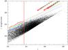 |
Fig. 5 Mean F814W surface brightness (see text) versus I-band (F814W) total magnitude. Black dots: Cosmos (Scoville et al. 2007) HST ACS detected objects with a 68% photometric redshift error lower than 0.2 and a photometric redshift between 0.1 and 6. Only one object over 100 is shown for clarity. Red circles (Elliptical1 in the Cosmos templates), blue dots (Sa0 in the Cosmos templates), and green crosses (Sd0 in the Cosmos templates): the three detected diffuse light sources in CL J1449+0856 assuming different redshifts and different types for the three sources. This allowed us to translate H-band to I-band magnitudes. The vertical red line is the assumed Cosmos completeness total magnitude in terms of surface brightness (I = 23.75: see text). The inclined straight lines show the fits of the Cosmos detection limits (broken lines) computed for total magnitudes I ≤ 23.75 (red: 3σ, green: 2.5σ, blue: 2σ): see also text. |
The next crucial step is to estimate the redshift of the detected diffuse light sources. It is obviously impossible with the instrumentation presently available to measure a spectroscopic redshift for these sources. It is also impossible to compute a photometric redshift with the single available photometric band. We therefore rely on statistical arguments to show that the three detected diffuse light sources are probably members of the CL J1449+0856 cluster. Several objects could mimic cluster diffuse light sources, in particular: (1) relatively bright and single extended objects on the line of sight; and (2) associations of very faint objects.
5.1. Single galaxies along the line of sight?
To test hyphothesis (1), we considered the Cosmos HST-ACS catalogue (Scoville et al. 2007). We computed the mean surface brightness using the Cosmos aperture magnitude measured inside a 0.3 arcsec radius area.
-
This catalogue extends over ~2 deg2, provides objects down to I ~ 26.5 (total magnitude), and theoretically includes all objects (including the faintest possible surface brightness objects) down to I ~ 23.75 (see Fig. 5). The star-galaxy separation is efficient down to I ~ 24. Objects fainter than this limit become so small that even the Cosmos high-resolution images start to be unable to resolve them. Besides the consequences on our surface brightness computation, this also underlines our inability to select pure galaxy samples at these magnitudes.
-
The Cosmos survey does not include H-band measurements, so we had to compute F814W – F160W colours for different redshifts and different spectral types to be able to put our three diffuse light sources on the same plot. This was done with the LePhare tool (Ilbert et al. 2006) between redshifts of 0.1 and 6 and for three different spectral types (Elliptical, Sa, and Sd0 in Fig. 5).
-
We assumed the Cosmos galaxy catalogue complete in terms of surface brightness and not polluted by stars down to I ~ 23.75 (total magnitude). In other words, we assumed that all objects brighter than I ~ 23.75 are detected in the Cosmos survey regardless of their surface brightness and that we can separate stars from galaxies. We then computed the 3σ, 2.5σ, and 2σ Cosmos detection limits in terms of surface brightness down to I ~ 23.75. In other words, for a given total I-band magnitude, we computed the maximal mean surface brightness allowing the detection of 99.7% of the galaxies (i.e. the 3σ level in Fig. 5), of 98.75% of the galaxies (i.e. the 2.5σ level in Fig. 5), and of 95.45% of the galaxies (i.e. the 2σ level in Fig. 5). Finally, we fit straight lines on these broken lines to roughly estimate the surface brightness limitations at fainter total I-band magnitudes to detect galaxies at the 3σ, 2.5σ, and 2σ levels, where objects are too small to be resolved in the considered images. These lines are in fact upper limits, since one would expect that as magnitudes become fainter, the surface brightness limit cannot continue to increase linearly.
Figure 5 shows that less than 0.3% of the Cosmos galaxies could be faint enough in terms of surface brightness to mimic our three diffuse light sources. Considering the density of known Cosmos galaxies on the sky and the spatial extension of our diffuse light sources, we conclude that we only have a 15% chance of having a Cosmos-like galaxy on the line of sight explaining S1, 8% for S2, and 7% for S3. The probability for all three diffuse light sources being explained by Cosmos-like galaxies on the line of sight is therefore lower than 0.1%.
The last possibility in the hypothesis (1) framework would be to have detected large and extremely low surface brightness galaxies on the line of sight, faint enough in surface brightness not to be detected by the Cosmos survey. To test this, we used the field low surface brightness galaxy catalogue detected in Adami et al. (2006). In a 30 × 30 arcmin2 empty sky region, we detected 29 galaxies with B ≤ 25.5 and B surface brightness ≤ 27.2 mag arcsec-2. Assuming a B − I colour varying between one and six (from LePhare computations) between z = 0 and 4, the probability of having such a low surface brightness galaxy in a 10 × 10 arcsec2 area (the presently considered region of interest including S1, S2, and S3) varies between 0.2% and 8%. The probability of having three such galaxies is therefore lower than 0.05%.
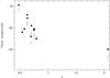 |
Fig. 6 Total absolute magnitude of the detected diffuse light (F814W for the 10 Guennou et al. (2012) clusters to the left, and F160W for CL J1449+0856 to the right). The F160W filter at z = 2.07 is equivalent to the F814W filter for clusters at z ~ 0.56. Filled circles: raw values, crosses: mass normalized values with Fig. 10 of Guennou et al. (2012). Error bars are only plotted for the mass normalized values. The Guennou et al. (2012) points were assumed to be plagued by a ± 0.2 mag error, as suggested by Fig. 10 of this paper. |
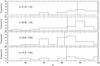 |
Fig. A.1 Histograms of the mass ratios of the most massive infalling structure to the main structure in the Millennium simulation given as percentages, in four redshift bins. The vertical lines show the mean values for each redshift bin. A percentage of 100 means that the most massive infalling structure has the same mass as the main structure. |
5.2. Associations of very faint objects along the line of sight?
Associations of very faint objects along the line of sight (hypothesis 2) could also explain our diffuse light sources. They could be compact classical objects that are spatially correlated. To test this, we considered the Hubble Ultra Deep Field (Beckwith et al. 2006), providing an object catalogue down to i ≤ 29.75 (on a more reduced area than the Cosmos region). Given the spatial density of HUDF objects, only 0.3, 0.17, and 0.15 objects could statistically be located in the S1, S2, and S3 areas. This is clearly not enough to explain an association of objects mimicking our diffuse light sources. The only way to reach such a result would be to have exceptionally detected three extremely distant groups of galaxies in a ~10 × 10 arcsec2 area. Even with the most favourable cluster-cluster angular correlation functions (e.g. Durret et al. 2011), the probability of finding three groups hotter than 2 keV (Romer et al. 2001) in a 10 × 10 arcsec2 area to explain S1, S2, and S3 is completely negligible ( ≤ 10-14).
We can therefore conclude quite securely that the best possibility to have detected three such low surface-brightness objects in such a small area is to have detected diffuse light sources related to the CL J1449+0856 cluster.
6. Discussion
As already stated in this work, the general process of the cluster building history starts by the growth of an initial mass fluctuation. This seed is then fed by infalling matter along the cosmological filaments, mainly in the form of already formed groups of galaxies (in which galaxies are pre-processed). This induces interactions between galaxies, and between infalling galaxies and the cluster potential. The intensity and frequency of these interactions depend on many parameters, such as the stage of dynamical evolution of the infalling groups and of the growing cluster. Interactions induce matter ejections from galaxies through, for example, dynamical friction or tidal disruptions. The signatures of such processes are then directly detectable through intracluster’s diffuse light source detections. Their distribution in a given cluster (assuming that the survival time of these sources is not too long) is therefore expected to give direct indications on the zones where galaxy interactions have taken place and on the directions from which infall has occurred onto the cluster.
We applied this technique to the CL J1449+0856 cluster, comparing the indications given by intracluster diffuse light sources to other indicators: the position of the central galaxies of CL J1449+0856 clearly indicates a north-east/south-west axis. The same orientation is visible in the S1, S2, S3 distribution. This elongation is similar to what is found in X-rays from XMM-Newton data by Gobat et al. (2011, see the white ellipse in their Fig. 1, left) and therefore suggests a history of merging events along this direction.
Similarly, the amount of diffuse light detected in a cluster will also give insight into the intensity of the infall process undergone by the cluster. We show in Fig. 6 the total absolute magnitude (in F814W rest frame for the Guennou et al. sample) of the diffuse light detected in CL J1449+0856 and in the Guennou et al. (2012) clusters as a function of redshift. We give the raw values as well as the mass normalized values, as in Guennou et al. (2012, Fig. 10). We note that these mass normalized values are computed using the relation between mass and amount of diffuse light given in Fig. 10 of Guennou et al. (2012) to take into account the natural tendency of a massive cluster to exhibit larger amount of diffuse light compared to a lower mass cluster. While Guennou et al. (2012) found a more or less constant amount of diffuse light for clusters between z ~ 0 and 0.8, we prove a brightening by at least 1.5 mag between z ~ 0.8 and 2. If we assume that the amount of diffuse light is directly linked to the infall activity on a given cluster, as discussed in Guennou et al. (2012), we have a clear sign here of the intense merging processes going on in CL J1449+0856, as expected for such a young and distant cluster.
Acknowledgments
The authors thank the referee for useful and constructive comments and Johan Richard for his help. We acknowledge long term financial support from the CNES.
References
- Adami, C., Holden, B. P., Castander, F. J., et al. 2000, A&A, 362, 825 [NASA ADS] [Google Scholar]
- Adami, C., Biviano, A., Durret, F., & Mazure, A. 2005a, A&A, 443, 17 [NASA ADS] [CrossRef] [EDP Sciences] [Google Scholar]
- Adami, C., Slezak, E., Durret, F., et al. 2005b, A&A, 429, 39 [NASA ADS] [CrossRef] [EDP Sciences] [Google Scholar]
- Adami, C., Scheidegger, R., Ulmer, M., et al. 2006, A&A, 459, 679 [NASA ADS] [CrossRef] [EDP Sciences] [Google Scholar]
- Beckwith, S. V. W., Stiavelli, M., Koekemoer, A. M., et al. 2006, AJ, 132, 1729 [NASA ADS] [CrossRef] [Google Scholar]
- Bertin, E. 2006, ASPC, 351, 112 [Google Scholar]
- Bertin, E., Mellier, Y., Radovich, M., et al. 2002, ASPC, 281, 228 [Google Scholar]
- Bremer, M. N., Valtchanov, I., Willis, J., et al. 2006, MNRAS, 371, 1427 [NASA ADS] [CrossRef] [Google Scholar]
- Burke, C., Collins, C. A., Stott, J. P., & Hilton, M. 2012, MNRAS, 425, 2058 [Google Scholar]
- Covone, G., Adami, C., Durret, F., et al. 2006, A&A, 460, 381 [NASA ADS] [CrossRef] [EDP Sciences] [Google Scholar]
- Da Rocha, C., & Mendes de Oliveira, C. 2005, MNRAS, 364, 1069 [NASA ADS] [CrossRef] [Google Scholar]
- Da Rocha, C., Ziegler, B. L., & Mendes de Oliveira, C. 2008, MNRAS, 388, 1433 [Google Scholar]
- Dolag, K., Murante, G., & Borgani, S. 2010, MNRAS, 405, 1544 [NASA ADS] [Google Scholar]
- Dunkley, J., Komatsu, E., Nolta, M. R., et al. 2009, ApJS, 180, 306 [NASA ADS] [CrossRef] [Google Scholar]
- Durret, F., Adami, C., Gerbal, D., & Pislar, V. 2000, A&A, 356, 815 [NASA ADS] [Google Scholar]
- Durret, F., Adami, C., Cappi, A., et al. 2011, A&A, 535, A65 [NASA ADS] [CrossRef] [EDP Sciences] [Google Scholar]
- Fujita, Y. 2004, PASJ, 56, 29 [NASA ADS] [Google Scholar]
- Gobat, R., Daddi, E., Onodera, M., et al. 2011, A&A, 526, A133 [NASA ADS] [CrossRef] [EDP Sciences] [Google Scholar]
- Gonzalez, A. H., Zaritsky, D., & Zabludoff, A. I. 2007, ApJ, 666, 147 [NASA ADS] [CrossRef] [Google Scholar]
- Gregg, M. D., West, M. J. 1998, Nature, 396, 549 [NASA ADS] [CrossRef] [Google Scholar]
- Guennou, L., Adami, C., Da Rocha, C., et al. 2012, A&A, 537, A64 [NASA ADS] [CrossRef] [EDP Sciences] [Google Scholar]
- Ilbert, O., Tresse, L., Zucca, E., et al. 2005, A&A, 439, 863 [NASA ADS] [CrossRef] [EDP Sciences] [Google Scholar]
- Ilbert, O., Arnouts, S., McCracken, H. J., et al. 2006, A&A, 457, 841 [NASA ADS] [CrossRef] [EDP Sciences] [Google Scholar]
- Krick, J. E., Bernstein, R. A. 2007, AJ, 134, 466 [Google Scholar]
- Mihos, J. C., Harding, P., Feldmeier, J., & Morrison, H. 2005, ApJ, 631, L41 [NASA ADS] [CrossRef] [Google Scholar]
- Pereira, D. N. E. 2003, Undergraduate Thesis, Univ. Federal do Rio de Janeiro, Brazil [Google Scholar]
- Romer, A. K., Viana, P. T. P., Liddle, A. R., & Mann, R. G. 2001, ApJ, 547, 594 [NASA ADS] [CrossRef] [Google Scholar]
- Rudick, C. S., Mihos, J. C., & McBride, C. 2006, ApJ, 648, 936 [NASA ADS] [CrossRef] [Google Scholar]
- Rudick, C. S., Mihos, J. C., Harding, P., et al. 2010, ApJ, 720, 569 [NASA ADS] [CrossRef] [Google Scholar]
- Rué, F., & Bijaoui, A. 1997, Exp. Astron., 7, 129 [Google Scholar]
- Scoville, N., Aussel, H., Brusa, M., et al. 2007, ApJSS, 172, 1 [NASA ADS] [CrossRef] [Google Scholar]
- Springel, V., White, S. D. M., Jenkins, A., et al. 2005, Nature, 435, 629 [NASA ADS] [CrossRef] [PubMed] [Google Scholar]
- Ulmer, M. P., Adami, C., Covone, G., et al. 2005, ApJ, 624, 124 [NASA ADS] [CrossRef] [Google Scholar]
- Ulmer, M. P., Adami, C., Neto, G. B., et al. 2009, A&A, 503, 399 [NASA ADS] [CrossRef] [EDP Sciences] [Google Scholar]
- Zibetti, S., White, S. D. M., Schneider, D. P., & Brinkmann, J. 2005, MNRAS, 358, 949 [Google Scholar]
Appendix A: Infalling activity on clusters in the Millennium simulation
The approximate redshift where infalling groups are becoming less massive than the accreting cluster can be evaluated using the Millennium simulation (Springel et al. 2005), based on a ΛCDM universe with Ωm = 0.3 and ΩΛ = 0.7 (close to the concordance model of Dunkley et al. 2009). For haloes more massive than 4 × 10¹³ M⊙, we computed in four redshift intervals the ratio (expressed in percentages) between the haloes mass and the maximum mass of the other haloes in a 2.5 Mpc radius (a typical virial radius for clusters) and within 0.01 in redshift. Such neighbors are assumed here to be structures that will be accreted in the future. We show in Fig. A.1 that a cut seems to appear at z ≥ 1 where infalling haloes are closer to the value of the main system mass. The position of this cut is also in good agreement with the expectations of Ulmer et al. (2009), based on the typical relaxation time of a galaxy falling onto a typical cluster. This will obviously have to be confirmed on larger numerical simulations in the future given the relatively small number of massive structures present in the Millenium simulations.
Appendix B: SinC subtraction in the residual image
To remove the numerical artefacts in the residual image better, we subtracted from this image a SinC function centred on each object and scaled to the object magnitude. To test the validity of this approach, we show in Fig. B.1 (black curve) the numerical artefacts coming from the brightest star in the CL J1449+0856 field of view (α = 14:49:14.820; δ = + 08:56:12.70) after the removal of the object image from the sky image (see Sect. 3). These artefacts can be modelled by a SinC function (red curve). The subtraction of this analytical curve will therefore remove the negative and positive annuli circling the central peak, at the cost of oversubtracting this residual central peak.
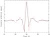 |
Fig. B.1 Black curve: numerical artefacts along the image x-axis coming from the brightest star in the CL J1449+0856 field of view (α = 14:49:14.820; δ = + 08:56:12.70) after removing the object image from the sky image (see Sect. 3). Red curve: SinC modelization. |
All Figures
|
Fig. 1 Right: F160W HST NICMOS image (100 kpc wide) of CL J1449+0856. Left: residual image. Blue ellipses are SExtractor detected objects at a threshold of 1.4. Red contours are computed from the residual image. Contours start at the 2.5σ level and have a 0.5σ increment. We also give the H-band surface brightness scale and the integrated magnitudes of the detected sources. |
| In the text | |
|
Fig. 2 H-band NICMOS image of CL J1449+0856. The blue rectangle is the region centred on the cluster itself, and the red rectangle is the region with the strongest flat-field residuals. |
| In the text | |
|
Fig. 3 Percentage of recovered diffuse light sources as defined in the text versus H-band surface brightness. Blue line: percentage in the cluster region. Red line: percentage in the high noise region (see Fig. 2). The three vertical solid lines show the surface brightness of the three real diffuse light sources. The vertical dotted line is the surface brightness of Obj1 as shown in Fig. 1. |
| In the text | |
|
Fig. 4 Residual images computed on the individual exposures (left: 7680 s, right: 10 240 s). The red contours show the 2σ detection level. The blue ellipses are the SExtractor-detected objects. The blue rectangles show the locations of the diffuse light sources detected in the summed image (see Fig. 1). |
| In the text | |
|
Fig. 5 Mean F814W surface brightness (see text) versus I-band (F814W) total magnitude. Black dots: Cosmos (Scoville et al. 2007) HST ACS detected objects with a 68% photometric redshift error lower than 0.2 and a photometric redshift between 0.1 and 6. Only one object over 100 is shown for clarity. Red circles (Elliptical1 in the Cosmos templates), blue dots (Sa0 in the Cosmos templates), and green crosses (Sd0 in the Cosmos templates): the three detected diffuse light sources in CL J1449+0856 assuming different redshifts and different types for the three sources. This allowed us to translate H-band to I-band magnitudes. The vertical red line is the assumed Cosmos completeness total magnitude in terms of surface brightness (I = 23.75: see text). The inclined straight lines show the fits of the Cosmos detection limits (broken lines) computed for total magnitudes I ≤ 23.75 (red: 3σ, green: 2.5σ, blue: 2σ): see also text. |
| In the text | |
|
Fig. 6 Total absolute magnitude of the detected diffuse light (F814W for the 10 Guennou et al. (2012) clusters to the left, and F160W for CL J1449+0856 to the right). The F160W filter at z = 2.07 is equivalent to the F814W filter for clusters at z ~ 0.56. Filled circles: raw values, crosses: mass normalized values with Fig. 10 of Guennou et al. (2012). Error bars are only plotted for the mass normalized values. The Guennou et al. (2012) points were assumed to be plagued by a ± 0.2 mag error, as suggested by Fig. 10 of this paper. |
| In the text | |
|
Fig. A.1 Histograms of the mass ratios of the most massive infalling structure to the main structure in the Millennium simulation given as percentages, in four redshift bins. The vertical lines show the mean values for each redshift bin. A percentage of 100 means that the most massive infalling structure has the same mass as the main structure. |
| In the text | |
|
Fig. B.1 Black curve: numerical artefacts along the image x-axis coming from the brightest star in the CL J1449+0856 field of view (α = 14:49:14.820; δ = + 08:56:12.70) after removing the object image from the sky image (see Sect. 3). Red curve: SinC modelization. |
| In the text | |
Current usage metrics show cumulative count of Article Views (full-text article views including HTML views, PDF and ePub downloads, according to the available data) and Abstracts Views on Vision4Press platform.
Data correspond to usage on the plateform after 2015. The current usage metrics is available 48-96 hours after online publication and is updated daily on week days.
Initial download of the metrics may take a while.