| Issue |
A&A
Volume 549, January 2013
|
|
|---|---|---|
| Article Number | A73 | |
| Number of page(s) | 17 | |
| Section | Extragalactic astronomy | |
| DOI | https://doi.org/10.1051/0004-6361/201219956 | |
| Published online | 21 December 2012 | |
Multiwavelength campaign on Mrk 509
XII. Broad band spectral analysis
1 UJF-Grenoble 1/CNRS-INSU, Institut de Planétologie et d’Astrophysique de Grenoble (IPAG) UMR 5274, 38041 Grenoble, France
e-mail: pierre-olivier.petrucci@obs.ujf-grenoble.fr
2 ISDC Data Centre for Astrophysics, Astronomical Observatory of the University of Geneva, 16 Ch. d’Ecogia, 1290 Versoix, Switzerland
3 Université de Toulouse, UPS-OMP, IRAP, Toulouse, France
4 CNRS, IRAP, 9 Av. colonel Roche, BP 44346, 31028 Toulouse Cedex 4, France
5 SRON Netherlands Institute for Space Research, Sorbonnelaan 2, 3584 CA Utrecht, The Netherlands
6 Sterrenkundig Instituut, Universiteit Utrecht, PO Box 80000, 3508 TA Utrecht, The Netherlands
7 INAF – IASF Bologna, via Gobetti 101, 40129 Bologna, Italy
8 School of Physics and Astronomy, University of Southampton, Highfield, Southampton SO17 1BJ, UK
9 Centro de Astrobiología (CSIC-INTA), Dep. de Astrofísica; LAEFF, PO Box 78, 28691 Villanueva de la Cañada, Madrid, Spain
10 Space Telescope Science Institute, 3700 San Martin Drive, Baltimore, MD 21218, USA
11 Department of Physics and Astronomy, The John Hopkins University, Baltimore, MD 21218, USA
12 Instituto de Astronomía, Universidad Católica del Norte, Avenida Angamos 0610, Casilla 1280, Antofagasta, Chile
13 Department of Physics, University of Oxford, Keble Road, Oxford OX1 3RH, UK
14 Dipartimento di Fisica, Università degli Studi Roma Tre, via della Vasca Navale 84, 00146 Roma, Italy
15 Mullard Space Science Laboratory, University College London, Holmbury St. Mary, Dorking, Surrey, RH5 6NT, UK
16 Centrum Astronomiczne im. M. Kopernika, Rabiańska 8, 87-100 Toruń, Poland
Received: 6 July 2012
Accepted: 23 September 2012
The origin of the different spectral components present in the high-energy (UV to X-rays/gamma-rays) spectra of Seyfert galaxies is still being debated a lot. One of the major limitations, in this respect, is the lack of really simultaneous broad-band observations that allow us to disentangle the behavior of each component and to better constrain their interconnections. The simultaneous UV to X-rays/gamma rays data obtained during the multiwavelength campaign on the bright Seyfert 1 Mrk 509 are used in this paper and tested against physically motivated broad band models.
Mrk 509 was observed by XMM-Newton and INTEGRAL in October/November 2009, with one observation every four days for a total of ten observations. Each observation has been fitted with a realistic thermal Comptonization model for the continuum emission. Prompted by the correlation between the UV and soft X-ray flux, we used a thermal Comptonization component for the soft X-ray excess. We also included a warm absorber and a reflection component, as required by the precise studies previously done by our consortium. The UV to X-ray/gamma-ray emission of Mrk 509 can be well fitted by these components. The presence of a relatively hard high-energy spectrum points to the existence of a hot (kT ~ 100 keV), optically-thin (τ ~ 0.5) corona producing the primary continuum. In contrast, the soft X-ray component requires a warm (kT ~ 1 keV), optically-thick (τ ~ 10−20) plasma.
Estimates of the amplification ratio for this warm plasma support a configuration relatively close to the “theoretical” configuration of a slab corona above a passive disk. An interesting consequence is the weak luminosity-dependence of its emission, which is a possible explanation of the roughly constant spectral shape of the soft X-ray excess seen in AGNs. The temperature (~3 eV) and flux of the soft-photon field entering and cooling the warm plasma suggests that it covers the accretion disk down to a transition radius Rin of 10 − 20 Rg. This plasma could be the warm upper layer of the accretion disk.
In contrast, the hot corona has a more photon-starved geometry. The high temperature (~100 eV) of the soft-photon field entering and cooling it favors a localization of the hot corona in the inner flow. This soft-photon field could be part of the comptonized emission produced by the warm plasma. In this framework, the change in the geometry (i.e. Rin) could explain most of the observed flux and spectral variability.
Key words: galaxies: active / galaxies: individual: Mrk 509 / galaxies: Seyfert / X-rays: galaxies
© ESO, 2012
1. Introduction
Since the discovery of a high-energy cut-off in the X-ray emission of Seyfert galaxies, first detected by SIGMA and OSSE in NGC 4151 (Jourdain et al. 1992; Maisack et al. 1993) and then commonly observed in about 50% of Seyfert galaxies (Zdziarski et al. 1993; Gondek et al. 1996; Matt 2001; Perola et al. 2002; Deluit & Courvoisier 2003; Dadina 2007; Molina et al. 2009), the primary continuum of this class of AGN is commonly believed to be thermal Comptonization of soft seed photons produced by a “cold phase”, presumably the accretion disk, on hot (~100 keV) thermal electrons (the “hot phase” also called corona). The different Compton scattering orders produced through this process eventually add together to produce a roughly cut-off power-law shape (e.g. Sunyaev & Titarchuk 1980), which agrees well with the high-energy (>2 keV) spectra of Seyfert galaxies.
The nature and origin of this thermal hot plasma are, however, still largely unknown, mainly owing to the lack of sensitive instruments at high energies. This hinders our ability to put tight constraints on the spectral shape and to disentangle the primary continuum from the reflection component. At lower energies (<2 keV), the presence of deep absorption features, the signatures of ionized plasma (the so-called warm absorber, WA hereafter) surrounding the central engine, and soft X-ray emission in excess of the extrapolation of the high-energy continuum to these energies (the so-called soft X-ray excess) does not allow a direct view of the primary emission. Thus, we are generally left with the 2−10 keV band, which is far too narrow for a deep understanding of the origin of the high-energy broad-band emission.
The spectral and flux variability, close to the time scale of a day for black-hole mass of 108 M⊙ but covering a wide frequency range, makes things even more confused if we are not able to separate the contribution of the different spectral components. For example, the X-ray spectral shape of the continuum is expected to harden (the photon index Γ decreases) when the corona temperature (hence the high-energy cut-off) increases (e.g. Haardt et al. 1997). Such variations in the X-ray spectral shape may be produced by intrinsic changes in the corona properties (for example, changes in the heating process efficiency) and/or by variation in the environment like changes of the soft-photon flux (and consequently of the corona cooling) produced by, e.g., the accretion disk.
The origin of the soft X-ray excess has been strongly debated. It was rapidly proposed that it could result from warm Comptonization in an optically thick plasma (e.g. Walter & Fink 1993; Magdziarz et al. 1998, and see more recently Done et al. 2012). In this case, a correlation between the UV and soft X-ray emission is expected. If it is produced by blurred ionized reflection, as proposed by, e.g., Crummy et al. (2006), then the soft X-rays should be linked with the hard (>10 keV) X-rays and reflection components; i.e., a broad iron line and a bump at ~30 keV, are expected. Other authors have explained the soft X-ray excess by smeared absorption (e.g. Gierlinski & Done 2006), but the observations apparently require blurring effects that are too large to be realistic (Schurch et al. 2009). Finally, the effect of partial covering ionized absorption can also account for part of the observed soft excess without requiring material to be moving at extreme velocities (e.g. Miller et al. 2008 and the review of Turner & Miller 2009).
In summary, it is obvious that improving our understanding of Seyfert galaxy high-energy emission requires long and broad-band monitoring.
Mrk 509 is a Seyfert 1 galaxy that harbors a super massive black hole of 1.4 × 10⁸ solar masses (Peterson et al. 2004). It was the object of an intense optical/UV/X-rays/gamma-rays campaign in late 2009, with the participation of five satellites (XMM-Newton, INTEGRAL, Swift, Chandra, and HST) and ground-based telescopes (WHT and PAIRITEL). The source characteristics and the whole campaign are explained in Kaastra et al. (2011). The main objective of this campaign was to study in detail the physical properties and structure of the warm-absorber outflows in Mrk 509. The heart of the monitoring are ten simultaneous XMM-Newton/INTEGRAL observations, with one observation every four days (60 ks with XMM-Newton and 120 ks with INTEGRAL). This paper is part of a series focusing on different results obtained with the campaign. For example, the study of the stacked 600 ks RGS spectrum enabled us to put strong constraints on the outflow nature and geometry (Detmers et al. 2011; Kriss et al. 2011; Kaastra et al. 2012).
Closely related to the present paper, Mehdipour et al. (2011, hereafter M11) have studied the evolution of the UV/X-ray broad-band emission of Mrk 509 using the OM and pn instruments. M11 show that the UV and soft X-ray continuum emission are tightly correlated, suggesting a common origin for the two continuum emission components. This favors an origin through Comptonization instead of blurred absorption or emission, as discussed above. This interpretation has recently been suggested for several narrow-line Seyfert galaxies (Dewangan et al. 2007; Middleton et al. 2009; Jin et al. 2009). The UV/soft X-ray correlation observed in Mrk 509 agrees with the soft X-ray emission being the upper-energy part of the Comptonization of the UV photons in a warm (kT ~ 1 keV) and optically thick (τ ~ 10−20) corona. It is worth noting that these results do not rule out the presence of other components in the soft X-rays (such as blurred reflection or absorptions). But they do not dominate the variability on a time scale of the few days observed during this monitoring.
The study done by M11 was limited to data below 10 keV, and the primary continuum was supposed to be a simple power law. It is known, however, that real Comptonization spectral shapes may be significantly different from a power law (e.g. Haardt 1993; Svensson 1996; Petrucci et al. 2000). Moreover, the interpretation of the spectral variability in terms of physical quantities, such as the temperature and optical depth of the corona, is not straightforward from the photon index and high energy cut-off of a phenomenological cut-off power-law approximation, so it requires the use of approximate formulae to estimate these parameters.
In the present paper we aim at testing realistic Comptonization models in a similar way to the Petrucci et al. (2004) analysis of the simultaneous IUE/RXTE campaign of NGC 7469. The main advantages of the Mrk 509 campaign are that the data cover the X-ray range from the soft X-ray bands up to 200 keV, while the RXTE energy range, in the case of NGC 7469, was limited to 3 − 20 keV. Furthermore, the XMM-Newton data allow us to put strong constraints on the optical/UV continuum and the iron line complex and to analyze the WA structure precisely. Thus, for the first time, we are able to do a broad-band spectral analysis of UV to X-ray data of a Seyfert galaxy, on a month’s time scale, including all the major spectral components known to be present in this class of objects.
The paper is organized as follows. We briefly describe the observation and data reduction in Sect. 2, referring the reader to the other papers of the collaboration when appropriate. In Sect. 3, we present light curves in different energy bands and interband correlations including the INTEGRAL data. In Sect. 4, a principal component analysis of the UV/X-ray/γ-ray data is shown. The detailed spectral analysis is done in Sect. 5. The results are discussed in Sect. 6 and we state the conclusions in Sect. 7.
2. Observations and data reduction
For details of the observations of XMM-Newton, INTEGRAL, and Swift, precisely please see Kaastra et al. (2011). The XMM-Newton/INTEGRAL monitoring started on October 18, 2009 and ended on November 20, 2009. During this campaign, we also obtained UVOT, as well as Swift X-ray, Chandra, and HST/COS data. We further more use archival FUSE data. The first observation, with Swift, started on September 4, 2009, for a total of 19 pointings, and the last observation, with Chandra, ended on December 13, 2009. The HST/COS data were taken about 20 days after the end of the simultaneous XMM-Newton/INTEGRAL observations and consist of ten HST orbits (see Kaastra et al. 2011 for a detailed description of the campaign). The archival FUSE data were obtained October 15, 2000, i.e. about nine years before our campaign.
We refer the reader to (Ponti et al. 2013, P12 hereafter) for details about the XMM-Newton/pn data reduction and especially the gain calibration and correction. This data reduction was done with the latest version of the SAS software (version 10.0.0), starting from the ODF files. The contribution from soft proton flares was negligible during the 2009 monitoring. The XMM-Newton/OM data treatment and the host galaxy subtraction are detailed in M11, and we also refer the reader to this paper for more information. INTEGRAL/ISGRI data were reduced with OSA 8, with additional ghost-cleaning improvements provided in OSA 9. The presence of SPI annealing meant that 40% of the observations cannot be used for the SPI instrument. This unfortunately results in too low a signal-to-noise ratio for the SPI data to be used. Observation 6 was split in two owing to operational contingency, however we added both parts to improve statistics.
The total XMM-Newton/pn spectrum and the production of the corresponding response and ancillary files were performed with the mathpha, addrmf, and addarf tools within the heasoft package (version 6.8). The total INTEGRAL spectrum, as well as the corresponding response and ancillary files, were generated using the OSA spe_pick tool. The total on-source exposure time is ~430 ks for XMM-Newton/pn and ~620 ks for INTEGRAL.
3. Light curves and flux correlation
The XMM-Newton and INTEGRAL count rate light curves are reported in Fig. 1 for different energy ranges: at 2120 Å i.e., the wavelength of the OM UVW2 filter, 0.5 − 1 keV and 3 − 10 keV for XMM-Newton/pn, and 20 − 60 keV and 60 − 200 keV using INTEGRAL ISGRI data. A peak-to-peak variability of 30 − 40% is visible in the XMM-Newton/pn light curves and is also detected in the UV band (see also M11). Some variability seems to be present in the 20 − 60 keV and 60 − 200 keV band of ISGRI. Noticeably, the INTEGRAL 20 − 60 keV light curve looks similar to the XMM-Newton 3 − 10 keV one. However, given the error bars, the ISGRI soft- and hard-band count rate light curves are formally consistent with being constant.
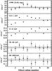 |
Fig. 1 Count rates light curves in different energy ranges. From top to bottom: 2120 Å, 0.5−1 keV, 3−10 keV, 20−60 keV, and 60−200 keV. The horizontal solid lines are the average values and the horizontal dashed lines represent the corresponding ± 1σ uncertainties. |
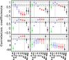 |
Fig. 2 Count rate-count rate correlation coefficients between different energy bands for the 10 observations. In each panel, the green star is the XMM-Newton/OM light curve in the 3−6 eV band; the three blue crosses correspond to the XMM-Newton/pn soft X-ray bands: 0.2−0.5 keV, 0.5−1 keV, 1−2 keV; the three red diamonds correspond to the XMM-Newton/pn medium X-ray bands: 2−4 keV, 4−6 keV, 6−12 keV; and the two black triangles correspond to the INTEGRAL/ISGRI hard X-ray bands: 20−60 keV and 60−200 keV. In each panel, the light curves are correlated with the one marked with the vertical dotted lines. We have overplotted the 95% and 99% confidence levels for the significance of the correlation (it corresponds to correlation coefficients of 0.64 and 0.78, respectively, for 10 points) with horizontal dot-dashed and dashed lines, respectively. |
An important result observed during this campaign is the strong correlation between the UV and soft X-ray (<0.5 keV) flux, while no correlation was found between the UV and the hard (>3 keV) X-rays (see M11). This suggests that the UV and soft X-ray excess variability observed on the timescale of the campaign is produced by the same spectral component, possibly thermal Comptonization (see below).
We have plotted in Fig. 2 the linear Pearson correlation coefficients between light curves in different energy ranges, including those above 10 keV from the INTEGRAL/ISGRI instrument. The error bars reported in this figure were estimated in the following way. To simplify, we focus on the error of the Pearson correlation coefficient of 0.78 obtained between the 3−6 eV and 0.2−0.5 keV count rate light curves. For both energy ranges, we simulated 200 light curves of ten count rates, each of these count rates being drawn from a Gaussian distribution probability centered on the observed values (in these energy ranges) and with a standard deviation equal to the 68% count rate error of the observed data.
We take the example of the simulation of the faked 3−6 eV count rates for Obs. 1. The observed count rate for Obs. 1 is 14.06 cts s-1 with a 90% error of ± 0.76 cts s-1. Thus we draw 200 faked 3 − 6 eV count rates from a Gaussian centered on 14.06 cts s-1 and with a standard deviation of 0.76/1.65 = 0.46 cts s-1. We proceed in the same manner for the 0.2−0.5 keV energy band. Then we correlate the 200 simulated 3−6 eV light curves with the 200 simulated 0.2−0.5 keV light curves to obtain a set of 200 × 200 fake correlation coefficients. We define the correlation coefficient cmin (respectively cmax) as the value below (respectively above) which we have 5% of the simulated correlation coefficients. In the present example, cmin = 0.47 and cmax = 0.85, and we use cmin and cmax as the corresponding 90% error on the observed correlation coefficient. We apply the same procedure for the other correlation coefficients shown in Fig. 2. We have also overplotted, in this figure, the 95% and 99% confidence levels for the significance of the correlation. This correspond to correlation coefficients of 0.64 and 0.78, respectively, for 10 points.
Figure 2 shows that the UV and soft X-rays (<1 keV) bands are indeed well correlated even if the errors on the correlation coefficient are relatively large. But, in contrast, the absence of correlation with the higher energy bands points to separated components between the low (<1 keV) and high (>1 keV) energies. Noticeably, the XMM-Newton energy bands above ~2 keV appear to vary in unison, and also correlate well with the 20−60 keV INTEGRAL energy band, suggesting a common physical origin.
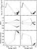 |
Fig. 3 First (left panels) and second (right panels) principal components of variability. The upper panels show the spectra corresponding to the maximal and minimal coordinate αj,k over the j = 10 observations of the first (k = 1, left) and second (k = 2, right) eigenvectors. The middle panels show the ratio of the maximum and minimum spectra to the total spectrum of the source. The bottom panels show the contribution of each component to the total variance as a function of energy. |
4. Principal component analysis
Before going deeper into the spectral analysis, we perform a principal component analysis (PCA) to search for variability patterns. PCA is a powerful tool for multivariate data analysis which is now widely used in astronomy (e.g. Paltani & Walter 1996; Vaughan & Fabian 2004; Malzac et al. 2006; Miller et al. 2007; Pris et al. 2011). It allows transforming a number of (potentially) correlated variables into fewer uncorrelated variables called principal components. In the present case, the long exposures per observation enable the use of a large number of energy bins without being limited by the Poisson noise. We choose a number of 91 energy bins, from the UV (6 bins) up to the X-rays (85 bins), with the INTEGRAL data left out due to their low statistics. Consequently, we have p = 10 spectra obtained at different times t1, t2, ..., tp, and binned into n = 91 energy bins Ei = 1,n. Thus we have a p × n matrix F whose coefficients are given by the energy fluxes of each spectrum in each energy bin. The PCA gives the eigenvalues and eigenvectors Vk = 1,n(E) of the correlation matrix of F, thus defining a new coordinate system that best describes the variance in the data. The observed spectra F(E,tj) can be decomposed along the eigenvectors with a given set of coordinates αk following 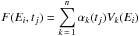 for each energy bin Ei = 1,n. The coordinates αk vary from observation to observation and their fluctuations account for the observed variance. On the contrary, the eigenvectors are constant and define the different variability modes of the set of observations.
The first PCA components are those that reproduce most of the observed variability, with the others dominated by the statistical noise in the data. We have plotted the two first principal components of our analysis in Fig. 3. The first component (left panels of Fig. 3) consists mainly in a variability mode dominated by flux variations in the hard energy range (>1 keV). Most of the sample variance (>87%) is produced by this component. The second PCA component (right panels of Fig. 3) is dominated by variability below 1 keV, and represents 10% of the total variance. The 4% of variance left is distributed between the higher order components not shown here. This result nicely supports the idea that two main components are dominating the broad-band variability of this campaign, one in the UV-soft X-rays and the other in the hard X-rays.
5. Spectral analysis
Here we study the spectral energy distribution between the optical, UV, X-ray, and gamma-ray bands for Mrk 509. The XMM-Newton/pn spectra have been rebinned in order to have a minimum of 25 counts per bin and three bins per resolution element. The cross calibration normalization between XMM-Newton and INTEGRAL is fixed to one. All spectral fits were performed using the xspec software (version 12.3.0). In Sect. 5.1, the reported errors are at the 90% confidence level for one interesting parameter, while in Sect. 5.2, owing to the potential strong correlations between the model parameters, the reported errors are at the 90% confidence level for two interesting parameters.
5.1. Above 3 keV
We first concentrate our analysis on the data above 3 keV, i.e. on a domain known to be dominated by the primary continuum. This agrees with the PCA analysis (Sect. 4), which suggests that a unique component dominates the variability in this energy range. In this section, we are interested in the global spectral behavior of the source. We thus simply use a cut-off power-law for the continuum. More realistic Comptonization models are used in Sect. 5.2 when the broad-band UV/X-rays/gamma-rays energy range is used.
To start, we analyze the total spectrum over the entire campaign to determine the best model components to be used. Afterwards we apply the corresponding model to the different observations in Sect. 5.1.2.
5.1.1. The total spectrum
The best fit and data/model ratio of the total spectrum are plotted in Fig. 4. It clearly shows the presence of an iron line near 6.4 keV. The presence of a high-energy cut-off is not required by the data, and a value below ~200 keV is even excluded at the 90% confidence.
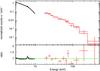 |
Fig. 4 Top: total XMM-Newton (pn, black) and INTEGRAL (ISGRI, red) data above 3 keV. The solid line is the best-fit power-law model. Bottom: ratio data/model. The iron line is clearly visible and no high-energy cut-off is required. |
The iron line complex observed during our campaign is discussed in detail in P12. It can be decomposed into a narrow core (σ ≃ 0.03 keV) and a broader component (σ ≃ 0.22 keV). When looking to archival (XMM-Newton, Chandra, and Suzaku) data, the narrow core appears to be constant on a several-year timescale, peaking at an energy consistent with 6.4 keV. This suggests an origin in remote neutral material (see also De Rosa et al. 2004; Ponti et al. 2009). On the contrary, the intensity of the broader component seems to follow the variations of the continuum throughout the campaign (i.e. on a timescale of a few days), without a measurable time lag (see Fig. 4 of P12). Given the sampling of our monitoring, this suggests an origin within a few light days from the black hole, the width of the line being compatible with a Keplerian motion at 40–1000 gravitational radii from the 1.4 × 10⁸ M⊙ supermassive black hole of Mrk 509. Note that the relatively large EW of ~ 50 eV of this component suggests that part of it could originate in the inner BLR (Costantini et al., in prep.)
Best-fit parameters when fitting the data above 3 keV.
Following P12, we fit the iron line profile with two model components. For the narrow core we used the pexmon model of xspec (Nandra et al. 2007). It reproduces the reflection component following the pexrav model (Zdziarski & Coppi 1991) of xspec, but in addition it includes the Kα and Kβ neutral iron line, the Compton shoulder, and the nickel Kα line, all these components being computed “self-consistently” according to George & Fabian (1991) simulations. We fixed the inclination angle to 30 deg in pexmon. Since it is supposed to model remote reflection, the illuminating spectrum should be an average of the different states of the central source. Thus, we chose to fix the illuminating power-law photon index to 1.9 and a fixed high-energy cut-off at 300 keV. The exact values of these parameters have no significant effects on the results shown in this paper. We let only the normalization of pexmon free to vary in the fit of the total spectrum. Concerning the broader component we used a simple Gaussian whose energy, flux and width are left free to vary during the fit.
The best-fit parameter values for the total spectrum are reported in the first row of Table 1. The power-law photon index Γ = 1.74 ± 0.01, the broad line component peaks at 6.58 ± 0.04, and has an EW of 55 ± 20 eV and the pexmon normalization is Npexmon = (2.9 ± 0.3) × 10-3. The pexmon normalization is mainly constrained by the intensity of the core of the narrow iron-line component. The fit is not satisfactory (χ2/d.o.f. = 468/243), mainly due to the residuals at low energies (close to 3 keV) and possibly due to the influence of the soft X-ray excess.
5.1.2. Individual observations
We applied the same fitting procedure to the ten different observations. The only varying parameters are the photon index and normalization of the power law and the high-energy cut-off and the characteristics (energy, width, and intensity) of the broad-line component. The pexmon normalization is not expected to vary during the campaign (as the signature of remote reflection) and is fixed to the best-fit value obtained with the total spectrum.
The best-fit parameters for each pointing are reported in Table 1. For the individual pointings, we always obtained an acceptable fit. The best-fit photon index is only marginally variable with a range in between 1.68 and 1.77, and the presence of a high-energy cut-off is never required. The shape of the high-energy spectra of Mrk 509 thus changes only slightly during the monitoring. The broad-line component is always statistically needed. The line equivalent width is consistent with a constant with an average value of 55 ± 10 eV. The line flux follows the continuum flux variability, in agreement with the results obtained by P12. However, its energy is only marginally consistent with the 6.4 keV neutral energy, possibly indicating the presence of ionized iron (see P12 for a more detailed discussion).
5.2. From UV to hard X-rays/soft gamma-rays Comptonization models
By fitting above 3 keV we ignore the spectral complexity of the soft X-ray range where soft X-ray excess and warm-absorber (WA) features are present. These spectral features have to be included in the fitting procedure of the whole dataset from UV to hard X-rays/soft gamma-rays. They are discussed in some detail in the next paragraphs.
It is worth noting, at this stage, that the purpose of the present paper is not to test different models (especially concerning the soft X-ray excess or the primary continuum). We instead make the choice of fiting a few, physically motivated spectral components, which will permit us to discuss the corresponding physical interpretation of the data in depth.
5.2.1. The model components
The warm absorber:
the WA has been comprehensively analyzed by Detmers et al. (2011), and we refer the reader to this article for more details. We produced a table from the best model of the WA derived from this analysis and included this table in xspec.
The soft X-ray excess:
as already explained in the introduction, different models exist in the literature to interpret this component. The most commonly used in the last few years are blurred ionized absorption or reflection and warm Comptonization. That no evidence for changes in the X-ray WA was found in Mrk 509 despite a soft X-ray intensity increase of ~60% in the middle of our campaign (Kaastra et al. 2011) disfavors ionized absorption as the origin of the optical-UV/soft X-ray correlation.
Concerning ionized reflection, it is known to be able to produce a soft X-ray excess (Crummy et al. 2006; Ponti et al. 2009; Cerruti et al. 2011; Noda et al. 2011). Moreover, since part of the X-ray emission is reprocessed in opt-UV in the disk, we also expect some correlation between these energy bands. Two arguments weaken, however, the importance of ionized reflection in the opt-UV/X-ray variability behavior observed in Mrk 509. First we expect a reflection bump peaking near 10 keV that should vary with the soft part of the reflection. But no correlation is observed between the soft and the hard X-ray bands (see Fig. 2). It is true, however, that this could be partly explained by the low statistics above 10 keV. But more importantly, part of the iron line should also be produced by this reflection component and would be expected to vary with the soft X-rays. However, neither the narrow core of the line nor its broader component show variations that agree with those observed in the soft X-rays (see Sect. 5.1.1).
Following M11, we chose to model the UV-soft X-ray emission by thermal Comptonization. We used the nthcomp model of xspec. nthcomp covers a wide range of parameters and is well adapted to warm (kT ~ 1 keV)1 and optically thick (τ ~ 10–20) plasma (i.e. what we call a warm corona in the following), such as the one expected to reproduce the steep soft X-ray emission. The free parameters of nthcomp are the temperature of the corona kTwc2, the soft-photon temperature Tbb,wc, and the asymptotic power-law index Γwc of the spectrum. We prefer to use this model instead of comptt (which is similar to the comt model in spex used by M11), because the seed photons in comptt only have a black-body distribution. With nthcomp we can choose a multicolor-disk distribution. It is also fast to use in xspec (see also Appendix A for a comparison of these two models).
Best-fit parameters of the total spectrum and the different observations using the Comptonization model compps for the primary continuum and nthcomp for the UV-soft X-rays.
Note however that nthcomp does not provide the corona optical depth directly. It has to be deduced in another manner, generally by comparing its spectral shape to another model that provides the optical depth. This is, however, a possible source of uncertainties and is discussed in detail in Appendix A. In the following, the optical depth of the warm corona is deduced from a comparison with the eqpair model.
The primary continuum:
concerning the high-energy continuum, the cut-off power-law model is known to be a poor approximation of realistic thermal Comptonization models. First, the high-energy cut-off shape of Comptonization spectra differs from an exponential cut-off. Besides, Comptonization spectra result from the sum of multiple bumps, each one corresponding to the different Compton scattering orders experienced by the soft seed photons in the corona. For small optical depth, the spectral shape is bumpy. Finally, Comptonization spectra naturally include the seed photons that cross the corona but are not Compton-scattered (the so-called zeroth scattering order).
We used the Comptonization model compps (Poutanen & Svensson 1996) of xspec to model the high-energy primary continuum. compps is well adapted to reproducing the emission of a hot and optically thin plasma, i.e., what we call the hot corona in the following. The fit parameters of compps are the temperature of the corona kThc3, either the optical depth τhc or the parameter  , where yhc is equivalent to the Compton parameter for small (<1) optical depths, the temperature of the soft photons produced by the cold phase kTbb,hc (also assuming a multicolor-disk distribution) and the geometry of the disk-corona configuration.
We prefer to use the Compton parameter instead of the optical depth in the fitting procedure to minimize the model degeneracy. Indeed, the temperature and optical depth are generally strongly correlated in the fitting procedure, with the same 2 − 10 keV slope obtained with different combinations of these two parameters (see e.g. Petrucci et al. 2001). We also assume a slab geometry for the corona-disk system.
The iron line:
following the results obtained in Sect. 5.1, we use pexmon to fit the narrow core of the iron line and a Gaussian to fit a broad-line component if needed.
It is important to point out that no link between the Comptonized spectrum and the soft UV emission is imposed a priori. The model simply adjusts its parameters, independently of each other, to fit the data. It is only a posteriori that the resulting best-fit values can be interpreted in a physically motivated scenario.
5.2.2. The COS-FUSE data set
The use of non-simultaneous optical-UV to hard X-ray data could produce spurious constraints on Comptonization models and should be avoided; however, a few arguments make the use of the COS and FUSE data in our spectral analysis reasonable. First, the UV continuum shape of Mrk 509 did not change significantly, even for a 60% lower flux as observed with FOS (Kriss et al. 2011). This suggests that the UV spectral shape of Mrk 509 only weakly changes as its flux varies. Moreover, some of the Swift data were obtained simultaneously with the COS observations in a bandpass comparable to the OM bands. The Swift fluxes are at values comparable to OM points near the beginning and the end of the XMM-Newton campaign, and only 12% below the mean flux of the whole campaign (Kriss et al. 2011). Given the lack of evidence for variation in the spectral shape and the fact that only a small-scale factor is needed to bring the COS data in line with the mean OM fluxes, we decided to use of the COS data in our fit procedure.
The scaling factor to match the FUSE data with the OM one, still assuming a constant spectral shape, is much larger (~2, see M11 for more information on the method used to rescale the COS and FUSE data) and the use of the FUSE data is more arguable. However, it allows for a better constraining of the maximum of the UV bump. For these different reasons, we chose to include the COS and FUSE data in our spectral analysis.
5.2.3. The total spectrum
First, we assume the same soft-photon temperatures for the two Comptonization models, i.e., Tbb,hc = Tbb,wc. The fit is very bad with χ2/d.o.f. = 8850/691, and the data/model ratio shows several features in the X-rays. Relaxing the constraint of equal soft temperatures between the two plasmas enables us to reach a much better fit with χ2/d.o.f. = 1387/690. The corresponding best-fit parameter values are reported in the first row of Table 2. We have plotted in Fig. 5 the corresponding unfolded best-fit model.
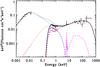 |
Fig. 5 Unfolded best-fit model of the total data spectrum using a thermal Comptonization component (compps in xspec) for the primary continuum. The data are the black crosses. The solid black line is the best-fit model including all absorption (WA and Galactic). The dashed lines correspond to the different spectral components, hot (in red) and warm (in blue) corona emission as well as the reflection (magenta) produced by pexmon including the effects of absorptions, while the dotted line are absorption free. |
The two plasmas clearly have different characteristics. The warm corona is optically thick with τwc ~ 20, a temperature kTwc on the order of 600 eV and a soft-photon temperature Tbb,wc ~ 3 eV. In contrast, the hot corona is optically thin τhc ~ 0.6, with a temperature kThc of about 100 keV and a soft-photon temperature Tbb,hc ~ 100 eV.
In this model, the optical/UV data are entirely fitted by the low-energy part of the warm plasma emission (see Fig. 5). The soft-photon bump of the hot corona, instead, peaks in the soft X-ray range and contributes to the soft X-ray excess. The soft-photon temperature of ~100 eV suggests that the hot corona is localized in the inner region of the accretion flow compared to the warm corona; however, a 100 eV temperature is large for a “standard” accretion disk around a ~108 M⊙ black hole. This point is discussed in Sect. 6.2.1.
The value of 100 keV for the hot corona temperature is compatible with the lower limit on the high-energy cut-off Ec > 200 keV obtained when fitting with a cut-off power-law shape for the primary continuum (see Sect. 5.1). Indeed, as said in the introduction, the cut-off spectral shape of a Comptonization spectrum differs from an exponential cut-off and, roughly speaking, Ec is generally about a factor 2 or 3 larger than the “real” corona temperature. Thus Ec > 200 keV agrees with a corona temperature of ~100 keV.
The fit of the total spectrum is still statistically not acceptable, however, with the presence of strong features in the data/model ratio, especially in the soft X-rays. The FUSE points are also slightly below the best-fit model (see Fig. 5). A possible reason for these discrepancies, given that the fits are reasonably good for each individual observation (see next section), could be the source spectral variability. The total spectrum is then a mix of different spectral states that cannot be easily fit with “steady-state” components.
5.2.4. Individual observations
We repeated the same fitting procedure for the ten different observations, letting Tbb,hc and Tbb,wc free to vary independently. As in Sect. 5.1.2, the pexmon normalization is fixed to the best-fit value obtained with the total spectrum. The best-fit parameters for each pointing are reported in Table 2. The 90% contour plots of the temperature vs. the optical depth are plotted in Fig. 6 for both coronae and for the ten observations. The errors reported in Table 2 are computed from these contour plots and not from the error command of xspec. Indeed, the shape of the χ2 surface is relatively complex for the models used, and confidence intervals are found better by determining the locus of constant Δχ2 than by the use of the error command.
The time evolutions of the different best-fit parameters are plotted in Fig. 7. For each parameter we have overplotted their weighted average value with the corresponding ± 1σ uncertainties. All the light curves are inconsistent with a constant at more than 99% confidence except for the temperature, optical depth, and soft photon temperature of the warm corona.
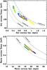 |
Fig. 6 Contour plots of the temperature versus optical depth for the hot (top) and warm (bottom) corona for the 10 observations. We have overplotted the predicted relationship τ vs. kT in steady state assuming a soft-photon temperature of 10 eV and for different Compton amplification ratios: dotted line: Ltot/Ls = 2; dashed line: Ltot/Ls = 3; dot-dot-dot-dashed: Ltot/Ls = 11. |
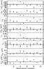 |
Fig. 7 Time evolution of the different fit parameters. From top to bottom: the hot corona temperature kThc, Compton parameter yhc, optical depth τhc, and the warm corona temperature kTwc, photon index Γwc, optical depth τwc, and the soft photon temperatures Tbb,wc and Tbb,hc. The solid lines show the best-fit constant values and the solid lines the ± 1σ uncertainties. |
5.2.5. Heating and cooling
We call Ltot the total corona luminosity and Ls the intercepted soft-photon luminosity, i.e., the part of the soft-photon luminosity emitted by the cold phase that effectively enters and cools the corona. The difference Ltot − Ls then corresponds to the intrinsic heating power provided by the corona to comptonize the seed’s soft photons. The ratio Ltot/Ls is called the Compton amplification ratio.
From our best fits obtained for each observation, we can estimate the seed’s soft-photon luminosity Ls that enters both coronae. Indeed, the number of photons is conserved in the Comptonization process. Consequently, from the number of photons measured in our nthcomp and compps model components and the temperature of the soft-photon field, we can deduce (assuming a multicolor-disk distribution) the corresponding soft-photon luminosity that crosses and cools each corona (see Appendix B). In this reasoning, we assume that no extra component participates in the observed opt-UV emission apart the Comptonization spectra. Any extra component would decrease the effective seed soft-photon luminosity Ls, implying that our estimates of Ls are strict upper limits.
The total corona luminosity Ltot can be deduced from the observed luminosity Lobs of each Comptonization model component and Ls by the relation Ltot ≃ 2Lobs − Lse − τ (see Appendix B), where τ is the corona optical depth. This relation assumes that the corona emissions are isotropic.
We have plotted the values of Ls and Ltot for both coronae, as well as the amplification ratios for the ten observations, in Fig. 8. The errors on Lobs and Ls (and consequently on Ltot) were estimated, in the case of Obs. 1, from a large number of coronae model parameters (kTwc, Γwc, kThc, yhc and the model normalizations), taking into account their likelihood given by the contour plots shown in Fig. 6. The corresponding flux histograms were fitted by a Gaussian from which the 90% error is deduced. These errors are on the order of 5% for Lobs and Ls. Because this procedure is time-consuming, we assume the same order of magnitude for the errors for all the observations.
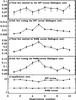 |
Fig. 8 a) Total flux Ltot/LEdd emitted by the hot corona and b) intercepted soft photon luminosity Ls/LEdd entering and cooling the hot corona. c) and d), like a) and b) but for the warm corona. e) Compton amplification ratio Ltot/Ls for the warm (bottom curve) and hot (top curve) coronae, respectively. The dotted line in e) is the expected value for a thick corona in radiative equilibrium above a passive disk. All the luminosities are in Eddington units assuming a black-hole mass of 1.4 × 10⁸ M⊙. The error bars on Lobs and Ls have been estimated as on the order of 5%. |
While the total flux emitted by the hot corona varies during the monitoring, with a significant decrease between Obs. 3 and 4, its variation is limited to about 25%. This is smaller than the variation in its seed soft-photons luminosity, which reaches a maximum in Obs. 5, 70% higher than the luminosity at the beginning or the end of the monitoring. Concerning the warm corona, Ls and Ltot vary similarly, also reaching their maximum in Obs. 5, but ~35% higher than the luminosities estimated in Obs. 1 and 10.
The warm and hot coronae have clearly different amplification ratios (see Fig. 8e). This is remarkably constant and equal to ~2 for the warm plasma as expected given its large optical depth (see Eq. (B.14)) and in between 5−15 for the hot corona, with a significant decrease between Obs. 3 and 6.
6. Discussion
6.1. The disk-corona geometry
As already said in Sect. 5.2, no link between the comptonised spectrum and the soft UV emission is imposed a priori in our fitting procedure. The model simply adjusts its parameters to fit the data. We can, however, compare our best-fit values to theoretical expectations and constrain our own scenario.
The spectral shape of Comptonization models depends on the temperature and optical depth of the corona. Another important parameter is the geometry of the disk-corona system, which can be related to the amplification ratio. In steady states, the corona temperature adjusts, for a given optical depth, to keep this ratio to a constant value. For instance, in the case of a plane-parallel corona geometry in thermal equilibrium above a passive disk, this amplification ratio is expected to be on the order of 3 for a thin (τ < 1) corona and 2 in the thick case (e.g. Haardt & Maraschi 1991 and see Appendix B). Then, photon-starved (respectively photon-fed) geometries, i.e. geometries where the corona is undercooled (respectively overcooled) compared to the plane geometry, have amplification ratios higher (respectively lower) than these theoretical values.
We have overplotted in Fig. 6 the predicted relationships in steady state between the temperature and the optical depth assuming a soft-photon temperature of 10 eV and different Compton amplification ratios. In agreement with the estimated amplification ratios plotted in Fig. 8e, the disk-hot corona system is clearly in a “photon-starved” configuration, with amplification ratios above 3. This suggests a disk-corona geometry where the solid angle under which the corona “sees” the accretion disk is small. This is a common result for Seyfert galaxies. Indeed, the slab geometry cannot reproduce hard X-ray spectra (Γ2−10 < 2) like those observed in Seyfert galaxies because of the strong cooling that is expected from the accretion disk in such geometry (e.g. Haardt 1993; Haardt et al. 1994). A photon-starved disk-corona configuration means less cooling compared to the slab geometry hence harder spectra.
In contrast, the warm corona agrees very well with a configuration of an optically thick plasma covering a passive disk. This is the direct consequence of a large optical depth (τwc ≫ 1) and our assumption to fit the Opt-UV and soft X-ray data with a unique Comptonization component (see Eq. (B.14) with no disk intrinsic emission). The slight disagreement, in Fig. 6, of the predicted relationship in steady state Ltot/Ls = 2 and the contours of the temperature vs. the optical depth comes from the fact that the theoretical prediction, correct for optically thin media, is slightly incorrect at high optical depth.
6.2. The physical origin of the warm and hotcoronae
The sum of the seed soft-photons luminosities Ls,wc + Ls,hc (dominated by Ls,wc ) crossing both coronae is on the order of ~1045 erg s-1 for the total spectrum. Assuming that it is produced by a multicolor accretion disk around a super-massive black hole of 1.4 × 10⁸ M⊙, with an inner-disk radius of 6 Rg (Rg the gravitational radius associated to the black hole) and an inclination angle of 30 degrees, its expected inner-disk temperature should be on the order of 15–20 eV. This is significantly more than the soft-photon temperature ~3 eV of the warm corona but significantly less than the soft-photon temperature ~100 eV of the hot corona.
With the same reasoning, the soft-photon temperature of ~3 eV of the warm corona corresponds to a disk radius of ~30 Rg. Given the expected slab geometry of the disk-warm corona system, it suggests that the warm corona is preferably located at this distance on the disk. On the other hand, the high temperature of the hot corona and the temperature of ~100 eV of its seed soft photons suggest a hot plasma in the inner region of the accretion flow.
6.2.1. warm corona: the disk surface layer?
That we manage to fit the Opt-UV and soft X-ray data with a unique Comptonization component of large optical depth implies an amplification ratio of the warm corona equal to 2 (see Eq. (B.14)), i.e., the theoretical value expected in the case of a thick corona above a passive disk. This strongly suggests that the regions of the accretion disk responsible for the optical-UV emission, which acts as the source of seed photons for the warm plasma, are essentially heated by the warm plasma itself.
With an optical depth of ~20 and a temperature of 500−600 eV, this (plane) warm corona could be seen as the warm skin layer of the accretion disk. In this case the soft emission peaking at 3 eV would come from regions deeper in the disk and heated by the warm layer. Such vertical stratification of the disk is clearly expected in the case of irradiated accretion disks, the upper layer being heated to the Compton temperature of the illuminating flux (e.g. Nayakshin et al. 2000; Nayakshin 2000; Ballantyne et al. 2001b; Done & Nayakshin 2001).
The optical depth of ~20 deduced from our fits appears, however, to be well above the expected theoretical values, on the order of a few units. This could be explained by the very simple assumptions of our corona models, which assume a constant temperature and optical depth for the whole corona. The inclination of the accretion disk could also play a role, since it would increase the effective optical depth compared to the theoretical estimates, which are computed in the vertical direction of the layer.
A natural origin of the illuminating radiation producing the warm corona could be the hot corona itself (see next section). However, the hot corona luminosity is about a factor 2 lower than the total warm corona luminosity (see Fig. 8), so irradiation is only part of the heating mechanism of the upper layers of the accretion disk forming the warm corona. Besides, the amplification ratio of 2 disfavors intrinsic emission produced by the disk deeper layers but instead suggests that the warm corona has its own heating process. If this interpretation is correct, it means that the accretion heating power is most likely to be liberated at this disk surface layer and not in the disk interior. Interestingly, recent 3D radiation-MHD calculations, when applied to protostellar disks, show that the disk surface layer can indeed be heated by dissipating the disk magnetic field, while the disk interior is “magnetically dead” and colder than a standard accretion disk (Hirose & Turner 2011). The same processes could occur in the disk of Mrk 509, giving birth to the warm corona needed in our fits.
It is worth noting, however, that these conclusions are model-dependent, and for instance, they strongly depend on our assumption to fit the optical-UV and soft X-ray emission with a unique Comptonization component. The addition of a pure multicolor-disk component in the optical-UV band would necessarily decrease the importance of the warm corona emission in this energy range and consequently would decrease its amplification ratio. From a statistical point of view, there is no need to add such a multicolor disk component, and thus, with this limit in mind, we can conclude that the warm corona likely covers and heats a large part of the accretion disk.
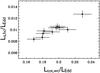 |
Fig. 9 Correlation of the seed soft-photon luminosity of the hot corona, Ls,hc, and the total luminosity of the warm plasma Ltot,wc. |
6.2.2. hot corona: the hot inner flow?
The total power emitted by the hot corona is on the order of 1.3 × 1045 erg s-1 i.e. ~ 5% of the Eddington luminosity of a supermassive black hole of 1.4 × 10⁸ M⊙. There are a few theoretical models that explain the presence of such hot thermal plasma at such high luminosity: for instance the luminous hot accretion flow (LHAF) proposed by Yuan (2001) which is an extension of the ADAF solutions to high accretion rate (see also Yuan et al. 2006). Jet emitting disks (JED) solutions (Ferreira et al. 2006) also provide a hot and optically thin plasma. Since no powerful and collimated jet is observed in Mrk 509, the JED solution is apparently not appropriate. Aborted jets have been proposed, however, to explain the properties of Seyfert galaxies (Henri & Petrucci 1997; Petrucci & Henri 1997; Ghisellini et al. 2004). A JED could then be present but without filling all the conditions for producing a “real” jet, such as its insufficiently large radial extension. The hot corona could be present but not the jet.
The 100 eV temperature for the soft seed photons of the hot corona is a factor ~5 above the value expected from a standard accretion disk. A few physical arguments could help to solve this inconsistency. First, the disk spectra are certainly more complex than the simple sum of blackbodies due to the possible effects of electron scattering in comparison to absorption. Special and general relativistic effects could also play a significant role on the observed emission. These effects lead to modified black-body spectra with an “observed” temperature higher than the effective temperature by a factor between 2 and 3 (e.g. Czerny & Elvis 1987; Ross et al. 1992; Merloni et al. 2000). The presence of the warm corona above a large part of the disk can also strongly modify the disk emission, as shown in our fits (Czerny & Elvis 1987; Czerny et al. 2003; Done et al. 2012).
An interesting interpretation could be that the seed soft photons of the hot corona are those emitted by the warm plasma. The warm plasma emission peaks at a few eV and extends to a few 100’s of eV, so it can be “seen” by the hot corona as a soft photon field with an intermediate temperature of ~100 eV. Such an interpretation cannot be modeled easily with xspec, but it is nicely supported by the strong correlation (with a linear Pearson correlation coefficient equal to 0.92, which corresponds to a >99% confidence level for its significance) between the seed soft photon luminosity of the hot corona, Ls,hc, and the total luminosity of the warm plasma Ltot,wc (see Fig. 9).
6.2.3. A tentative toy picture
From the above discussions, a tentative toy picture of the overall configuration of the very inner regions of Mrk 509 could be the following: a hot corona (Te ~ 100 keV, τ = 0.5) fills the inner part of the accretion flow, below say Rin. It illuminates the outer part of the disk and contributes to the formation of a warm upper layer (Te ~ 1 keV, τ = 20) on the disk beyond Rin, the warm corona. This warm corona also possesses its own heating process, potentially through dissipation of magnetic field at the disk surface. It heats the deeper layers of the accretion disk, which then radiates like a black body (at Tbb ~ 3 eV). This warm corona upscatters these optical-UV photons up to the soft X-ray, a small part of them entering and cooling the hot corona. The small solid angle under which the hot flow sees the warm plasma agrees with the large amplification ratio of ~5−10 estimated from our fits. The 100 eV temperature obtained by our xspec modeling would be explained by the fact that xspec would try to mimic the warm plasma emission, which covers an energy range between ~1 eV and ~1 keV, with the multicolor-disk spectral energy distribution of the seed soft photons available in compps. A tentative sketch is shown in Fig. 10.
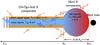 |
Fig. 10 A sketch of the accretion flow geometry in the inner region of the galaxy Mrk 509. The hot corona, producing the hard X-ray emission, has a temperature of ~100 keV and optical depth ~0.5. It is localized in the inner part of the accretion flow (R < Rin) and illuminates the accretion disk beyond Rin, helping to form a warm layer at the disk surface. This warm component has a temperature of ~1 keV and an optical depth ~15 and produces the optical-UV up to soft X-ray emission. It extends over a large part of the accretion flow, heating the deeper layers and comptonizing their optical-UV emission. In return, part of this emission enters and cools the hot corona. |
Clearly, in this picture the two coronae should be powered by the same accretion flow and should consequently be energetically coupled. Assuming that the warm corona covers the accretion disk between Rout and Rin and then that the hot corona fills the space between Rin and Risco, then the accretion power liberated in the warm corona is ![\begin{equation} P_{\rm acc,wc}=\frac{GM\dot{M}}{2R_{\rm in}}\left [1-\frac{R_{\rm in}}{R_{\rm out}}\right ], \label{eq1} \end{equation}](/articles/aa/full_html/2013/01/aa19956-12/aa19956-12-eq230.png) (1)while the accretion power liberated in the hot corona is
(1)while the accretion power liberated in the hot corona is ![\begin{equation} P_{\rm acc,hc}=\frac{GM\dot{M}}{2R_{\rm isco}}\left [1-\frac{R_{\rm isco}}{R_{\rm in}}\right ], \label{eq2} \end{equation}](/articles/aa/full_html/2013/01/aa19956-12/aa19956-12-eq231.png) (2)so the ratio between the two is
(2)so the ratio between the two is 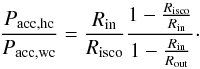 (3)Neglecting the advection, which seems reasonable given the accretion rate of the system, the accretion power liberated in each corona is close to their total luminosity. The ratio Pacc,hc/Pacc,wc is then on the order of Ltot,hc/Ltot,wc and Eq. (3) gives a one-to-one relationship between the total luminosities Ltot,hc and Ltot,wc (or, equivalently, Ltot,hc and Ltot,hc/Ltot,wc) and the inner disk radius Rin and total accretion rate Ṁ, as soon as Risco and Rout are given.
We have mapped, in Fig. 11, the Rin − Ṁ plane into the Ltot,hc − Ltot,hc/Ltot,wc plane assuming Risco = 6 Rg and Rout = 100 Rg. The observed total luminosities agree with Eqs. (1) and (2) if Rin is between 8 and 10 Rg and the accretion rate Ṁ between 20 and 30% of the Eddington rate (assuming an accretion efficiency η = (2 Risco/Rg)-1). Rin strongly depends on Risco and decreases as Risco decreases. A value of 10 Rg can then be seen as a rough upper limit. On the other hand, Ṁ only slightly depends on Risco. Both Rin and Ṁ very slightly depend on Rout unless Rout become very small (<10−20 Rg).
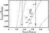 |
Fig. 11 Contour plots of the inner disk radius Rin (solid lines, in units of Rg) and the total accretion rate Ṁ (dashed lines, in Eddington units and assuming an accretion efficiency η = (2Risco/Rg)-1) in the Ltot,hc − Ltot,hc/Ltot,wc plane (see Eqs. (1) and (2)). The points indicate the positions of the 10 observations. |
6.3. A luminosity-independent spectral shape for the soft X-ray excess
That the warm corona, which is at the origin of the Opt-UV to soft X-ray emission in our modeling of Mkr 509, has naturally a constant amplification ratio has an interesting consequence. It implies a spectral emission that is almost independent of the AGN luminosity. Indeed, the photon index of the comptonized spectrum is directly linked to the amplification ratio (e.g. Beloborodov 1999; Malzac et al. 2001). A constant amplification ratio then implies a roughly constant spectral index. This also depends on the soft photon temperature, but this effect is weak as far as this temperature is not varying too much. Moreover, in radiative equilibrium the corona temperature and optical depth follow a univocal relationship. For a given optical depth τ corresponds a unique temperature kT and, to the extent that the radiative equilibrium is insured, there is no reason for τ and kT to vary. The temperature and optical depth of the warm corona are indeed consistent with a constant during the monitoring (see Fig. 7). Thus, in these conditions, we expect an almost constant spectral shape for the soft X-ray excess, regardless of the luminosity of the AGN, in very good agreement with observations (e.g. Gierlinski & Done 2004; Crummy et al. 2006; Ponti et al. 2006).
6.4. Geometry variations
Simulations by Malzac & Jourdain (2001) show that the time scale for a disk-corona system to reach equilibrium, after rapid radiative perturbation in one of the two phases, is of a few corona light crossing times i.e. shorter than a day. We can thus (reasonably) assume that each of the ten spectra of Mrk 509 correspond to a disk-corona system where hot and cold phases are in radiative balance with each other. In this case, a fixed disk-corona configuration in radiative equilibrium should correspond to a constant heating/cooling ratio. As already said, this is what we observe in the case of the warm corona, its amplification ratio being necessarily (given our model) equal to 2 (see Fig. 8e). In the case of the hot corona, however, the amplification ratio decreases in the middle of the campaign (Obs. 4 and 5) suggesting a variation in the disk-hot corona configuration during the monitoring.
A decrease in the amplification ratio means that the disk-hot corona geometry becomes less photon-starved. During Obs. 4 and 5 the total luminosity of the warm corona increases (cf. Fig. 8c), while the total luminosity of the hot corona decreases (cf. Fig. 8a). If the above picture is correct, these variations should be linked somehow to variations in the inner accretion disk radius Rin and/or of the total accretion rate. Looking to Fig. 11, variations of ~5−10% for these parameters are enough to explain the observed luminosity variations. The variation in Rin can also explain the variation in the hot corona amplification factor.
6.5. A pair-dominated hot corona?
From the luminosities Ltot and Ls, we can estimate the compactness ltot = LtotσT/(Rmec3) and ls = LsσT/(Rmec3) where σT is the Thomson cross section, me the electron mass, c the speed of light, and R the typical size of the corona. We assume R = 10 Rg. Then, on average for the 10 observations, the total compactness ltot,hc ~ 100, and the soft compactness ls,hc ~ 15 for the hot corona, while ltot,wc ~ 230 and ls,wc ~ 115 for the warm corona. For such values of ltot and ls (and thus lh = ltot − ls the heating compactness), no pair equilibrium can be reached for the warm corona given its very low temperature (cf. Ghisellini & Haardt 1994, G94 hereafter, and their Fig. 2). This is different for the hot corona, which has a high enough temperature, given its values of ltot and ls, to be dominated by pairs.
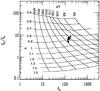 |
Fig. 12 Hard-to-soft compactness ratio lh/ls vs. hard compactness ls. The figure is extracted from Ghisellini & Haardt (1994). It shows the one-to-one correspondence between the spectral characteristics of the Compton spectrum of a pure pair plasma (energy spectral index α and temperature kT) and the soft and hard compactnesses.The black points correspond to the 10 observations of Mrk 509. |
For a pure pair plasma, there is a one-to-one relationship between the hard and soft compactnesses and the spectral characteristics (energy spectral index α and temperature kT) of the Compton spectrum. G94 have mapped the plane α-kT into the plane (lh/ls − lh). We have reported their Fig. 2 in our Fig. 12, overplotting the values of lh,hc and ls,hc computed for the 10 observations of Mrk 509.
Astonishingly enough, given the simple assumptions of the G94 model (homogeneous spherical corona in a homogeneous black body photon field) and our approximated estimates of the compactnesses, they agree nicely with the theoretical expectations of a pure pair plasma. The observed spectral index α ~ 0.7−0.8 (see Table 1, with α = Γ−1), the hot corona temperature on the order of 100 keV, and the variations of these parameters during the monitoring (i.e. Δα ~ 0.1 and ΔkT ~ 80 keV) are not far from the expected ranges. While this comparison is admittedly rough (e.g. the observed spectral index α should have been steeper between 0.8 and 0.9 to completely agree with the expectation), it is interesting to notice that the hot corona behaves spectrally as if it is dominated by pairs.
In the case of a pair-dominated plasma, the increase in the cooling, for a constant heating, is expected to produce an increase in the plasma temperature and not a decrease. This can be seen in Fig. 12. Fixing lh but increasing ls shifts the pair plasma to a higher temperature state. This can be understood as follows (see G94): increasing the cooling first decreases the plasma temperature. But this implies a decrease in the pair creation rate, i.e., a decrease in the number of particles. The available energy is thus shared among fewer particles and eventually, when pair equilibrium is reached again, the temperature is higher.
From our fits, the soft compactness ls,hc of the hot corona varies by ~60% during the monitoring, while the heating compactness lh,hc varies by ~15%. Thus we are roughly in the case of a constant heating with variable cooling. Interestingly enough, the hot corona temperature deduced from our modeling (marginally) correlates with ls,hc as expected for a pair-dominated plasma. The linear Pearson correlation coefficient is equal to 0.67, which corresponds to a 95% confidence for its significance.
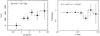 |
Fig. 13 Left: lag energy spectrum. It is obtained by computing time lags in Fourier frequency space, between the energy band 0.3 − 10 keV and a number of adjacent energy channels, averaging the resulting lags over the frequency interval 10-5 − 10-4 Hz. Right: coherence between 0.3−1 and 1−10 keV energy bands as a function of Fourier frequency once a correction for the Poisson noise effects is applied (Vaughan & Nowak 1997). |
6.6. Some hint of the behavior on short time scale?
To investigate the short time scale correlations between spectral components in the X-ray band, we estimated the coherence function (e.g. Vaughan & Nowak 1997) between the 0.3−1 keV and 1−10 keV energy bands by making use of the XMM-Newton data (see right plot of Fig. 13). The two energy bands display a high level of linear correlation over all the sampled frequencies (corresponding to time scales between 60 and 0.5 ks). This behavior is at odds with the observed lack of correlated variability on longer time scales (see Fig. 2 and Sect. 3). However, this result is consistent with the existence of a small and compact hot corona, which is able to produce coherent variations on short time scales.
We explored the causal connection between the different spectral components by computing time lags as a function of energy (see left plot of Fig. 13). The time lags are first computed in the Fourier frequency domain between the entire 0.3 − 10 keVreference band and adjacent channels, with the channel being subtracted from the reference at each step, so as to remove the contribution from correlated Poisson noise (e.g. Zoghbi et al. 2011). The derived lags are then averaged over the range of frequencies Δν ~ 10-5−10-4 Hz, i.e., the frequency domain not dominated by Poisson noise, and plotted as a function of energy. The lag spectrum has been shifted so that the zero-lag energy channel corresponds to the leading one. Hard positive lags (variations in the hard channels being delayed with respect to those in the soft channels) are observed over the full energy band, the relative amplitude of the measured lags increasing with the energy separation between the channels. This trend is commonly observed in black hole X-ray binaries, as well as in some AGNs in the low-frequency range (e.g. Nowak et al. 1999; Papadakis et al. 2001; Arevalo et al. 2006; Zoghbi et al. 2011; Uttley et al. 2011; De Marco et al. 2012).
These hard positive lags are generally interpreted by the propagation of mass accretion rate fluctuations in the disk (e.g. Kotov et al. 2001; Arevalo et al. 2006) and, in order to be observed in the soft X-ray bands, the soft X-ray emitting region has to be strongly connected somehow to the disk accretion flow. This is naturally expected if the soft X-ray emitting region is the upper layer of the accretion disk, as we propose for the warm corona.
6.7. Do we have all the pieces of the puzzle?
Most of our results are model-dependent. For instance, we could add other spectral components (like e.g. a blurred reflection or a pure disk black body) to fit the UV and soft X-rays. The possibilities are numerous and may give a different picture of the inner regions of Mrk 509 than the one revealed by our modeling. Our choice was instead to choose a small number of spectral components. Our main assumption was that the optical-UV emission, observed in the optical monitor of XMM-Newton, was the signature of an optically thick multi-color accretion disk whose optical-UV photons are comptonised in two different media: the first one (the warm corona) producing the soft X-ray excess and the second one (the hot corona) the high-energy continuum emission. In this framework it appears that:
-
The warm corona has an amplification ratio equal to two i.e. the expected value of an optically thick plasma above a passive accretion disk, the disk emission being dominated by the reprocessing. In consequence, most of the disk emission is due to the heating from the warm corona itself. The warm corona could be the warm upper layer of the accretion disk.
-
The hot corona amplification ratio is between five and ten and thus suggests a more photon-starved geometry. The temperature of the soft seed photons entering and cooling the hot corona, on the order of 100 eV, suggests a location in the inner region of the accretion flow.
-
A 100 eV temperature is about a factor 5 above the expected value for a standard accretion disk around a 1.4 × 10⁸ M⊙ black hole. Effects of electron scattering and of special and general relativity could significantly affect the observed emission and lead to modified black body spectra with an “observed” temperature higher than the effective temperature. The seed soft photons of the hot corona can also be part of the warm corona emission. The 100 eV temperature obtained by our xspec modeling would be explained by the fact that xspec would try to mimic the warm plasma emission, which covers an energy range between 3 and ~1 keV, with the multicolor-disk spectral energy distribution available in compps for the seed soft-photon field.
-
The hot corona may be dominated by pairs.
-
The observed flux and spectral variability are mainly due to changes in coronae geometries.
It has been recently suggested by Done et al. (2012) that the accretion disk in AGNs could evolve radially from an optically thick accretion disk beyond a transition radius called Rcorona to a two-phase accretion flow at smaller radii, formed by an optically thick Comptonized disk and an optically thin corona. The latter would play the role of our hot corona, while the optically thick Comptonized disk will produce the warm Comptonized emission. The energetic coupling between the two coronae is taken into account in this model. It possesses the different components used in our fits (the accretion disk and the warm and hot plasmas). However, it assumes that the warm and hot coronae are localized in the same region of the accretion flow, below Rcorona, with the warm corona embedded in the hot one (see Fig. 5 of Done et al. 2012). This picture does not agree completely with our estimates of the amplification ratios; however, it is interesting to see that our conclusions are in broad agreement with the assumptions proposed by these authors. It will be worth testing their model on the Mrk 509 data4. This is devoted to a future work.
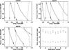 |
Fig. A.1 Contours of the temperature (dashed lines) and optical depth (solid lines) in the Γ-kTnth parameter space of nthcomp for compst (top left), comptt (top right) and eqpair (bottom left) respectively. Bottom right: light curves of the optical depth estimates during the whole campaign for the three models: diamonds: compst, squares: eqpair; triangles: comptt. |
7. Conclusions
Mrk 509 was monitored simultaneously with XMM-Newton and INTEGRAL for one month in late 2009, with one observation every four days for a total of ten observations. A series of papers has already been published using these data focusing on different aspects of the campaign. Here we analyzed the broad-band optical/UV/X-ray/gamma-ray continuum of the source during this monitoring. Our main effort was to adopt realistic Comptonization models to fit the primary continuum, the accretion disk, and the soft X-ray excess.
We obtained a relatively good fit to the data by assuming the existence of two clearly different media: a hot (kT ~ 100 keV), optically-thin (τ ~ 0.5) corona for the primary continuum emission, and a warm (kT ~ 1 keV), optically-thick (τ ~ 10−20) plasma for the optical-UV to soft X-ray emission.
These two media have very different geometries: the warm corona covers a large part of the accretion disk, the disk radiation being dominated by the reprocessing of the warm corona emission. The warm corona could be the warm upper layer of the accretion disk. The temperature of the soft-photon field cooling it is on the order of 3 eV.
In contrast, the hot corona has a more photon-starved geometry and can be the inner part of the accretion flow. The transition radius Rin between the outer disk/warm plasma and the hot inner corona is estimated to be around 10–20 Rg. The variation in Ṁ but also in Rin would be at the origin of the variation in the coronae luminosities, the variation in Rin also producing the variation in the hot corona amplification ratio. The spectral and flux variation in the hot corona are also consistent with a pair-dominated plasma.
These different conclusions may depend at some level on the choice of our modelling. For example, we do not include blurred ionized reflection, while part of the soft X-ray excess could be produced by this component. The presence of an (admittedly weak) ionized iron line, which agrees with a relativistic profile, by P12 would also support the presence of such reflection. On the typical time scale (~day) of this campaign, however, it does not seem to play a major role and Comptonization in a warm plasma, covering the accretion disk, appears the most natural explanation for the soft X-ray excess in Mrk 509.
Acknowledgments
P.O.P. acknowledges the very interesting discussions with J. Ferreira and G. Lesur. This work is based on observations obtained with XMM-Newton, an ESA science mission with instruments and contributions directly funded by ESA Member States and the USA (NASA). It is also based on observations with INTEGRAL, an ESA project with instrument and science data center funded by ESA member states (especially the PI countries: Denmark, France, Germany, Italy, Switzerland, Spain), Czech Republic, and Poland and with the participation of Russia and the USA. This work made use of data supplied by the UK Swift Science Data Centre at the University if Leicester. SRON is supported financially by NWO, the Netherlands Organization for Scientific Research. J.S. Kaastra thanks the PI of Swift, Neil Gehrels, for approving the TOO observations, and the duty scientists at the William Herschel Telescope for performing the service observations. P.-O. Petrucci acknowledges financial support from the CNES and the French GDR PCHE. M. Cappi, M. Dadina, S. Bianchi, and G. Ponti acknowledge financial support from contract ASI-INAF n. I/088/06/0. N. Arav and G. Kriss gratefully acknowledge support from NASA/XMM-Newton Guest Investigator grant NNX09AR01G. Support for HST Program number 12022 was provided by NASA through grants from the Space Telescope Science Institute, which is operated by the Association of Universities for Research in Astronomy, Inc., under NASA contract NAS5-26555. E. Behar was supported by a grant from the ISF. A. Blustin acknowledges the support of an STFC Postdoctoral Fellowship. P. Lubiński has been supported by the Polish MNiSW grants N N203 581240 and 362/1/N-INTEGRAL/2008/09/0. M. Mehdipour acknowledges the support of a PhD studentship awarded by the UK Science & Technology Facilities Council (STFC). G. Ponti acknowledges support via an EU Marie Curie Intra-European Fellowship under contract no. FP7-PEOPLE- 2009-IEF-254279. K. Steenbrugge acknowledges the support of Comité Mixto ESO – Gobierno de Chile.
References
- Arévalo, P., Papadakis, I. E., Uttley, P., et al. 2006, MNRAS, 372, 401 [NASA ADS] [CrossRef] [Google Scholar]
- Beloborodov, A. M. 1999, in High Energy Processes in Accreting Black Holes, ASP Conf. Ser., 161, 295 [NASA ADS] [Google Scholar]
- Cerruti, M., Ponti, G., Boisson, C., et al. 2011, A&A, 535, A113 [NASA ADS] [CrossRef] [EDP Sciences] [Google Scholar]
- Coppi, P. S. 1991, Ph.D. Thesis (Pasadena: California Institute of Technology). [Google Scholar]
- Crummy, J., Fabian, A. C., Gallo, L., & Ross, R. R. 2006, MNRAS, 365, 1067 [NASA ADS] [CrossRef] [Google Scholar]
- Czerny, B., & Elvis, M. 1987, ApJ, 321, 305 [NASA ADS] [CrossRef] [Google Scholar]
- Czerny, B., Nikoajuk, M., Rozanska, A., et al. 2003, A&A, 412, 317 [NASA ADS] [CrossRef] [EDP Sciences] [Google Scholar]
- Dadina, M. 2007, A&A, 461, 1209 [NASA ADS] [CrossRef] [EDP Sciences] [Google Scholar]
- De Marco, B., Ponti, G., Cappi, M., et al. 2012, MNRAS, submitted [arXiv:1201.0196] [Google Scholar]
- De Rosa, A., Piro, L., Matt, G., & Perola, G. C. 2004, A&A, 413, 895 [NASA ADS] [CrossRef] [EDP Sciences] [Google Scholar]
- Deluit, S., & Courvoisier, T. J.-L. 2003, A&A, 399, 77 [NASA ADS] [CrossRef] [EDP Sciences] [Google Scholar]
- Detmers, R. G., Kaastra, J. S., Steenbrugge, K. C., et al. 2011, A&A, 534, A38 [NASA ADS] [CrossRef] [EDP Sciences] [Google Scholar]
- Dewangan, G. C., Griffiths, R. E., Dasgupta, S., & Rao, A. R. 2007, ApJ, 671, 1284 [NASA ADS] [CrossRef] [Google Scholar]
- Done, C., Davis, S. W., Jin, C., Blaes, O., & Ward, M. 2012, MNRAS, 420, 1848 [NASA ADS] [CrossRef] [Google Scholar]
- Ferreira, J., Petrucci, P.-O., Henri, G., Sauge, L., & Pelletier, G. 2006, A&A, 447, 813 [NASA ADS] [CrossRef] [EDP Sciences] [Google Scholar]
- George, I. M., & Fabian, A. C. 1991, MNRAS, 249, 352 [NASA ADS] [CrossRef] [Google Scholar]
- Ghisellini, G., & Haardt, F. 1994, ApJ, 429, L53 [NASA ADS] [CrossRef] [Google Scholar]
- Ghisellini, G., Haardt, F., & Matt, G. 2004, A&A, 413, 535 [NASA ADS] [CrossRef] [EDP Sciences] [Google Scholar]
- Gierlinski, M., & Done, C. 2004, MNRAS, 349, L7 [NASA ADS] [CrossRef] [Google Scholar]
- Gierlinski, M., & Done, C. 2006, MNRAS, 371, L16 [NASA ADS] [CrossRef] [Google Scholar]
- Gondek, D., Zdziarski, A. A., Johnson, W. N., et al. 1996, MNRAS, 282, 646 [NASA ADS] [CrossRef] [Google Scholar]
- Haardt, F. 1993, ApJ, 413, 680 [NASA ADS] [CrossRef] [Google Scholar]
- Haardt, F., & Maraschi, L. 1991, ApJ, 380, L51 [NASA ADS] [CrossRef] [Google Scholar]
- Haardt, F., Maraschi, L., & Ghisellini, G. 1994, ApJ, 432, L95 [NASA ADS] [CrossRef] [Google Scholar]
- Haardt, F., Maraschi, L., & Ghisellini, G. 1997, ApJ, 476, 620 [NASA ADS] [CrossRef] [Google Scholar]
- Henri, G., & Petrucci, P. O. 1997, A&A, 326, 87 [NASA ADS] [Google Scholar]
- Hirose, S., & Turner, N. J. 2011, ApJ, 732, L30 [NASA ADS] [CrossRef] [Google Scholar]
- Jin, C., Done, C., Ward, M., Gierliski, M., & Mullaney, J. 2009, MNRAS, 398, L16 [NASA ADS] [CrossRef] [Google Scholar]
- Jourdain, E., Bassani, L., Bouchet, L., et al. 1992, A&A, 256, L38 [NASA ADS] [Google Scholar]
- Kaastra, J. S., Petrucci, P. O., Cappi, M., et al. 2011, A&A, 534, A36 [NASA ADS] [CrossRef] [EDP Sciences] [Google Scholar]
- Kaastra, J. S., Detmers, R. G., Mehdipour, M., et al. 2012, A&A, 539, A117 [NASA ADS] [CrossRef] [EDP Sciences] [Google Scholar]
- Kotov, O., Churazov, E., & Gilfanov, M. 2001, MNRAS, 327, 799 [NASA ADS] [CrossRef] [Google Scholar]
- Kriss, G. A., Arav, N., Kaastra, J. S., et al. 2011, A&A, 534, A41 [NASA ADS] [CrossRef] [EDP Sciences] [Google Scholar]
- Magdziarz, P., Blaes, O. M., Zdziarski, A. A., Johnson, W. N., & Smith, D. A. 1998, MNRAS, 301, 179 [NASA ADS] [CrossRef] [Google Scholar]
- Maisack, M., Johnson, W. N., Kinzer, R. L., et al. 1993, ApJ, 407, L61 [NASA ADS] [CrossRef] [Google Scholar]
- Malzac, J., Beloborodov, A. M., & Poutanen, J. 2001, MNRAS, 326, 417 [NASA ADS] [CrossRef] [Google Scholar]
- Malzac, J., Petrucci, P. O., Jourdain, E., et al. 2006, A&A, 448, 1125 [NASA ADS] [CrossRef] [EDP Sciences] [Google Scholar]
- Matt, G. 2001, X-ray Astronomy: Stellar Endpoints, AGN, and the Diffuse X-ray Background, AIP Conf. Proc., 599, 209 [NASA ADS] [CrossRef] [Google Scholar]
- Mehdipour, M., Branduardi-Raymont, G., Kaastra, J. S., et al. 2011, A&A, 534, A39 [NASA ADS] [CrossRef] [EDP Sciences] [Google Scholar]
- Merloni, A., Fabian, A. C., & Ross, R. R. 2000, MNRAS, 313, 193 [NASA ADS] [CrossRef] [Google Scholar]
- Middleton, M., Done, C., Ward, M., Gierliski, M., & Schurch, N. 2009, MNRAS, 394, 250 [NASA ADS] [CrossRef] [Google Scholar]
- Miller, L., Turner, T. J., Reeves, J. N., et al. 2007, A&A, 463, 131 [NASA ADS] [CrossRef] [EDP Sciences] [Google Scholar]
- Miller, L., Turner, T. J., & Reeves, J. N. 2008, A&A, 483, 437 [NASA ADS] [CrossRef] [EDP Sciences] [Google Scholar]
- Molina, M., Bassani, L., Malizia, A., et al. 2009, MNRAS, 399, 1293 [NASA ADS] [CrossRef] [Google Scholar]
- Nandra, K., O’Neill, P. M., George, I. M., & Reeves, J. N. 2007, MNRAS, 382, 194 [NASA ADS] [CrossRef] [Google Scholar]
- Noda, H., Makishima, K., Yamada, S., et al. 2011, PASJ, 63, 925 [Google Scholar]
- Nowak, M. A., Wilms, J., & Dove, J. B. 1999, ApJ, 517, 355 [NASA ADS] [CrossRef] [Google Scholar]
- Paltani, S., & Walter, R. 1996, A&A, 312, 55 [NASA ADS] [Google Scholar]
- Papadakis, I. E., Nandra, K., Kazanas, D., 2001, ApJ, 554, L133 [NASA ADS] [CrossRef] [Google Scholar]
- Perola, G. C., Matt, G., Cappi, M., et al. 2002, A&A, 389, 802 [Google Scholar]
- Peterson, B. M., Ferrarese, L., Gilbert, K. M., et al. 2004, ApJ, 613, 682 [NASA ADS] [CrossRef] [Google Scholar]
- Petrucci, P. O., & Henri, G. 1997, A&A, 326, 99 [NASA ADS] [Google Scholar]
- Petrucci, P. O., Haardt, F., Maraschi, L., et al. 2000, ApJ, 540, 131 [NASA ADS] [CrossRef] [Google Scholar]
- Petrucci, P. O., Haardt, F., Maraschi, L., et al. 2001, ApJ, 556, 716 [NASA ADS] [CrossRef] [Google Scholar]
- Petrucci, P. O., Maraschi, L., Haardt, F., & Nandra, K. 2004, A&A, 413, 477 [NASA ADS] [CrossRef] [EDP Sciences] [Google Scholar]
- Ponti, G., Miniutti, G., Cappi, M., et al. 2006, MNRAS, 368, 903 [NASA ADS] [CrossRef] [Google Scholar]
- Ponti, G., Cappi, M., Vignali, C., et al. 2009, MNRAS, 394, 1487 [NASA ADS] [CrossRef] [Google Scholar]
- Ponti, G., Cappi, M., Costantini, E., et al. 2013, A&A, 549, A72 [NASA ADS] [CrossRef] [EDP Sciences] [Google Scholar]
- Pris, I., Petitjean, P., Rollinde, E., et al. 2011, A&A, 530, A50 [NASA ADS] [CrossRef] [EDP Sciences] [Google Scholar]
- Poutanen, J., & Svensson, R. 1996, ApJ, 470, 249 [NASA ADS] [CrossRef] [Google Scholar]
- Ross, R. R., Fabian, A. C., & Mineshige, S. 1992, MNRAS, 258, 189 [NASA ADS] [CrossRef] [Google Scholar]
- Schurch, N. J., Done, C., & Proga, D. 2009, ApJ, 694, 1 [NASA ADS] [CrossRef] [Google Scholar]
- Stern, B. E., Poutanen, J., Svensson, R., Sikora, M., & Begelman, M. C. 1995, ApJ, 449, L13 [NASA ADS] [CrossRef] [Google Scholar]
- Sunyaev, R. A., & Titarchuk, L. G. 1980, A&A, 86, 121 [NASA ADS] [Google Scholar]
- Svensson, R. 1996, A&AS, 120, C475 [NASA ADS] [Google Scholar]
- Titarchuk, L. 1994, ApJ, 434, 570 [NASA ADS] [CrossRef] [Google Scholar]
- Turner, T. J., & Miller, L. 2009, A&ARv, 17, 47 [Google Scholar]
- Uttley, P., Wilkinson, T., Cassatella, P., et al. 2011, MNRAS, 414, L60 [NASA ADS] [Google Scholar]
- Vaughan, S., & Fabian, A. C. 2004, MNRAS, 348, 1415 [NASA ADS] [CrossRef] [Google Scholar]
- Vaughan, B. A., & Nowak, M. A. 1997, ApJ, 474, L43 [NASA ADS] [CrossRef] [Google Scholar]
- Walter, R., & Fink, H. H. 1993, A&A, 274, 105 [NASA ADS] [Google Scholar]
- Yuan, F. 2001, MNRAS, 324, 119 [NASA ADS] [CrossRef] [Google Scholar]
- Yuan, F., Taam, R. E., Xue, Y., & Cui, W. 2006, ApJ, 636, 46 [NASA ADS] [CrossRef] [Google Scholar]
- Zdziarski, A. A., & Coppi, P. S. 1991, ApJ, 376, 480 [NASA ADS] [CrossRef] [Google Scholar]
- Zdziarski, A. A., Lightman, A. P., & Maciolek-Niedzwiecki, A. 1993, ApJ, 414, L93 [NASA ADS] [CrossRef] [Google Scholar]
- Zoghbi, A., Uttley, P., & Fabian, A. C. 2011, MNRAS, 412, 59 [NASA ADS] [CrossRef] [Google Scholar]
Appendix A: Optical depth estimates
The nthcomp model used to fit the optical-UV-soft X-ray emission does not directly provide the value of the optical depth of the plasma for which it models the emission. However, the plasma optical depth has more physical meaning than the photon index of the emitted spectrum, so it is an important parameter that we need to estimate. Generally, one compares the nthcomp spectral shape, for a given set of photon index and temperature, to another model that provides the optical depth. While commonly used, the procedure is generally not precisely discussed. The accuracy of this comparison is important, because inaccurate values for the temperature and optical depth will give a different interpretation for the heating/cooling ratios (see Sect. 6.1).
We compared the results obtained with nthcomp with those from three other xspec Comptonization models: compst, comptt, and eqpair. compst (Sunyaev & Titarchuk 1980) only has the corona temperature and optical depth as free parameters (no parameter for the soft photon temperature), but the range of validity is relatively wide, including low temperature and large optical depth as expected in our case. comptt (Titarchuk 1994) is a commonly used Comptonization code that provides the optical depth and the temperature. Like compst it assumes a black body distribution for the soft photon field. This is the model used by M11. eqpair is a more complete Comptonization model that carefully takes most of the microphysics needed to compute realistic Comptonization spectra into account (Coppi 1991). The soft photon distribution can be either a simple black body or a multicolor disk spectrum. It can treat hybrid thermal/non-thermal particle distributions. Its natural parameters are the optical depth and the heating/cooling ratio. The temperature is an output of the code. To obtain the temperature in xspec, the chatter command has to be larger than 15. However, for most of these models, the values expected for the temperature and optical depth of the warm corona are outside the nominal range of validity indicated in xspec. The temperature has to be between 2 and 500 keV for comptt, between 1 keV and 1 MeV for nthcomp, and the optical depth should be below 10 for eqpair. It is thus interesting to see how these models compare.
We report in Figs. A.1a, b, and c the contours of the temperature and optical depth for the three models compst, comptt, and eqpair in the Γ-kTnth parameter space of nthcomp. We restrict our analysis to low temperatures and steep spectra as expected for the warm corona. While the contours of compst and eqpair look relatively similar, the optical depth estimated with comptt is a factor two smaller. The corresponding optical depth estimates for the ten different observations of Mrk 509 discussed in this paper are plotted in Fig. A.1d. Possible explanations of this difference can be found in the different model assumptions, especially concerning the geometry of the disk-corona systems. It is also worth noting that the best fit temperature values of the warm corona obtained by M11 are significantly lower (by a factor 4) than ours. In this case, however, the main reason for this difference is certainly in the use of a different model for the primary continuum (M11 use a power law). Interestingly enough, while the exact values of the optical depth clearly depend on the model used (cf. Fig. A.1d), its variability throughout the monitoring looks very similar and is apparently independent of the model used.
Appendix B: Estimation of the Ls and Ltot
To estimate the seed soft photon luminosity entering and cooling a corona of optical depth τ, we use the conservation of the number of photons, which characterizes the Compton process. From the observed comptonized spectrum, we deduce an observed photon rate nobs. By conservation, this photon rate is equal to the sum of the seed photons crossing the corona without being comptonized ns,0 and those comptonized in the corona and emitted upward (in direction to the observer) nc,up. At first order, 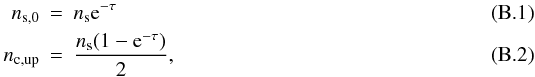 the factor 1/2 of the last equation assumes the Compton scattering process to be isotropic with half of the comptonized photons being emitted upward, and the over half being emitted downward. The Compton process is certainly not isotropic, especially in the case of an anisotropic seed soft photon field (e.g. Haardt & Maraschi 1991; Haardt 1993; Stern et al. 1995; Henri & Petrucci 1997), but the effect on the photon rate is relatively small.
Then we have  (B.3)which gives
  (B.4)For an optically thin corona (τ ≪ 1), ns ≃ nobs (very few soft photons are comptonized). This is rougly the case of the hot corona. On the other hand, for τ ≫ 1, ns ≃ 2nobs, which corresponds to the case of the warm corona. Once the photon rate ns of the multicolor accretion disk is known, as is its temperature (deduced from the fit), we have access to the corresponding luminosity Ls.
The corona total power Ltot is the sum of Ls and the heating power Lh liberated in the corona to comptonize the soft photon field:  (B.5)Here, Lh and Ls can be divided into upper and lower parts:
 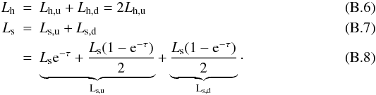 The first equation assumes an isotropic Compton process, and the second equation is obtained with the same reasoning as in Eqs. (B.1) and (B.2).
Then the observed luminosity is simply  (B.9)where we neglect any extra emission that does not come from the corona. From Eqs. (B.6), (B.8), and (B.9), we can deduce Lh
 (B.10)and finally, from Eq. (B.5)
  (B.11)For an optically thin corona (τ ≪ 1), Ltot ≃ 2Lobs − Ls. This is roughly the case for the hot corona. On the other hand, for τ ≫ 1, Ltot ≃ 2Lobs, which corresponds to the case of the warm corona.
The radiative equilibrium of the soft phase (which produces the soft photon field) also implies 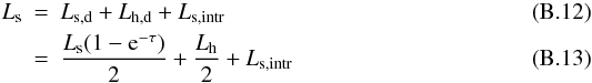 where Ls,intr is the intrinsic emission of the soft phase. In consequence, the heating/cooling ratio is equal to
 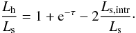 (B.14)In the case of an optically thin (τ < 1) corona above a passive disk (Ls,intr = 0), we found the well known result Lh/Ls = 2 (see e.g. Haardt & Maraschi 1991 and their Eq. (3b) with f = 0 and no disk albedo) and consequently Ltot/Ls = 3. On the other hand, for an optically thick corona (still above a passive disk), we find Lh/Ls = 1 and Ltot/Ls = 2
All Tables
Best-fit parameters of the total spectrum and the different observations using the Comptonization model compps for the primary continuum and nthcomp for the UV-soft X-rays.
All Figures
|
Fig. 1 Count rates light curves in different energy ranges. From top to bottom: 2120 Å, 0.5−1 keV, 3−10 keV, 20−60 keV, and 60−200 keV. The horizontal solid lines are the average values and the horizontal dashed lines represent the corresponding ± 1σ uncertainties. |
| In the text | |
|
Fig. 2 Count rate-count rate correlation coefficients between different energy bands for the 10 observations. In each panel, the green star is the XMM-Newton/OM light curve in the 3−6 eV band; the three blue crosses correspond to the XMM-Newton/pn soft X-ray bands: 0.2−0.5 keV, 0.5−1 keV, 1−2 keV; the three red diamonds correspond to the XMM-Newton/pn medium X-ray bands: 2−4 keV, 4−6 keV, 6−12 keV; and the two black triangles correspond to the INTEGRAL/ISGRI hard X-ray bands: 20−60 keV and 60−200 keV. In each panel, the light curves are correlated with the one marked with the vertical dotted lines. We have overplotted the 95% and 99% confidence levels for the significance of the correlation (it corresponds to correlation coefficients of 0.64 and 0.78, respectively, for 10 points) with horizontal dot-dashed and dashed lines, respectively. |
| In the text | |
|
Fig. 3 First (left panels) and second (right panels) principal components of variability. The upper panels show the spectra corresponding to the maximal and minimal coordinate αj,k over the j = 10 observations of the first (k = 1, left) and second (k = 2, right) eigenvectors. The middle panels show the ratio of the maximum and minimum spectra to the total spectrum of the source. The bottom panels show the contribution of each component to the total variance as a function of energy. |
| In the text | |
|
Fig. 4 Top: total XMM-Newton (pn, black) and INTEGRAL (ISGRI, red) data above 3 keV. The solid line is the best-fit power-law model. Bottom: ratio data/model. The iron line is clearly visible and no high-energy cut-off is required. |
| In the text | |
|
Fig. 5 Unfolded best-fit model of the total data spectrum using a thermal Comptonization component (compps in xspec) for the primary continuum. The data are the black crosses. The solid black line is the best-fit model including all absorption (WA and Galactic). The dashed lines correspond to the different spectral components, hot (in red) and warm (in blue) corona emission as well as the reflection (magenta) produced by pexmon including the effects of absorptions, while the dotted line are absorption free. |
| In the text | |
|
Fig. 6 Contour plots of the temperature versus optical depth for the hot (top) and warm (bottom) corona for the 10 observations. We have overplotted the predicted relationship τ vs. kT in steady state assuming a soft-photon temperature of 10 eV and for different Compton amplification ratios: dotted line: Ltot/Ls = 2; dashed line: Ltot/Ls = 3; dot-dot-dot-dashed: Ltot/Ls = 11. |
| In the text | |
|
Fig. 7 Time evolution of the different fit parameters. From top to bottom: the hot corona temperature kThc, Compton parameter yhc, optical depth τhc, and the warm corona temperature kTwc, photon index Γwc, optical depth τwc, and the soft photon temperatures Tbb,wc and Tbb,hc. The solid lines show the best-fit constant values and the solid lines the ± 1σ uncertainties. |
| In the text | |
|
Fig. 8 a) Total flux Ltot/LEdd emitted by the hot corona and b) intercepted soft photon luminosity Ls/LEdd entering and cooling the hot corona. c) and d), like a) and b) but for the warm corona. e) Compton amplification ratio Ltot/Ls for the warm (bottom curve) and hot (top curve) coronae, respectively. The dotted line in e) is the expected value for a thick corona in radiative equilibrium above a passive disk. All the luminosities are in Eddington units assuming a black-hole mass of 1.4 × 10⁸ M⊙. The error bars on Lobs and Ls have been estimated as on the order of 5%. |
| In the text | |
|
Fig. 9 Correlation of the seed soft-photon luminosity of the hot corona, Ls,hc, and the total luminosity of the warm plasma Ltot,wc. |
| In the text | |
|
Fig. 10 A sketch of the accretion flow geometry in the inner region of the galaxy Mrk 509. The hot corona, producing the hard X-ray emission, has a temperature of ~100 keV and optical depth ~0.5. It is localized in the inner part of the accretion flow (R < Rin) and illuminates the accretion disk beyond Rin, helping to form a warm layer at the disk surface. This warm component has a temperature of ~1 keV and an optical depth ~15 and produces the optical-UV up to soft X-ray emission. It extends over a large part of the accretion flow, heating the deeper layers and comptonizing their optical-UV emission. In return, part of this emission enters and cools the hot corona. |
| In the text | |
|
Fig. 11 Contour plots of the inner disk radius Rin (solid lines, in units of Rg) and the total accretion rate Ṁ (dashed lines, in Eddington units and assuming an accretion efficiency η = (2Risco/Rg)-1) in the Ltot,hc − Ltot,hc/Ltot,wc plane (see Eqs. (1) and (2)). The points indicate the positions of the 10 observations. |
| In the text | |
|
Fig. 12 Hard-to-soft compactness ratio lh/ls vs. hard compactness ls. The figure is extracted from Ghisellini & Haardt (1994). It shows the one-to-one correspondence between the spectral characteristics of the Compton spectrum of a pure pair plasma (energy spectral index α and temperature kT) and the soft and hard compactnesses.The black points correspond to the 10 observations of Mrk 509. |
| In the text | |
|
Fig. 13 Left: lag energy spectrum. It is obtained by computing time lags in Fourier frequency space, between the energy band 0.3 − 10 keV and a number of adjacent energy channels, averaging the resulting lags over the frequency interval 10-5 − 10-4 Hz. Right: coherence between 0.3−1 and 1−10 keV energy bands as a function of Fourier frequency once a correction for the Poisson noise effects is applied (Vaughan & Nowak 1997). |
| In the text | |
|
Fig. A.1 Contours of the temperature (dashed lines) and optical depth (solid lines) in the Γ-kTnth parameter space of nthcomp for compst (top left), comptt (top right) and eqpair (bottom left) respectively. Bottom right: light curves of the optical depth estimates during the whole campaign for the three models: diamonds: compst, squares: eqpair; triangles: comptt. |
| In the text | |
Current usage metrics show cumulative count of Article Views (full-text article views including HTML views, PDF and ePub downloads, according to the available data) and Abstracts Views on Vision4Press platform.
Data correspond to usage on the plateform after 2015. The current usage metrics is available 48-96 hours after online publication and is updated daily on week days.
Initial download of the metrics may take a while.