| Issue |
A&A
Volume 549, January 2013
|
|
|---|---|---|
| Article Number | A72 | |
| Number of page(s) | 13 | |
| Section | Extragalactic astronomy | |
| DOI | https://doi.org/10.1051/0004-6361/201219450 | |
| Published online | 21 December 2012 | |
Multiwavelength campaign on Mrk 509
XI. Reverberation of the Fe Kα line
1 School of Physics and Astronomy, University of Southampton, Highfield, Southampton SO17 1BJ, UK
e-mail: ponti@iasfbo.inaf.it
2 INAF – IASF Bologna, via Gobetti 101, 40129 Bologna, Italy
3 SRON Netherlands Institute for Space Research, Sorbonnelaan 2, 3584 CA Utrecht, The Netherlands
4 Dipartimento di Fisica, Università degli Studi Roma Tre, via della Vasca Navale 84, 00146 Roma, Italy
5 Sterrenkundig Instituut, Universiteit Utrecht, PO Box 80000, 3508 TA Utrecht, The Netherlands
6 Centro de Astrobiología (CSIC-INTA), Dep. de Astrofísica, LAEFF, PO Box 78, 28691 Villanueva de la Cañada, Madrid, Spain
7 UJF-Grenoble 1 / CNRS-INSU, Institut de Planétologie et d’Astrophysique de Grenoble (IPAG) UMR 5274, 38041 Grenoble, France
8 Space Telescope Science Institute, 3700 San Martin Drive, Baltimore, MD 21218, USA
9 Department of Physics and Astronomy, The Johns Hopkins University, Baltimore, MD 21218, USA
10 Instituto de Astronomía, Universidad Católica del Norte, Avenida Angamos 0610, Casilla 1280, Antofagasta, Chile
11 Department of Physics, University of Oxford, Keble Road, Oxford OX1 3RH, UK
12 Department of Physics, Virginia Tech, Blacksburg, VA 24061, USA
13 Department of Physics, Technion-Israel Institute of Technology, 32000 Haifa, Israel
14 Mullard Space Science Laboratory, University College London, Holmbury St. Mary, Dorking, Surrey, RH5 6NT, UK
15 Centrum Astronomiczne im. M. Kopernika, Rabiańska 8, 87-100 Toruń, Poland
16 ISDC Data Centre for Astrophysics, Astronomical Observatory of the University of Geneva, 16 ch. d’Ecogia, 1290 Versoix, Switzerland
17 Department of Astronomy and CRESST, University of Maryland, College Park, MD 20742, USA
18 X-ray Astrophysics Laboratory, NASA/Goddard Space Flight Center, Greenbelt, MD, 20771, USA
Received: 20 April 2012
Accepted: 25 June 2012
Context. We report on a detailed study of the Fe K emission/absorption complex in the nearby, bright Seyfert 1 galaxy Mrk 509. The study is part of an extensive XMM-Newton monitoring consisting of 10 pointings (~60 ks each) about once every 4 days, and includes a reanalysis of previous XMM-Newton and Chandra observations.
Aims. We aim at understanding the origin and location of the Fe K emission and absorption regions.
Methods. We combine the results of time-resolved spectral analysis on both short and long time-scales including model-independent rms spectra.
Results. Mrk 509 shows a clear (EW = 58 ± 4 eV) neutral Fe Kα emission line that can be decomposed into a narrow (σ = 0.027 keV) component (found in the Chandra HETG data) plus a resolved (σ = 0.22 keV) component. We find the first successful measurement of a linear correlation between the intensity of the resolved line component and the 3–10 keV flux variations on time scales of years down to a few days. The Fe Kα reverberates the hard X-ray continuum without any measurable lag, suggesting that the region producing the resolved Fe Kα component is located within a few light days to a week (r ≲ 103rg) from the black hole (BH). The lack of a redshifted wing in the line poses a lower limit of ≥40 rg for its distance from the BH. The Fe Kα could thus be emitted from the inner regions of the BLR, i.e. within the ~80 light days indicated by the Hβ line measurements. In addition to these two neutral Fe Kα components, we confirm the detection of weak (EW ~ 8–20 eV) ionised Fe K emission. This ionised line can be modelled with either a blend of two narrow Fe xxv and Fe xxvi emission lines (possibly produced by scattering from distant material) or with a single relativistic line produced, in an ionised disc, down to a few rg from the BH. In the latter interpretation, the presence of an ionised standard α-disc, down to a few rg, is consistent with the source high Eddington ratio. Finally, we observe a weakening/disappearing of the medium- and high-velocity high-ionisation Fe K wind features found in previous XMM-Newton observations.
Conclusions. This campaign has made the first reverberation measurement of the resolved component of the Fe Kα line possible, from which we can infer a location for the bulk of its emission at a distance of r ~ 40–1000 rg from the BH.
Key words: accretion, accretion disks / black hole physics / methods: data analysis / galaxies: individual: Mrk 509 / galaxies: active / galaxies: Seyfert
© ESO, 2012
1. Introduction
X-ray observations of AGN have shown the almost ubiquitous presence of the Fe Kα line at 6.4 keV (Yaqoob et al. 2004; Nandra et al. 1997, 2007; Bianchi et al. 2007; de la Calle et al. 2010). Unlike the optical-UV lines that are emitted by distant material alone, the Fe Kα line traces reflection not only from distant material (such as the inner wall of the molecular torus, the broad line region and/or the outer disc) but also from regions as close as a few rg (where rg = GM/c2) from the BH (Fabian et al. 2000).
The powerful reverberation mapping technique, which is routinely exploited on optical-UV lines (Clavel et al. 1991; Peterson 1993; Kaspi et al. 2000; Peterson et al. 2004), can also be applied to X-ray lines such as the Fe Kα line. This kind of analysis has tremendous potential, allowing us to map the geometry of matter surrounding the BH, starting from distances of a few gravitational radii up to light years. However, each Fe Kα component is expected to respond on a different characteristic time (years to decades for the torus, several days to months for the BLR-outer disc, and tens of seconds to a few hours for the inner accretion disc), and current X-ray instruments cannot easily disentangle the different components. Indeed, reverberation mapping of all Fe Kα emission components represents an enormous observational challenge, and specially tailored monitoring campaigns (to sample the proper time scales) have to be designed.
Since the detection of the first clear example of a broad and skewed Fe line profile in the spectrum of an AGN (indicating that most of the line emission is produced within a few tens of rg; e.g. MCG-6-30-15, Tanaka et al. 1995), the quest to understand how the broad Fe Kα line varies with the continuum is ongoing. Indeed, close to the BH the simple one-to-one correlation between continuum and reflection line is distorted by General and Special relativistic effects. Several papers present extensive theoretical computations to describe the inner disc reverberation to the continuum by taking all relativistic effects into account (Reynolds et al. 1999; Fabian et al. 2000; Reynolds & Nowak 2003).
Several techniques have been employed to measure the variability-reverberation of the relativistic Fe Kα line. However, for the best cases such as MCG-6-30-15, the relativistic Fe line showed complex behaviour, having a variable intensity at low fluxes (Ponti et al. 2004; Reynolds et al. 2004) while showing a constant intensity at higher fluxes (Vaughan et al. 2003, 2004; see also the case of NG 4051: Ponti et al. 2006). This puzzling and unexpected behaviour has been interpreted by some authors (Miniutti et al. 2003, 2004) as due to strong light bending effects or, alternatively, as evidence that the broad wing of the Fe Kα line is produced by strong and complex absorption effects (Miller et al. 2008).
Thanks to the application of Fe Kα excess emission maps (Iwasawa et al. 2005; Dovciak et al. 2004; De Marco et al. 2009), it has been possible to track weaker coherent patterns of Fe Kα variations. In a few sources Fe Kα variations are consistent with being produced by orbiting spots at a few rg from the BH (Iwasawa et al. 2004; Turner et al. 2006; Petrucci et al. 2007; Tombesi et al. 2007). Future larger area telescopes are needed to finally assess if these features are present only sporadically during peculiar periods or if they, instead, are always present, although weak, and can be used to map the inner disc (see e.g. Vaughan et al. 2008; De Marco et al. 2009).
A leap forward in X-ray reverberation studies occurred thanks to applying pure timing techniques to the long XMM-Newton observation of 1H0707-495 that allowed the discovery of a “reverberation lag” between the direct X-ray continuum and the soft excess, probably dominated by FeL line emission (Fabian et al. 2009; Zoghbi et al. 2010). Soon after, similar delays were seen in a few other objects (Ponti et al. 2010; De Marco 2011; Emmanouloulos et al. 2011; Zoghbi & Fabian 2011; Turner et al. 2011). Recently, De Marco et al. (2012) has shown that these lags are ubiquitous in AGN and that they scale with MBH and have amplitudes close to the light crossing time of a few rg, thus suggesting a reverberation origin of the delay (but see also Miller et al. 2010). Another fundamental step forward will be to combine these timing techniques to detect reverberation lags in the Fe K band (see Zoghbi et al. 2012).
Reverberation from distant material has the advantage that the intensity of the Fe Kα line and the continuum are expected to follow a simple one-to-one correlation, however, the expected delays between the reflection component and the direct emission are usually too large for a typical X-ray exposure. In fact, reflection from the inner walls of a molecular torus is expected to be delayed by a few years up to several decades so it requires a very long monitoring campaign. Reflection from the BLR and/or outer disc is more accessible, the delay between continuum and reflection is expected to be between a few days up to few months. Thus a properly tailored monitoring campaign on a bright AGN with XMM-Newton, Chandra, or Suzaku could achieve this goal. Several attempts have been made (Markowitz et al. 2003; Yaqoob et al. 2005; Liu et al. 2010). However, the 15–20% or larger error on the flux of the Fe Kα line and the low-sampling frequency of the X-ray observations have made applying reverberation of the Fe Kα line on timescales of weeks to months basically impossible, until now.
Mrk 509 (z = 0.034397) is one of the brightest Seyfert 1 galaxies of the (2–100 keV) X-ray sky (Malizia et al. 1999; Revnivtsev et al. 2004; Sazonov et al. 2007), thus it has been observed by all major X-ray/Gamma-ray satellites. The Chandra HETG spectrum shows a narrow component of the Fe K line with an equivalent width (EW) of 50 eV (Yaqoob et al. 2004). XMM-Newton and Suzaku data provide evidence of a second, broader (σ = 0.12 keV) neutral Fe K line (Ponti et al. 2009), as well as of a weak ionised emission feature between 6.7–6.9 keV (Pounds et al. 2001; Page et al. 2003; Ponti et al. 2009). The ionised emission can be fit using either a relativistically broadened ionised line or an outflowing photo-ionised gas component.
Imprinted on the Fe K band emission of Mrk 509 are the fingerprints of two kinds of ionised absorption components, one marginally consistent with a medium velocity outflow (v ~ 14 000 km s-1; Ponti et al. 2009) and the others out(in)flowing with relativistic velocities (Cappi et al. 2009; Dadina et al. 2005; Tombesi et al. 2010).
Here, we present the spectral and variability analysis of the Fe K complex energy band of Mrk 509 using a set of ten XMM-Newton observations (60 ks each, with a cadence of ~4 days and in total spanning more than one month), which were carried out in 2009 (see the 3–10 keV light curve in Fig. 1). We also reanalyse the previous five XMM-Newton observations. Thanks to this extensive monitoring campaign we can measure correlated variations between the Fe K line intensity and X-ray continuum flux, allowing us, for the first time, to perform a reverberation mapping study on this X-ray emission line. In addition we can study the presence of highly ionised matter from the innermost regions around the BH.
The paper is organised as follows. Section 2 is devoted to describing the observations and data reduction. In Sect. 3 a first parametrisation (with a single Gaussian profile for the Fe Kα line) of the total summed spectrum of the 2009 campaign is presented. Section 4 is dedicated to detailed study of the Fe Kα emission. We first present the study of the Fe Kα line variability, assuming a single Gaussian profile (Sect. 4.1) and then use the Chandra HETG data (Sect. 4.2) to decompose the Fe Kα line into two Gaussian (narrow and resolved) components. Section 4.3 presents the correlation between Fe Kα intensity and the 3–10 keV continuum (once the Fe Kα line is fitted with 2 Gaussian lines), which is confirmed, in a model-independent way, by the rms spectrum (Sect. 4.4). In Sect. 4.5 we discuss the possible origin of the Fe Kα line. Section 5 presents the study and discusses the origin of the ionised Fe K emission/absorption. Conclusions are in Sect. 6.
2. Observations and data reduction
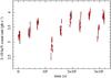 |
Fig. 1 3–10 keV EPIC-pn light curve (3 ks time bins) of the 10 XMM-Newton observations of the 2009 monitoring campaign. |
Mrk 509 was observed for a total of 15 times by XMM-Newton: on 2000–10–25, 2001–04–20, 2005–10–16, 2005–10–20, 2006–04–25, and ten times in 2009 (see Fig. 1 starting from 2009-10-15 and ending on 2009-11-20). Ponti et al. (2009) and Kaastra et al. (2011) provide full descriptions of the first five and the last ten XMM-Newton observations, respectively.
We initially reduced the EPIC data (as in Mehdipour et al. 2011), starting from the ODF files, using the standard SAS v9.0 software. However, we noted that the rest-frame best fit energy of the Fe Kα line in the EPIC-pn spectrum (EFe Kα = 6.35 ± 0.01 keV) was not consistent with the best fit energy in the summed spectrum of the EPIC-MOS data (EFe Kα = 6.41 ± 0.01 keV). This discrepancy (~50 eV) was found to be systematic, and was present in all ten observations. Because it was significantly larger than the reported systematic uncertainty on the calibration of the absolute energy scale of 10 eV (CAL-TN-0018), this result triggered an in-depth study of the pn and MOS energy scales by the XMM-Newton EPIC calibration team. After excluding that this effect is related to X-ray loading, a stronger than expected long-term degradation/evolution of the charge transfer inefficiency (CTI) was found. The pn long-term CTI was thus recalibrated, and its corrected value implemented in the SAS version 10.0.0 (see CCF release note XMM-CCF-REL-2711).
The EPIC data were thus reduced again using the SAS version 10.0.0. During the XMM-Newton monitoring, both the EPIC-pn and the EPIC-MOS cameras were operating in the small window mode with the thin filter applied. The #XMMEA_EP and #XMMEA_EM, for the pn and MOS cameras, respectively, are used to filter the events lists and to create good time intervals (GTI). The FLAG==0 was then used for selection of events for making the spectra. The data were screened for any increased flux of background particles. The contribution from soft protons flares was negligible during the whole 2009 monitoring. The final cleaned EPIC-pn exposures for each XMM-Newton observation were about 60 ks, i.e. roughly 40 ks, after accounting for the proper dead time of the pn when operating in small-window mode (see Table 1 of Mehdipour et al. 2011, for a list of the exposure times).
Best fit results of the summed EPIC-pn spectrum of the 10 XMM-Newton observations performed during the 2009 campaign.
The pn and MOS spectra were extracted from a circular region of 45′′ and 20′′ radius centred on the source, respectively. The background was taken locally from identical circular regions located on the same CCD of the source for the EPIC-pn but on another CCD for the EPIC-MOS. The EPIC data showed no evidence of significant pile-up, thus single and double events were selected for both the pn (PATTERN < = 4) and the MOS (PATTERN < = 12) camera. Response matrices were generated for each source spectrum using the SAS tasks arfgen and rmfgen. The sum of the spectra was performed with the mathpha, addrmf, and addarf tools within the Heasoft package (version 6.10).
Mrk 509 was observed by the Chandra Advanced CCD Imaging Spectrometer (ACIS: Garmire et al. 2003) with the High-Energy Transmission Grating Spectrometer (HETGS: Canizares et al. 2005) in the focal plane, on April 13 2001 (obsid 2087). Data were reduced with the Chandra Interactive Analysis of Observations (CIAO: Fruscione et al. 2006) 4.2 and the Chandra Calibration DataBase (CALDB) 4.3.1 software, adopting standard procedures.
All spectral fits were performed using the Xspec software (version 12.3.0) and include the neutral Galactic absorption (4.44 × 1020 cm-2; Murphy et al. 1996), the energies are in the rest frame if not specified otherwise; however, the energies in the plots are in the observed frame and the errors are reported at the 90 per cent confidence level for one interesting parameter (Avni 1976) in all the tables, while they are 1 σ errors in the figures. Mrk 509 has a cosmological redshift of 0.034397 (Huchra et al. 1993) corresponding to a luminosity distance of 145 Mpc (taking ⟨ H0 ⟩ = 73 km s-1 Mpc-1, ΩΛ = 0.73, and Ωm = 0.27).
3. The mean spectrum
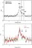 |
Fig. 2 Upper panel: summed EPIC-pn spectra of the 10 observations performed during the 2009 XMM-Newton monitoring campaign. The data are fit, in the 4–5 and 7.5–10 keV bands, with a simple power law, absorbed by Galactic material, and the ratio of the data to the best-fit model is shown. The dotted lines indicate the rest frame positions of the Fe Kα, Fe Kβ, Fe xxv (resonance, intercombination and forbidden), and Fe xxvi lines. The x-axis reports the observed-frame energy. Lower panel: in red the 2006 XIS0+XIS3 Suzaku summed mean spectra are shown. In black the summed spectra of the 5 XMM-Newton observations performed between 2000 and 2006 are shown. This figure is taken from Ponti et al. (2009). The arrows mark possible absorption features in the spectrum. |
The upper panel of Fig. 2 shows the data to best fit model ratio plot of the summed spectra of the ten EPIC-pn observations performed during the 2009 XMM-Newton monitoring campaign, fitted in the 3.5–5 and 7.5–10 keV band with a simple power law, which was absorbed by Galactic material (interstellar neutral gas; phabs model in Xspec). For comparison, the black data points in the lower panel of Fig. 2 show the same plot for the summed EPIC-pn spectrum of the previous five XMM-Newton observations taken between 2000 and 2006, while the red data show the summed XIS0+XIS3 spectra of the four Suzaku observations performed between April and November 2006 (see Ponti et al. 2009, for more details).
Thanks to a longer integrated exposure and a slightly higher flux, the source spectrum in the Fe K band has significantly better statistics during the 2009 campaign than the sum of all the previous observations (see Fig. 2). We can thus constrain the Fe K complex better and study its variability not only on the time scales of days and weeks over which the monitoring has been performed, but also on time scales of years, using previous observations.
The upper panel of Fig. 2 shows an evident emission line at 6.4 keV, as well as an emission tail at higher energies, as observed during previous observations. A simple power law fit to the 4–10 keV total pn spectrum gives an unacceptable fit (χ2 = 2445.7 for 1197 d.o.f.). Adding a Gaussian line to fit the Fe Kα line at 6.4 keV improves the fit by Δχ2 = 1134 for three extra parameters (see model 1 in Table 1). This line reproduces the bulk of the neutral Fe K emission (E = 6.43 ± 0.01 keV), but leaves strong residuals at higher energies, which might be, at least in part, associated with an Fe Kβ emission line. We thus add a second line with the same line width as the Fe Kα line and an energy of 7.06 keV (Kaastra & Mewe 1993). The best fit parameters are given as model 2 in Table 1, and the fit improves by Δχ2 = 66.9 for the addition of one new parameter. The best fit intensity is NFe Kβ = 0.75 × 10⁻⁵ ph cm-2 s-1, and the observed Kβ/Kα ratio is =0.19 ± 0.02. This is slightly, but significantly, higher than 0.155–0.16, the value estimated by Molendi et al. (2003; who assume the Basko 1978 formulae; but see also Palmeri et al. 2003a,b). The excess of Fe Kβ emission might be due to the contamination by the Fe xxvi emission line at 6.966 keV. This idea is further supported by the observation of clear residuals, in the best fit, around 6.7 keV; and by the best fit Fe K energy (E = 6.43 ± 0.01 keV), which is inconsistent with the line arising from neutral iron. This thus suggests that the Gaussian line is trying to fit both the neutral and ionised Fe K components.
To model ionised Fe K emission, we add two narrow (σ = 0) emission lines, one (Fe xxv) emitting between 6.637 and 6.7 keV (to take emission for each component of the triplet into account) and the other (Fe xxvi) emitting at 6.966 keV (model 3 in Table 1). Moreover, we require that the intensity of the Kβ has to be 0.155–0.16 times the intensity of Fe Kα one (and σFe Kβ = σFe Kα). The fit significantly improves (Δχ2 = 25 for the addition of one more parameter). Both Fe xxv (the best fit line energy is consistent with each one of the triplet) and Fe xxvi are statistically required (although the Fe xxvi line is not resolved from the Fe Kβ emission, so its intensity depends on the assumed Kα/Kβ ratio). In this model the Fe Kα line is roughly consistent with being produced by neutral or low ionisation material (EFe Kα = 6.415 ± 0.012 keV).
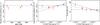 |
Fig. 3 (Left, middle and right panels) Intensity vs. time in MJD, intensity vs. 3–10 keV flux and EW vs. 3–10 keV flux of the Fe Kα line fitted with a single Gaussian profile with σ = 0.092 keV (model 1), respectively. Each data point represents the best fit result obtained from the fit of the spectrum of each XMM-Newton observation (red hexagonals) and the total spectrum of the 2009 data (blue stars). The dashed lines represent the expected relations if the Fe Kα line has constant intensity, while the dash-dotted lines represent a constant EW, and the dotted line shows the best fit trend. The left panel show the observation date in Modified Julian Date, MJD minus 51 500, which corresponds to November 18, 1999. Two XMM-Newton observations occur at day 2159 and day 2163 and appear to overlap in the left panel. |
Pounds et al. (2001), Ponti et al. (2009), de la Calle et al. (2010), Cerruti et al. (2011), and Noda et al. (2011) suggest that the inner accretion disc in Mrk 509 might be highly ionised, and thus the ionised emission of the Fe K complex might be associated to a relativistic ionised reflection component produced in the inner disc. To test this hypothesis, we substitute the two narrow lines (Fe xxv and Fe xxvi) with one broad ionised line (model 4 in Table 1) with a relativistic profile (disc line profile for a Schwarzschild black hole; diskline model in Xspec). We fixed the line energy either to 6.7 or 6.96 keV (for the Fe xxv or Fe xxvi lines, respectively) and the inner and outer disc radius to 6 and 1000 gravitational radii. In both cases the best fit with this model suggests that the inner accretion disc to be moderately inclined ~33–18°, to have a fairly standard disc emissivity index − 2.2 − 2.8 and an EW of the line of EW ~ 36–40 eV. The data are described reasonably well by this model, resulting in a χ2 = 1216.0 for the case of a broad Fe xxv and χ2 = 1219.4 for 1191 d.o.f. for Fe xxvi line. Thus, the single broad ionised disc-line model is statistically indistinguishable from the multiple narrow lines one (χ2 = 1219.8 for 1192 d.o.f.).
3.1. Medium velocity-high ionisation winds
The summed spectrum of the previous XMM-Newton observations showed a medium velocity (vout ~ 0.048 ± 0.013 c), highly ionised (Log(ξ) ~ 5) outflow in Mrk 509 (Ponti et al. 2009). The associated Fe xxvi absorption line was detected both in the EPIC-pn and the MOS camera, with  eV and with a total significance between 3–4σ (~99.9% probability).
During the 2009 XMM-Newton campaign this highly ionised absorption component is not significantly detected. If we add a narrow Gaussian absorption line at 7.3 keV, the energy of the absorption feature in the previous XMM-Newton observations, we observe the line to be much weaker with the best fit line EW being  eV, significantly smaller than observed in previous XMM-Newton observations.
4. The neutral Fe Kα component
In this section we investigate the nature of the Fe Kα line further, looking at the individual spectra obtained over the years. Our analysis of the long 2009 monitoring campaign, which triples the total exposure on Mrk 509, confirms there is a resolved component (σ = 0.092 ± 0.012 keV) of the neutral Fe Kα line (see model 3, but also 4 and 5 of Table 1).
4.1. Fe Kα variations on timescales or years
To study the variability of the neutral Fe Kα emission line (on time scales of years), we fit the spectrum of each of the old XMM-Newton observations (i.e. between 2000 and 2006) with a single Fe Kα (plus associated Kβ emission) plus two narrow emission lines (such as in Sect. 3 in model 3) to parametrise the ionised Fe K emission (see Table 1). Leaving the Fe Kα widths free to vary, as in Table 1, would result in unconstrained values for the spectra with the shortest exposures (due to the lower statistics). We thus decide to fix the width of the Fe Kα line to σ = 0.092 keV, its best fit value as observed in the total spectrum of the 2009 campaign (model 3 of Table 1).
The left-hand panel of Fig. 3 shows the Fe Kα line intensity for each XMM-Newton observation as a function of time, using the summed 2009 data. The line intensity is observed to vary by less than 25%. The fit with a constant Fe Kα intensity (dashed line), however, is unsatisfactory (χ2 = 10.7 for 5 d.o.f.). The middle panel of Fig. 3 shows the Fe Kα intensity vs. source flux in the 3–10 keV band. The fit slightly improves when a linear relation (see dotted line) is considered (Δχ2 = 7.6 for the addition of one more parameter; 97% F-test probability). The increase in Fe Kα intensity with flux might suggest that the line is responding quickly to the illuminating continuum, keeping a constant EW with flux. The dash-dotted line shows the expected Fe Kα intensity variation for a line with constant EW. The observed line intensity variations are intermediate between the constant intensity and constant EW cases. The right-hand panel of Fig. 3 confirms that the line has neither constant intensity nor constant EW; instead it sits somewhere in the middle between these two cases.
Best fit results of the summed EPIC-pn spectrum of the 10 XMM-Newton observations performed during the 2009 campaign and of the XMM-Newton observations performed between 2000 and 2006.
Best fit results of the summed EPIC-pn spectrum of the 10 XMM-Newton observations performed during the 2009 campaign.
The Fe Kα variations on time scales of years suggest that at least part of the line is varying following the 3–10 keV continuum. We want to point out that the width of the Fe Kα line is comparable to the EPIC-pn energy resolution. This means that the observed Fe Kα variability may be the product of a constant narrow component, coming from distant material, plus a broader, resolved, and variable Fe Kα line produced closer to the BH. Unfortunately, due to the limited energy resolution of the EPIC cameras aboard XMM-Newton, we cannot resolve the Fe K emission, coming from regions located light weeks from those at light years from the BH, based on the Fe Kα line widths. Only with the Chandra high-energy transmission grating (HETG) we can confidently place some constraints on the distance of the different Fe K emission components.
4.2. Chandra HETG
Chandra observed Mrk 509 with the HETG instrument only once for 50 ks (Yaqoob et al. 2003). During the HETG observation the 3–10 keV flux was 4.36 × 10⁻¹¹ erg cm-2 s-1 with a power law spectrum of index  . An excess was present at 6.4 keV, so we added a Gaussian line2. In agreement with the results obtained by Shu et al. (2010) and Yaqoob & Padmanabhan (2004), we detect a line at 6.42 ± 0.02 keV with an intensity of 3 ± 2 × 10⁻⁵ photons cm-2 s-1. The line is resolved and has a significantly smaller width than the one measured by XMM-Newton,
  keV. This suggests that at least part of the neutral Fe Kα emission is produced in regions more distant than a few thousand gravitational radii. In fact, if the material is in Keplerian motion and assuming a BH mass of Mrk 509 of MBH = 1.4 − 3 × 10⁸M⊙ (Peterson et al. 2004; Mehdipour et al. 2011), then the narrow core of the line is produced at a distance of r = 0.2–0.5 pc (~30 000 rg). We note that this value is within an order of magnitude of the molecular sublimation radius for Mrk 509. Landt et al. (2011) uses quasi-simultaneous near-infrared and optical spectroscopy to estimate a radius of the hot dust of ~0.27 pc (0.84 ly), which is also consistent with the one estimated following Eq. (5) of Barvainis (1987) assuming a bolometric luminosity LBol = 1.07 × 1045 erg s-1 (Woo & Urry 2002). This suggests that this narrow component of the Fe K line might be associated to the inner wall of the molecular torus.
4.3. Two components of the Fe Kα line
Thus, as suggested by the analysis of the Chandra HETG data and in agreement with the observed variability on time scales of years, we interpret the Fe Kα line as being composed of two components that are indistinguishable at the EPIC resolution. We first refit the mean spectrum of the 2009 campaign with two components for the Fe Kα line. The model contains one “narrow” component with the line width fixed at the best fit value derived from Chandra analysis (σ = 0.027 keV) plus a “resolved” component with its width free to vary. Model 6 in Table 2 shows the best fit results when assuming the energy of both components is the same. The narrow component has a best fit EW = 27 ± 4 eV, while the resolved neutral line has an  eV and a best fit line width σ = 0.22 ± 0.05 keV, which is larger than the single Gaussian Fe Kα fit (σ = 0.092 keV).
Reflection is the most probable origin of the Fe Kα line. Associated to reflection lines, an underlying reflection continuum is expected and generally observed. In particular the ratio between the intensity of the line over the reflection continuum strongly depends on the reflector column density reaching a value of EWFe Kα ~ 1 keV for Compton thick materials. To check the impact of the reflection continuum on the best fit model, we added a standard neutral reflection continuum (pexrav in Xspec) with intensity such that the EWFe Kα = 1 keV over their reflection continua. The new best fit line EWs do not vary significantly (EW = 26 ± 3 eV and  eV, for the narrow and resolved Fe Kα lines, respectively). Thus, and considering also the limited energy band used here we decided to disregard the continuum reflection component. The impact of the reflection component on the broad band source emission will be studied by Petrucci et al. (2012) taking the UV to soft gamma ray emission with physical models into account. The narrow component, as observed during the 2009 campaign, has an intensity of 1.5 ± 0.2 × 10⁻⁵ ph cm-2 s-1, which is about half the total Fe Kα intensity (see Table 1 and Fig. 3). This value is consistent with the intensity of the narrow Fe Kα line observed by Chandra. The width of the narrow component suggests a distance of 0.2–0.5 pc from the BH, thus we expect that all the variability on time scales shorter than a few years would be smeared out because of light travelling effects. For this reason and because the lower signal-to-noise in the individual 2009 and earlier XMM-Newton spectra does not allow us to disentangle both components, we assume a constant intensity of 1.5 × 10⁻⁵ cm-2 s-1 for this narrow Fe Kα component in all the following fits.
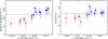 |
Fig. 4 (Left and right panels) The intensity and EW of the resolved (σ = 0.22 keV) Fe Kα component (the narrow Fe Kα component is assumed to have σ = 0.027 keV and be constant) as a function of the 3–10 keV flux. Blue stars and red hexagonals show the best fit results of the 10 observations of the 2009 campaign and of the previous XMM-Newton observations, respectively. Dashed and dot dashed lines show the constant intensity and constant EW cases, respectively. The best fit relation (dotted line) is consistent with the resolved component of the Fe Kα line having constant EW. The intensity of the resolved component of the Fe Kα line follows the 3–10 keV continuum variations with a 1-to-1 relation. |
Next, we fit the spectrum of each of the 15 XMM-Newton observations with model 6, as shown in Table 2, assuming a constant intensity for the narrow Fe Kα component and constant width for the resolved component, plus the associated Fe Kβ and narrow Fe xxv and Fe xxvi lines. The left-hand panel of Fig. 4 shows the intensity of the resolved component (σ = 0.22 keV) vs. the 3–10 keV flux for the ten observations of the 2009 monitoring (blue stars) as well as for the previous XMM-Newton observations (red hexagonals). The dashed line shows the best fit assuming that the Fe Kα intensity is constant, which results in an unsatisfactory fit with χ2 = 33.2 for 14 d.o.f.. On the other hand, once the data are fitted with a linear relation (dotted line), the fit significantly improves (Δχ2 = 23.0 for the addition of one new parameter, which corresponds to F-test probability >99.98%). We also compute that the Pearson’s linear correlation coefficient is equal to 0.87 and has a probability =2.7 × 10⁻⁵, which corresponds to a significance of the correlation of more than 4σ (similar results are obtained using a Spearman’s rho or Kendall’s tau correlation coefficients). The slope of the observed best fit relation is consistent with what is expected if the resolved line is responding linearly to the continuum variations. This is confirmed in the right-hand panel of Fig. 4, which shows that the resolved Fe Kα line EW is consistent with being constant (χ2 = 17.1 for 14 d.o.f.), as expected if the Fe Kα line is responding linearly to the 3–10 keV continuum flux variations.
The line intensity is significantly variable even on time scales of a few days, e.g. between the different pointings of the 2009 monitoring campaign. In fact, fitting the 2009 Fe Kα intensities with a constant gives a χ2 = 13.7 for 9 d.o.f., which becomes χ2 = 5.3 when a linear relation is considered (as specified in Sect. 2, conservative 90% errors are used here). The Pearson’s linear correlation coefficient turns out to be 0.8 and has a probability =5 × 10⁻³, which corresponds to a significance of the correlation of about 3σ.
Figure 5 shows the variations in the intensity of the resolved component of the Fe Kα line as a function of time (1σ errors are shown here), during the 2009 campaign, overplotted on the 3 − 10 keV rescaled flux (dashed line). As already suggested above and in Fig. 4, the Fe K line variations track the continuum very well. We also note that no measurable lag is present, thus this broad component of the Fe Kα line responds to the X-ray continuum within less than four days.
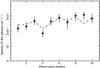 |
Fig. 5 Intensity vs. observation number of the 10 XMM-Newton pointings of the 2009 campaign. The black dashed line shows the rescaled (with the mean 3–10 keV flux equalling the mean line intensity) 3 − 10 keV source flux. The intensity of the resolved component of the Fe Kα line follows, with a 1-to-1 relation the 3–10 keV continuum variations without any measurable lag. 1σ errors are shown. |
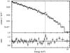 |
Fig. 6 Long time scales, total rms spectrum between the different observations. The spectrum is calculated with time bins of 60 ks (corresponding to the exposure of each XMM-Newton pointing) and the total monitoring time of about 1 month. An excess of variability is clearly evident at 6.4 keV (EW = 71 ± 36 eV). This excess confirms the correlated variability of the resolved Fe K line component in a model independent way (see Fig. 5). |
4.4. Total RMS spectra
Figure 6 shows the total root mean square variability (rms) spectrum calculated between the ten different observations of the 2009 campaign. The rms has been calculated with ten time bins, each one being a 60 ks XMM-Newton pointing. Thus this rms is sampling the variability within the observation separation time scale of about four days and the monitoring time scale of slightly more than one month (see Fig. 1). The total rms shows the spectrum of the variable component, only. Thus, in contrast to the mean spectrum, it has no contribution from the constant emission from distant material (i.e. the narrow core of the Fe K line). The uncertainties on the total rms are derived from the uncertainties on the fractional variability (see formula B.2 of Vaughan et al. 2003; A.1 of Ponti et al. 2004) multiplying for the mean and taking its error into account.
The 3–10 keV total rms spectrum has a power-law shape with spectral index Γ = 1.98 ± 0.06 and normalisation of 1.05 ± 0.05 × 10⁻³ ph cm-2 s-1 (see Fig. 6). A clear excess of variability is present at 6.4 keV. The addition of a Gaussian line significantly improves the fit (Δχ2 = 10.6 for the addition of 2 d.o.f., which corresponds to an F-test significance of 99.3%). The best fit energy of the line is E = 6.45 ± 0.08 keV and intensity (2 ± 1) × 10-6 ph cm-2 s-1. The width of the line is constrained to be less than ~0.2 keV, consistent with the variable, resolved neutral Fe K line. The equivalent width in the total rms spectrum is EW = 71 ± 36 eV, consistent with the EW of the resolved component observed in the mean spectrum. The detection of this excess of variability indicates, in a model-independent way, that the resolved component of the line is varying linearly with the continuum on these time scales. This reinforces the robustness of the detection of Fe K reverberation.
4.5. Locating the Fe Kα emitting region
Do the observed variability properties agree with the spectral ones? Assuming that the material producing the resolved Fe K line is in Keplerian motion around the BH, the line width (σ = 0.22 keV) implies that it is located at 300–1000 rg from the BH. Assuming a BH mass of Mrk 509 of MBH = 1.4 − 3 × 10⁸M⊙ (Peterson et al. 2004; Mehdipour et al. 2011), then this distance corresponds to about a few light days to a light week. The typical spacing between the different XMM-Newton observations during the 2009 monitoring is about four days, thus it is in very good agreement with the observed Fe Kα variations. Moreover, the fast response of the Fe Kα flux to the continuum changes indicates that the bulk of the resolved Fe Kα emission is produced around or within several hundred up to a few thousand gravitational radii from the central BH.
It is more difficult, however, to pose a lower limit to the position of the Fe Kα emitting region. We note that if the Fe Kα line emitting region extends down to a few gravitational radii from the BH, then the line shape should present a prominent red wing. Thus, we fit the resolved component of the Fe Kα line with a disc line profile (diskline in Xspec). In the fitting process we allow the line energy to vary in the range 6.4–6.42 keV. Then we fix the disc outer radius to 1000 rg and the illumination profile to α = −3 (the expected value for a standard alpha disc; Laor 1991; Wilkins & Fabian 2011). The lack of relativistic redshifted Fe Kα emission suggests an inner radius larger than ~85, 45, and 37 rg (which corresponds to roughly 8–16 light hours) for a disc inclination of 30, 20, and 10 degrees, respectively. Thus, the resolved component of the Fe Kα line is probably emitted between 40–1000 rg from the BH.
Can such a “narrow” disc annulus produce an Fe Kα line of ~40–50 eV? Reflection from an accretion disc with solar iron abundances covering half of the sky is expected to produce an Fe Kα line with EW ~ 100–150 eV (Matt et al. 1991). The line EW is expected to decrease/increase roughly linearly/logarithmically for iron abundances lower/higher than solar (Matt et al. 1996, 1997). Steenbrugge et al. (2011) measured a relative iron to oxygen abundance of Fe/O = 0.85 ± 0.06 in Mrk 509. Assuming that this translates into an iron abundance of 0.85 solar (but see Arav et al. 2007), this would correspond to EWFe Kα ~ 90–130 eV. If the primary X-ray source in Mrk 509 is compact (as the variability suggests; McHardy et al. 2006; Ponti et al. 2012b) and located at a few rg above the BH. If the disc is flat, we can estimate (neglecting relativistic effects) the geometric solid angle covered by the disc annulus producing the Fe Kα line (rin ~ 40 and rout ~ 1000 rg) and if the primary X-ray source is located between 1 rg and 4 rg above the BH (De Marco et al. 2012), the flat disc annulus covering factor would be between 2% and 5% of the sky. Thus reflection from such a flat annulus would produce (even in the extreme case of a Fe Kα EW = 130 eV for a standard disc) a line with EW ~ 4–13 eV. The observed EW of the resolved and variable Fe Kα line is several times larger (EW = 42 eV) than this estimated value. This indicates a larger covering factor of the reflector, compared to the flat disc, suggesting that the material producing the Fe Kα line is distributed azimuthally above the disc, possibly in the form of clouds, perhaps associated to the inner BLR (see Costantini et al. 2012, for more details).
The observed correlation on time scales of days to weeks also constraints in which part of the BLR the Fe Kα line is produced. We can exclude, in fact, that the Fe Kα emission is produced in the optical BLR (producing the bulk of Hβ emission), because the Hβ line is observed to reverberate with a delay of 80 days, hence significantly more distant than the region producing the Fe Kα line. On the other hand, several studies show that the BLR might be stratified, with the higher ionisation lines located closer to the central BH. The correspondence between Fe Kα and the inner BLR is reinforced by the consistency between the width of the Fe Kα line (σ = 0.21 ± 0.07 keV, which corresponds to FWHM ~ 1.5−3 × 10⁴ km s-1) and the ones of the broadest components of the UV broad emission lines (e.g. Lyα, C iv, C iii and O vi) which have components with FWHM ~ 104 km s-1 (Kriss et al. 2011).
The lack of relativistic effects on the shape of the Fe Kα line suggests the absence of a neutral standard thin accretion disc extending down to a few gravitational radii from the BH. However, this appears to be at odds with the high efficiency (LBol ~ 5–10% LEdd) of the disc emission of Mrk 509 (Mehdipour et al. 2011; Petrucci et al. 2012). This leads to the question of why we do not find traces of the inner accretion disc in the Fe Kα line shape if it is present in this source.
5. The ionised Fe K emission
During both the 2009 campaign and the previous XMM-Newton observations, Mrk 509 clearly showed an excess of emission around 6.7–7 keV (see Fig. 2) most probably associated to emission from ionised iron. As shown in Sect. 3 this excess can be modelled both by the combination of narrow emission lines from Fe xxv and Fe xxvi, or by a single relativistic emission line (see Table 1). The parameters of this weak ionised emission line(s) can be affected by modelling the stronger Fe Kα line. For this reason, we now refit the mean spectrum including both the narrow and the resolved component of the Fe Kα line.
We first consider that the ionised emission is produced by narrow emission lines (Fe xxv and Fe xxvi). Such emission lines from highly ionised ions are now observed often (Costantini et al. 2010; e.g. for a compilation of sources, Bianchi et al. 2009a,b; Fukazawa et al. 2011), and they can arise from photo-ionised (Bianchi et al. 2005; Bianchi & Matt 2002) or collisionally ionised plasma (Cappi et al. 1999). Thus we fit the spectrum with two components for the Fe Kα line and the associated Kβ lines, plus two narrow (σ = 1 eV) Gaussian emission lines, one (Fe xxv) with energy constrained to be between 6.637 and 6.7 keV, and the other (Fe xxvi) with energy fixed at E = 6.966 keV (see model 6 in Table 2). The model reproduces the data well (χ2 = 1198.5 for 1190 d.o.f.). The weakness of the Fe xxv and Fe xxvi lines prevents us from significantly constraining the line variability between the different XMM-Newton observations.
For comparison, we fit the same model also to the summed spectrum of all XMM-Newton observations taken between 2000 and 2006 (see model 7 of Table 2). The ionised emission lines are consistent with being constant within the two sets of observations. However, the statistics are not good enough to tell whether it is the line intensity (which would suggest an origin at large distances) or the EWs that remain constant. Clear is, instead, the variation in the medium outflow velocity’s highly ionised absorption line, which almost disappeared during the 2009 campaign. The addition of this component to the model used to fit the combined spectra of the 2009 campaign, improves the fit by Δχ2 = 4.5 for two new parameters, which corresponds to an F-test probability of ~90%. Thus we decided to disregard this absorption component in all subsequent fits.
Another clear difference compared to previous observations is related to the disappearance of the highly ionised absorption with mildly relativistic (up to 0.14–0.2c) outflow velocities (Dadina et al. 2005; Cappi et al. 2009; Tombesi et al. 2010). We searched, in fact, for such features in all ten observations obtained after the XMM-Newton campaign, by including narrow absorption lines in the model between 4–10 keV. We found only a marginal (Δχ2 ~ 6) detection of two absorption features at 9 keV and 10.2 keV (rest-frame energies) during observation 4. Even if consistent with being produced by Fe xxvi Kα and Kβ at v ~ 0.3c, and similar to earlier results (Cappi et al. 2009), the level of (highly) ionised absorption during the XMM-Newton campaign is found to be significantly reduced compared with most previous XMM-Newton observations. We obtained upper limits (at 90% confidence) on the equivalent width of narrow (σ fixed to 100 eV) Gaussian absorption lines with typical values between –5 and –30 eV, between 7.5 and 9.0 keV, depending on the energy and observation considered. This is typically lower than values (between –20 and –30 eV) found in the lines detected in earlier observations (Cappi et al. 2009; Tombesi et al. 2010) excluding that such UFOs were present during the 2009 campaign.
5.1. Collisionally ionised plasma
We attempt to interpret the highly ionised emission lines via a self-consistent physical model. First we applied the collisionally ionised model CIE3 in spex (Kaastra et al. 1996). In this fit we considered the 3.5–10 keV band for the continuum. We used Gaussian components for the Fe Kα line profile and Fe Kβ, constraining the flux of the latter to be 0.155–0.16 times the Fe Kα one (Palmeri et al. 2003). This was done in order to mitigate the degeneracy induced by the partial blend with the Fe xxvi Ly α line. The best fit points to a high-temperature gas (kT = 8.5 ± 1.5 keV). At this temperature, the predicted line fluxes are ~5 × 10⁻⁶ ph cm-2 s-1 and ~3 × 10⁻⁶ ph cm-2 s-1 for the Fe xxv triplet and the Fe xxvi Ly α, respectively. These values are consistent with those measured empirically using Gaussian lines (i.e. Table 2). In theory these lines may be produced by hot, line-emitting gas in the form of a starburst driven wind. Mrk 509 has a total luminosity L2 − 10 keV = 1.3 × 1044 erg s-1 in the 2–10 keV band. Assuming an Fe abundance of 0.4 solar (as observed in starburst galaxies, Cappi et al. 1999), the best fit thermal starburst model requires a luminosity L2 − 10 keV = 3.3 × 1042 erg s-1 to reproduce the Fe xxv and Fe xxvi line emission (reducing to L2 − 10 keV = 1.6 × 1042 erg s-1 for solar iron abundance). Using the correlation between L2 − 10 keV and the far infrared luminosity (LFIR), valid in star forming galaxies (Ranalli et al. 2003), we estimate a corresponding LFIR > 1046 erg s-1 and a star-formation rate higher than 400 M⊙ yr-1, which is several times higher than the actual total IR luminosity of Mrk 509, LIR ~ 2 × 10¹¹ L⊙ ~ 8 × 1044 erg s-1 (Rieke et al. 1978), thus we do not favour this interpretation.
5.2. Photo-ionised plasma
Alternatively, the highly ionised lines may be produced by a photoionised plasma. To test this we used a grid of parameters created using Cloudy (Ferland et al. 1998) where the column density logNH of the gas ranged between 21.7−24.5 cm-2 and the ionisation parameter log(ξ) ranged between 3.4 and 7. The grid has been calculated using a covering factor of one. Since the intrinsic line luminosity scales linearly with the covering factor, we used the ratio between the model and the data of the Fe xxvi line as a reference for the covering factor. In Mrk 509, only Fe xxvi and Fe xxv have significant detections, while we have obtained upper limits from the RGS spectrum for other narrow lines from highly ionised ions (e.g. O viii at 18.97 Å and Ne X at 12.13 Å). These limits are useful in constraining the model (i.e. Costantini et al. 2010). In Fig. 7 we compare the line luminosities observed with those computed for a range of models that can fit the data. To reproduce the luminosity of the highly ionised iron ions, the gas should have log(ξ) = 4−5.1 and NH = 23.4−24.2. The covering factor is CV = 0.3−0.5. As we do not see any associated absorption, the gas must be out of the line of sight. Such lines might possibly originate in e.g. the narrow line region or the highly ionised skin of the torus (Bianchi et al. 2005; Bianchi & Matt 2002).
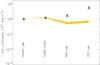 |
Fig. 7 Photoionisation modelling for the highly ionised iron ions Fe xxvi and Fe xxv. Triangles: data. Light shaded line: range of models viable to fit the data. |
5.3. Ionised reflection from inner disc
As shown in Sect. 3, the ionised emission can be fitted equally well with an ionised relativistic emission line. A comparably good fit is also obtained with a broad Gaussian Fe xxv profile in addition to the double Fe Kα + β lines. We fix the energy of the broad Fe xxv line to E = 6.7 keV. The line is significantly broadened σ = 0.23 keV and moderately intense (EW = 15 eV). Although this broadening is not as extreme as to exclude a simple Compton broadening on the ionised surface of the accretion disc, we decided to fit the ionised emission with a relativistic disc line profile, as an alternative to the Gaussian line. An acceptable fit is also obtained in this case (χ2 = 1204.7 for 1192 d.o.f.). Assuming a standard disc emissivity index, inclination, and outer disc radius of β = −3, α = 30° and rout = 200 rg, the best fit disc inner radius is rin = 27 rg, consistent with a value as small as rin = 7 rg, and the disc-line equivalent width is  eV.
eV.
It is difficult to estimate the line EW expected from an ionised inner annulus of the disc. In fact the Fe xxv and Fe xxvi line EW strongly depend on the poorly constrained disc ionisation parameter (Garcia et al. 2011) and on the disc annulus covering angle. However, for reasonable values of these parameters (annulus covering angle ~ 20–40% of the sky and log(ξ) ~ 2.8 − 3.5 erg cm-2 s-1, which corresponds to the peak of Fe xxv and Fe xxvi emission), the line EW is expected to be between 5–50 eV. These results suggest that the inner part of the accretion disc might be highly ionised, thus explaining the lack of detection of relativistic Fe Kα line, combined with the high source efficiency (which suggests a thin standard accretion disc extending all the way down to the last stable orbit).
6. Discussion and conclusions
We investigated the spectral variability of the Fe K band in the nearby, bright Seyfert 1 galaxy Mrk 509, using the ten observations of the 2009 XMM-Newton monitoring campaign, as well as all the previous XMM-Newton observations, with the total exposure more than 900 ks in about ten years, resulting in one of the best quality Fe K spectra ever taken of a Seyfert 1 galaxy. This allows us, for the first time, to perform reverberation mapping of the resolved Fe Kα line.
Figure 8 sketches a possible scenario for the production of the Fe K emission in Mrk 509. The width of the narrow core of the Fe Kα line suggests an origin from distant material, possibly the inner wall of the molecular torus located at 0.2-few pc. The correlated variations (on a few days time scales) between the 3 − 10 keV continuum and the intensity of the resolved component of the Fe Kα suggest an origin between several tens and a few thousand rg from the BH. The resolved Fe Kα emission can be produced in the disc, but we favour an origin at the base of a stratified broad line region. We note that none of the X-ray or UV absorption components with measured location is co-spatial with the resolved Fe Kα emitting region. Moreover, the properties of the X-ray and UV absorbers appear to differ from the ones required to produce the resolved Fe Kα line, suggesting that this emitting material is outside the line of sight, possibly in the form of an equatorial disc wind such as is observed in stellar mass black holes in the soft state (Ponti et al. 2012b) and neutron stars (Diaz-Trigo et al. 2006). The ionised Fe K emission might be produced either by photo-ionisation from distant material, such as the narrow line region and/or the ionised skin of the torus, or in the ionised inner accretion disc.
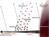 |
Fig. 8 Sketch of possible locations for the different regions producing Fe K emission (diagram not to scale). The star represents the primary X-ray source, located close to the BH. |
The results of this study show that:
-
The XMM-Newton spectrum of Mrk 509 shows an evident Fe Kα line with total EW = 58 ± 4 eV. Fitted with a single Gaussian line the width is σ = 0.092 ± 0.012 keV. The line intensity increases with the 3–10 keV flux, but not as strongly as expected in a constant EW scenario, suggesting the presence of a constant and a variable Fe Kα line component.
-
The Chandra HETG spectrum has enough energy resolution to resolve the narrow component of the Fe Kα line (
keV; line intensity (1.5 ± 0.2) × 10-5 ph cm-2 s-1). The width of the narrow component of the line suggests an origin at around 0.2–0.5 pc (~30 000 rg) from the BH. This value is within an order of magnitude of the molecular sublimation radius, suggesting that the narrow component of the Fe Kα line might be produced as reflection from the inner walls of the molecular torus. If so, because of light travelling effects, the intensity of this component has to be constant on time scales of years. We assume the presence of a constant narrow Fe Kα line (as observed by Chandra HETG) and add a second, resolved (now observed to be broader σ = 0.22 ± 0.04 keV), Fe Kα component with eV. There is excess emission at 7.06 keV, consistent with being produced (at least in part) by the associated Fe Kβ emission. -
For the first time, reverberation mapping of the resolved component of the Fe Kα line on timescales of several days to years was successfully performed. The intensity of the resolved Fe Kα component shows a significant (~4σ) one-to-one correlation with the 3–10 keV flux variability; however, the EW stays constant during the nine years XMM-Newton observed the source. The robustness of this result is confirmed by the results of the rms spectra that, in a model independent way, show an excess of variability at E = 6.45 ± 0.08 keV. This excess of variability is consistent with being the resolved component of the Fe Kα line (σ ≲ 0.2 keV), varying in such a way as to keep a constant EW = 71 ± 36 eV. No measurable lag of the reflected component is observed.
-
The width of the resolved component of the Fe Kα line suggests an origin between 300 and 1000 rg from the BH. This location is consistent with the observed Fe Kα variability on time scale of days to a week and the lack of measurable lag. The lack of a relativistic red wing of the Fe Kα line suggests an inner radius for the line production that is larger than several tens of rg (~40 rg).
-
The
eV of the resolved Fe Kα line suggests a larger covering factor of the primary X-ray sources (assumed to have altitudes of a few rg above the BH) compared to the one expected from a flat disc annulus, indicating a possible azimuthal distribution above the disc of the reflecting material. One possibility is that the material producing the resolved Fe Kα emission might be in the form of clouds, perhaps associated to the inner BLR (see Costantini et al. 2012). This geometry is further reinforced by the consistency between the Fe Kα line width (σ = 0.22 keV) and the broadest components of the UV broad emission lines (Kriss et al. 2011). We also observe that the location of the reverberating Fe Kα emission does not correspond to any X-ray or UV absorption components (Detmers et al. 2011; Kaastra et al. 2012; Kriss et al. 2011; 2012; Ebrero et al. 2011). -
Significant, but weak (15–20 eV) ionised Fe K emission is observed. The ionised emission can be fit equally well with two narrow emission lines (from both Fe xxv and Fe xxvi), possibly from a photo-ionised or collisionally ionised gas, or by a single broad relativistic emission line (either Fe xxv or Fe xxvi). We note that the source’s high Eddington ratio suggests there is a standard thin α-disc down to a few rg from the BH. However, the neutral Fe Kα line has no redshifted wing with no neutral emission closer than ~40 rg from the BH. This suggests that the surface of the inner accretion disc in Mrk 509 might be highly ionised. For these reasons, we slightly prefer the latter interpretation on physical grounds, although the two interpretations for the origin of the ionised Fe K emission are equivalent on a statistical ground. The picture of a higher ionised disc in the inner few tens of rg from the BH and less ionised outside is in line with the presence of a compact hard X-ray corona, providing there is a high flux of hard X-ray photons, and a soft, more extended one, as proposed by Petrucci et al. (2012).
-
A highly ionised, medium outflow velocity (v ~ 0.048 ± 0.013 c) Fe K absorption component detected in previous observations (
 eV at ~ 4σ significance) appears much weaker (
 times weaker), if not absent, during the 2009 campaign.
 -
Previous XMM-Newton observations showed evidence of highly ionised, high outflow velocity (v ~ 0.05–0.2 c) absorbers based on a total exposure of ~300 ks. We find no convincing (>3σ) evidence of these features during the 2009 XMM-Newton long (600 ks) monitoring campaign.
Acknowledgments
This work is based on observations obtained with XMM-Newton, an ESA science mission with instruments and contributions directly funded by ESA Member States and the USA (NASA). We thank the anonymous referee for very helpful comments. G.P. acknowledges support via an EU Marie Curie Intra-European Fellowship under contract no. FP7-PEOPLE-2009-IEF-254279. SRON is supported financially by NWO, the Netherlands Organisation for Scientific Research. P.-O. Petrucci acknowledges financial support from CNES and the French GDR PCHE. M. Cappi, M. Dadina, S. Bianchi, and G. Ponti acknowledge financial support from contract ASI-INAF n. I/088/06/0. N. Arav and G. Kriss gratefully acknowledge support from NASA/XMM-Newton Guest Investigator grant NNX09AR01G. Support for HST Program number 12022 was provided by NASA through grants from the Space Telescope Science Institute, which is operated by the Association of Universities for Research in Astronomy, Inc., under NASA contract NAS5-26555. E. Behar was supported by a grant from the ISF. P. Lubiński has been supported by the Polish MNiSW grants N N203 581240 and 362/1/N-INTEGRAL/2008/09/0. M. Mehdipour acknowledges the support of a PhD studentship awarded by the UK Science & Technology Facilities Council (STFC). K. Steenbrugge acknowledges the support of Comité Mixto ESO – Gobierno de Chile.
References
- Arav, N., Gabel, J. R., Korista, K. T., et al. 2007, ApJ, 658, 829 [NASA ADS] [CrossRef] [Google Scholar]
- Avni, Y. 1976, ApJ, 210, 642 [NASA ADS] [CrossRef] [Google Scholar]
- Barvainis, R. 1987, ApJ, 320, 537 [NASA ADS] [CrossRef] [Google Scholar]
- Basko, M. M. 1978, ApJ, 223, 268 [NASA ADS] [CrossRef] [Google Scholar]
- Begelman, M. C., & McKee, C. F. 1983, ApJ, 271, 89 [NASA ADS] [CrossRef] [Google Scholar]
- Bentz, M. C., Peterson, B. M., Pogge, R. W., & Vestergaard, M. 2009, ApJ, 694, L166 [NASA ADS] [CrossRef] [Google Scholar]
- Bianchi, S., & Matt, G. 2002, A&A, 387, 76 [NASA ADS] [CrossRef] [EDP Sciences] [Google Scholar]
- Bianchi, S., Matt, G., Nicastro, F., Porquet, D., & Dubau, J. 2005, MNRAS, 357, 599 [NASA ADS] [CrossRef] [Google Scholar]
- Bianchi, S., Guainazzi, M., Matt, G., & Fonseca Bonilla, N. 2007, A&A, 467, L19 [NASA ADS] [CrossRef] [EDP Sciences] [Google Scholar]
- Bianchi, S., Guainazzi, M., Matt, G., Fonseca Bonilla, N., & Ponti, G. 2009a, A&A, 495, 421 [NASA ADS] [CrossRef] [EDP Sciences] [Google Scholar]
- Bianchi, S., Bonilla, N. F., Guainazzi, M., Matt, G., & Ponti, G. 2009b, A&A, 501, 915 [NASA ADS] [CrossRef] [EDP Sciences] [Google Scholar]
- Blandford, R. D., & McKee, C. F. 1982, ApJ, 255, 419 [NASA ADS] [CrossRef] [EDP Sciences] [Google Scholar]
- Cappi, M., Tombesi, F., Bianchi, S., et al. 2009, A&A, 504, 401 [NASA ADS] [CrossRef] [EDP Sciences] [Google Scholar]
- Canizares, C. R., Davis, J. E., Dewey, D., et al. 2005, PASP, 117, 1144 [NASA ADS] [CrossRef] [Google Scholar]
- Cerruti, M., Ponti, G., Boisson, C., et al. 2011, A&A, 535, A113 [NASA ADS] [CrossRef] [EDP Sciences] [Google Scholar]
- Clavel, J., Reichert, G. A., Alloin, D., et al. 1991, ApJ, 366, 64 [NASA ADS] [CrossRef] [Google Scholar]
- Costantini, E., Kaastra, J. S., Korista, K., et al. 2010, A&A, 512, A25 [NASA ADS] [CrossRef] [EDP Sciences] [Google Scholar]
- Crenshaw, D. M., Kraemer, S. B., & George, I. M. 2003, ARA&A, 41, 117 [NASA ADS] [CrossRef] [Google Scholar]
- Dadina, M., Cappi, M., Malaguti, G., Ponti, G., & de Rosa, A. 2005, A&A, 442, 461 [NASA ADS] [CrossRef] [EDP Sciences] [Google Scholar]
- de La Calle Pérez, I., Longinotti, A. L., Guainazzi, M., et al. 2010, A&A, 524, A50 [NASA ADS] [CrossRef] [EDP Sciences] [Google Scholar]
- De Marco, B., Iwasawa, K., Cappi, M., et al. 2009, A&A, 507, 159 [NASA ADS] [CrossRef] [EDP Sciences] [Google Scholar]
- De Marco, B., Ponti, G., Uttley, P., et al. 2011, MNRAS, 417, L98 [NASA ADS] [CrossRef] [Google Scholar]
- De Marco, B., Ponti, G., Cappi, M., et al. 2011, MNRAS, submitted [arXiv:1201.0196] [Google Scholar]
- Detmers, R. G., Kaastra, J. S., Steenbrugge, K. C., et al. 2011, A&A, 534, A38 (Paper III) [NASA ADS] [CrossRef] [EDP Sciences] [Google Scholar]
- Díaz Trigo, M., Parmar, A. N., Boirin, L., Méndez, M., & Kaastra, J. S. 2006, A&A, 445, 179 [NASA ADS] [CrossRef] [EDP Sciences] [Google Scholar]
- Dovčiak, M., Bianchi, S., Guainazzi, M., Karas, V., & Matt, G. 2004, MNRAS, 350, 745 [NASA ADS] [CrossRef] [Google Scholar]
- Ebrero, J., Kriss, G. A., Kaastra, J. S., et al. 2011, A&A, 534, A40 (Paper V) [NASA ADS] [CrossRef] [EDP Sciences] [Google Scholar]
- Emmanoulopoulos, D., McHardy, I. M., & Papadakis, I. E. 2011, MNRAS, 416, L94 [NASA ADS] [CrossRef] [Google Scholar]
- Fabian, A. C., Iwasawa, K., Reynolds, C. S., & Young, A. J. 2000, PASP, 112, 1145 [NASA ADS] [CrossRef] [Google Scholar]
- Fabian, A. C., Zoghbi, A., Ross, R. R., et al. 2009, Nature, 459, 540 [NASA ADS] [CrossRef] [PubMed] [Google Scholar]
- Ferland, G. J., Korista, K. T., Verner, D. A., et al. 1998, PASP, 110, 761 [Google Scholar]
- Fruscione, A., McDowell, J. C., Allen, G. E., et al. 2006, Proc. SPIE, 6270, [Google Scholar]
- Fukazawa, Y., Hiragi, K., Mizuno, M., et al. 2011, ApJ, 727, 19 [NASA ADS] [CrossRef] [Google Scholar]
- García, J., Kallman, T. R., & Mushotzky, R. F. 2011, ApJ, 731, 131 [NASA ADS] [CrossRef] [Google Scholar]
- Garmire, G. P., Bautz, M. W., Ford, P. G., Nousek, J. A., & Ricker, G. R., Jr. 2003, Proc. SPIE, 4851, 28 [NASA ADS] [CrossRef] [Google Scholar]
- Huchra, J., Latham, D. W., da Costa, L. N., Pellegrini, P. S., & Willmer, C. N. A. 1993, AJ, 105, 1637 [NASA ADS] [CrossRef] [Google Scholar]
- Iwasawa, K., Miniutti, G., & Fabian, A. C. 2004, MNRAS, 355, 1073 [NASA ADS] [CrossRef] [Google Scholar]
- Kaastra, J. S., & Mewe, R. 1993, A&AS, 97, 443 [NASA ADS] [Google Scholar]
- Kaastra, J. S., Mewe, R., & Nieuwenhuijzen, H. 1996, in UV and X-ray Spectroscopy of Astrophysical and Laboratory Plasmas (Universal Academy Press), 411 [Google Scholar]
- Kaastra, J. S., Mewe, R., Liedahl, D. A., Komossa, S., & Brinkman, A. C. 2000, A&A, 354, L83 [NASA ADS] [Google Scholar]
- Kaastra, J. S., Petrucci, P.-O., Cappi, M., et al. 2011, A&A, 534, A36 (Paper I) [NASA ADS] [CrossRef] [EDP Sciences] [Google Scholar]
- Kaastra, J. S., Detmers, R. G., Mehdipour, M., et al. 2012, A&A, 539, A117 (Paper VIII) [NASA ADS] [CrossRef] [EDP Sciences] [Google Scholar]
- Kaspi, S., Smith, P. S., Netzer, H., et al. 2000, ApJ, 533, 631 [NASA ADS] [CrossRef] [Google Scholar]
- King, A. L., Miller, J. M., & Raymond, J. 2012, ApJ, 746, 2 [NASA ADS] [CrossRef] [Google Scholar]
- Kriss, G. A., Arav, N., Kaastra, J. S., et al. 2011, A&A, 534, A41 (Paper VI) [NASA ADS] [CrossRef] [EDP Sciences] [Google Scholar]
- Kriss, G. A., Arav, N., Kaastra, J. S., et al. 2012, ASP Conf. Ser., 460, 83 [NASA ADS] [Google Scholar]
- Krolik, J. H., & Kriss, G. A. 1995, ApJ, 447, 512 [NASA ADS] [CrossRef] [Google Scholar]
- Krolik, J. H., & Kriss, G. A. 2001, ApJ, 561, 684 [NASA ADS] [CrossRef] [Google Scholar]
- Landt, H., Elvis, M., Ward, M. J., et al. 2011, MNRAS, 414, 218 [NASA ADS] [CrossRef] [Google Scholar]
- Laor, A. 1991, ApJ, 376, 90 [NASA ADS] [CrossRef] [Google Scholar]
- Liu, Y., Elvis, M., McHardy, I. M., et al. 2010, ApJ, 710, 1228 [NASA ADS] [CrossRef] [Google Scholar]
- Markowitz, A., Edelson, R., Vaughan, S., et al. 2003, ApJ, 593, 96 [NASA ADS] [CrossRef] [Google Scholar]
- Malizia, A., Bassani, L., Zhang, S. N., et al. 1999, ApJ, 519, 637 [NASA ADS] [CrossRef] [Google Scholar]
- Matt, G., Perola, G. C., & Piro, L. 1991, A&A, 247, 25 [NASA ADS] [Google Scholar]
- Matt, G., Brandt, W. N., & Fabian, A. C. 1996, MNRAS, 280, 823 [NASA ADS] [CrossRef] [Google Scholar]
- Matt, G., Fabian, A. C., & Reynolds, C. S. 1997, MNRAS, 289, 175 [NASA ADS] [CrossRef] [Google Scholar]
- McHardy, I. M., Koerding, E., Knigge, C., Uttley, P., & Fender, R. P. 2006, Nature, 444, 730 [NASA ADS] [CrossRef] [PubMed] [Google Scholar]
- Mehdipour, M., Branduardi-Raymont, G., Kaastra, J. S., et al. 2011, A&A, 534, A39 (Paper IV) [NASA ADS] [CrossRef] [EDP Sciences] [Google Scholar]
- Miller, J. M., Raymond, J., Fabian, A., et al. 2006, Nature, 441, 953 [NASA ADS] [CrossRef] [PubMed] [Google Scholar]
- Miller, L., Turner, T. J., Reeves, J. N., & Braito, V. 2010, MNRAS, 408, 1928 [NASA ADS] [CrossRef] [Google Scholar]
- Molendi, S., Bianchi, S., & Matt, G. 2003, MNRAS, 343, L1 [NASA ADS] [CrossRef] [Google Scholar]
- Murphy, E. M., Lockman, F. J., Laor, A., & Elvis, M. 1996, ApJS, 105, 369 [NASA ADS] [CrossRef] [Google Scholar]
- Nandra, K., George, I. M., Mushotzky, R. F., Turner, T. J., & Yaqoob, T. 1997, ApJ, 477, 602 [NASA ADS] [CrossRef] [Google Scholar]
- Nandra, K., O’Neill, P. M., George, I. M., & Reeves, J. N. 2007, MNRAS, 382, 194 [NASA ADS] [CrossRef] [Google Scholar]
- Noda, H., Makishima, K., Yamada, S., et al. 2011, PASJ, 63, 925 [Google Scholar]
- Palmeri, P., Mendoza, C., Kallman, T. R., Bautista, M. A., & Meléndez, M. 2003a, A&A, 410, 359 [NASA ADS] [CrossRef] [EDP Sciences] [Google Scholar]
- Palmeri, P., Mendoza, C., Kallman, T. R., & Bautista, M. A. 2003b, A&A, 403, 1175 [NASA ADS] [CrossRef] [EDP Sciences] [Google Scholar]
- Page, M. J., Davis, S. W., & Salvi, N. J. 2003, MNRAS, 343, 1241 [NASA ADS] [CrossRef] [Google Scholar]
- Peterson, B. M. 1993, PASP, 105, 247 [NASA ADS] [CrossRef] [Google Scholar]
- Peterson, B. M., Ferrarese, L., Gilbert, K. M., et al. 2004, ApJ, 613, 682 [NASA ADS] [CrossRef] [Google Scholar]
- Petrucci, P. O., Ponti, G., Matt, G., et al. 2007, A&A, 470, 889 [NASA ADS] [CrossRef] [EDP Sciences] [Google Scholar]
- Piconcelli, E., Jimenez-Bailón, E., Guainazzi, M., et al. 2005, A&A, 432, 15 [NASA ADS] [CrossRef] [EDP Sciences] [Google Scholar]
- Ponti, G., Cappi, M., Dadina, M., & Malaguti, G. 2004, A&A, 417, 451 [NASA ADS] [CrossRef] [EDP Sciences] [Google Scholar]
- Ponti, G., Miniutti, G., Cappi, M., et al. 2006, MNRAS, 368, 903 [NASA ADS] [CrossRef] [Google Scholar]
- Ponti, G., Cappi, M., Vignali, C., et al. 2009, MNRAS, 394, 1487 [NASA ADS] [CrossRef] [Google Scholar]
- Ponti, G., Gallo, L. C., Fabian, A. C., et al. 2010, MNRAS, 406, 2591 [NASA ADS] [CrossRef] [Google Scholar]
- Ponti, G., Papadakis, I., Bianchi, S., et al. 2012a, A&A, 542, A83 [NASA ADS] [CrossRef] [EDP Sciences] [Google Scholar]
- Ponti, G., Fender, R. P., Begelman, M. C., et al. 2012b, MNRAS, 422, L11 [NASA ADS] [CrossRef] [Google Scholar]
- Pounds, K., Reeves, J., O’Brien, P., et al. 2001, ApJ, 559, 181 [NASA ADS] [CrossRef] [Google Scholar]
- Ranalli, P., Comastri, A., & Setti, G. 2003, A&A, 399, 39 [NASA ADS] [CrossRef] [EDP Sciences] [Google Scholar]
- Revnivtsev, M., Sazonov, S., Jahoda, K., & Gilfanov, M. 2004, A&A, 418, 927 [NASA ADS] [CrossRef] [EDP Sciences] [Google Scholar]
- Reynolds, C. S., & Nowak, M. A. 2003, Phys. Rep., 377, 389 [NASA ADS] [CrossRef] [Google Scholar]
- Reynolds, C. S., Young, A. J., Begelman, M. C., & Fabian, A. C. 1999, ApJ, 514, 164 [NASA ADS] [CrossRef] [Google Scholar]
- Rieke, G. H. 1978, ApJ, 226, 550 [NASA ADS] [CrossRef] [Google Scholar]
- Sazonov, S., Revnivtsev, M., Krivonos, R., Churazov, E., & Sunyaev, R. 2007, A&A, 462, 57 [NASA ADS] [CrossRef] [EDP Sciences] [Google Scholar]
- Shakura, N. I., & Sunyaev, R. A. 1973, A&A, 24, 337 [NASA ADS] [Google Scholar]
- Steenbrugge, K. C., Kaastra, J. S., Detmers, R. G., et al. 2011, A&A, 534, A42 (Paper V) [NASA ADS] [CrossRef] [EDP Sciences] [Google Scholar]
- Tanaka, Y., Nandra, K., Fabian, A. C., et al. 1995, Nature, 375, 659 [NASA ADS] [CrossRef] [Google Scholar]
- Tombesi, F., de Marco, B., Iwasawa, K., et al. 2007, A&A, 467, 1057 [NASA ADS] [CrossRef] [EDP Sciences] [Google Scholar]
- Tombesi, F., Cappi, M., Reeves, J. N., et al. 2010, A&A, 521, A57 [NASA ADS] [CrossRef] [EDP Sciences] [Google Scholar]
- Turner, T. J., Miller, L., George, I. M., & Reeves, J. N. 2006, A&A, 445, 59 [NASA ADS] [CrossRef] [EDP Sciences] [Google Scholar]
- Turner, T. J., Miller, L., Kraemer, S. B., & Reeves, J. N. 2011, ApJ, 733, 48 [NASA ADS] [CrossRef] [Google Scholar]
- Vaughan, S., & Uttley, P. 2008, MNRAS, 390, 421 [NASA ADS] [CrossRef] [Google Scholar]
- Yaqoob, T., & Padmanabhan, U. 2004, ApJ, 604, 63 [NASA ADS] [CrossRef] [Google Scholar]
- Yaqoob, T., Reeves, J. N., Markowitz, A., Serlemitsos, P. J., & Padmanabhan, U. 2005, ApJ, 627, 156 [NASA ADS] [CrossRef] [Google Scholar]
- Wilkins, D. R., & Fabian, A. C. 2011, MNRAS, 414, 1269 [NASA ADS] [CrossRef] [Google Scholar]
- Woo, J.-H., & Urry, C. M. 2002, ApJ, 579, 530 [NASA ADS] [CrossRef] [Google Scholar]
- Zoghbi, A., & Fabian, A. C. 2011, MNRAS, 418, 2642 [NASA ADS] [CrossRef] [Google Scholar]
- Zoghbi, A., Fabian, A. C., Uttley, P., et al. 2010, MNRAS, 401, 2419 [Google Scholar]
- Zoghbi, A., Fabian, A. C., Reynolds, C. S., & Cackett, E. M. 2012, MNRAS, 422, 129 [NASA ADS] [CrossRef] [Google Scholar]
All Tables
Best fit results of the summed EPIC-pn spectrum of the 10 XMM-Newton observations performed during the 2009 campaign.
Best fit results of the summed EPIC-pn spectrum of the 10 XMM-Newton observations performed during the 2009 campaign and of the XMM-Newton observations performed between 2000 and 2006.
Best fit results of the summed EPIC-pn spectrum of the 10 XMM-Newton observations performed during the 2009 campaign.
All Figures
|
Fig. 1 3–10 keV EPIC-pn light curve (3 ks time bins) of the 10 XMM-Newton observations of the 2009 monitoring campaign. |
| In the text | |
|
Fig. 2 Upper panel: summed EPIC-pn spectra of the 10 observations performed during the 2009 XMM-Newton monitoring campaign. The data are fit, in the 4–5 and 7.5–10 keV bands, with a simple power law, absorbed by Galactic material, and the ratio of the data to the best-fit model is shown. The dotted lines indicate the rest frame positions of the Fe Kα, Fe Kβ, Fe xxv (resonance, intercombination and forbidden), and Fe xxvi lines. The x-axis reports the observed-frame energy. Lower panel: in red the 2006 XIS0+XIS3 Suzaku summed mean spectra are shown. In black the summed spectra of the 5 XMM-Newton observations performed between 2000 and 2006 are shown. This figure is taken from Ponti et al. (2009). The arrows mark possible absorption features in the spectrum. |
| In the text | |
|
Fig. 3 (Left, middle and right panels) Intensity vs. time in MJD, intensity vs. 3–10 keV flux and EW vs. 3–10 keV flux of the Fe Kα line fitted with a single Gaussian profile with σ = 0.092 keV (model 1), respectively. Each data point represents the best fit result obtained from the fit of the spectrum of each XMM-Newton observation (red hexagonals) and the total spectrum of the 2009 data (blue stars). The dashed lines represent the expected relations if the Fe Kα line has constant intensity, while the dash-dotted lines represent a constant EW, and the dotted line shows the best fit trend. The left panel show the observation date in Modified Julian Date, MJD minus 51 500, which corresponds to November 18, 1999. Two XMM-Newton observations occur at day 2159 and day 2163 and appear to overlap in the left panel. |
| In the text | |
|
Fig. 4 (Left and right panels) The intensity and EW of the resolved (σ = 0.22 keV) Fe Kα component (the narrow Fe Kα component is assumed to have σ = 0.027 keV and be constant) as a function of the 3–10 keV flux. Blue stars and red hexagonals show the best fit results of the 10 observations of the 2009 campaign and of the previous XMM-Newton observations, respectively. Dashed and dot dashed lines show the constant intensity and constant EW cases, respectively. The best fit relation (dotted line) is consistent with the resolved component of the Fe Kα line having constant EW. The intensity of the resolved component of the Fe Kα line follows the 3–10 keV continuum variations with a 1-to-1 relation. |
| In the text | |
|
Fig. 5 Intensity vs. observation number of the 10 XMM-Newton pointings of the 2009 campaign. The black dashed line shows the rescaled (with the mean 3–10 keV flux equalling the mean line intensity) 3 − 10 keV source flux. The intensity of the resolved component of the Fe Kα line follows, with a 1-to-1 relation the 3–10 keV continuum variations without any measurable lag. 1σ errors are shown. |
| In the text | |
|
Fig. 6 Long time scales, total rms spectrum between the different observations. The spectrum is calculated with time bins of 60 ks (corresponding to the exposure of each XMM-Newton pointing) and the total monitoring time of about 1 month. An excess of variability is clearly evident at 6.4 keV (EW = 71 ± 36 eV). This excess confirms the correlated variability of the resolved Fe K line component in a model independent way (see Fig. 5). |
| In the text | |
|
Fig. 7 Photoionisation modelling for the highly ionised iron ions Fe xxvi and Fe xxv. Triangles: data. Light shaded line: range of models viable to fit the data. |
| In the text | |
|
Fig. 8 Sketch of possible locations for the different regions producing Fe K emission (diagram not to scale). The star represents the primary X-ray source, located close to the BH. |
| In the text | |
Current usage metrics show cumulative count of Article Views (full-text article views including HTML views, PDF and ePub downloads, according to the available data) and Abstracts Views on Vision4Press platform.
Data correspond to usage on the plateform after 2015. The current usage metrics is available 48-96 hours after online publication and is updated daily on week days.
Initial download of the metrics may take a while.