| Issue |
A&A
Volume 548, December 2012
|
|
|---|---|---|
| Article Number | A99 | |
| Number of page(s) | 15 | |
| Section | Extragalactic astronomy | |
| DOI | https://doi.org/10.1051/0004-6361/201118642 | |
| Published online | 29 November 2012 | |
The XMM-Newton slew survey in the 2–10 keV band⋆,⋆⋆
1
Dept. of Physics and Astronomy, University of Leicester,
Leicester
LE1 7RH,
UK
e-mail: This email address is being protected from spambots. You need JavaScript enabled to view it.
2
XMM SOC, ESAC, Apartado 78, 28691 Villanueva de la Cañada,
Madrid,
Spain
Received: 14 December 2011
Accepted: 13 October 2012
Abstract
Context. The on-going XMM-Newton Slew Survey (XSS) provides coverage of a significant fraction of the sky in a broad X-ray bandpass. Although shallow by contemporary standards, in the “classical” 2–10 keV band of X-ray astronomy, the XSS provides significantly better sensitivity than any currently available all-sky survey.
Aims. We investigate the source content of the XSS, focussing on detections in the hard 2–10 keV band down to a very low threshold (≥ 4 counts net of background). At the faint end, the survey reaches a flux sensitivity of roughly 3 × 10-12 erg cm-2 s-1 (2–10 keV).
Methods. Our starting point was a sample of 487 sources detected in the XSS (up to and including release XMMSL1d2) at high galactic latitude in the hard band. Through cross-correlation with published source catalogues from surveys spanning the electromagnetic spectrum from radio through to gamma-rays, we find that 45% of the sources have likely identifications with normal/active galaxies. A further 18% are associated with other classes of X-ray object (nearby coronally active stars, accreting binaries, clusters of galaxies), leaving 37% of the XSS sources with no current identification. We go on to define an XSS extragalactic sample comprised of 219 galaxies and active galaxies selected in the XSS hard band. We investigate the properties of this extragalactic sample including its X-ray log N − log S distribution.
Results. We find that in the low-count limit, the XSS is, as expected, strongly affected by Eddington bias. There is also a very strong bias in the XSS against the detection of extended sources, most notably clusters of galaxies. A significant fraction of the detections at and around the low-count limit may be spurious. Nevertheless, it is possible to use the XSS to extract a reasonably robust sample of extragalactic sources, excluding galaxy clusters. The differential log N − log S relation of these extragalactic sources matches very well to the HEAO-1 A2 all-sky survey measurements at bright fluxes and to the 2XMM source counts at the faint end.
Conclusions. The substantial sky coverage afforded by the XSS makes this survey a valuable resource for studying X-ray bright source samples, including those selected specifically in the hard 2–10 keV band.
Key words: surveys / X-rays: general / galaxies: active
Appendix A is available in electronic form at http://www.aanda.org
Table A.1 is also available at the CDS via anonymous ftp to cdsarc.u-strasbg.fr (130.79.128.5) or via http://cdsarc.u-strasbg.fr/viz-bin/qcat?J/A+A/548/A99
© ESO, 2012
1. Introduction
One of the on-going programmes of XMM-Newton is a shallow large-area X-ray survey based on data recorded by the on-board cameras as the observatory slews from one target source to the next. The first catalogue of XMM-Newton Slew Survey sources (XMMSL1) was released in May 2006 and then updated in August 2007 (XMMSL1d1). Later additions to the catalogue were made in April 2008 (XMMSL1d2), July 2009 (XMMSL1d3), April 2010 (XMMSL1d4) and most recently June 2011 (XMMSL1d5). The full XMM-Newton slew catalogue is available from the XMM-Newton Science Archive (XSA).
As discussed by Saxton et al. (2008), the XMM-Newton Slew Survey (hereafter XSS) is based solely on data from the EPIC pn camera, since the longer readout times of the MOS cameras lead to a very elongated point spread function in slew observations. The in-orbit slew speed of 90 degrees per hour results in an exposure time for sources lying on the slew path of between 1–11s. The XSS records the count rates of sources in two nominal energy ranges, namely a “soft” 0.2–2 keV band and a “hard” 2–12 keV band. In practice, the high energy fall-off in the pn detector response results in a negligible contribution to the XSS source count rates from X-ray photons with energies between 10–12 keV and, hereafter, we take the energy range of the XSS hard band to be 2–10 keV.
In the soft 0.2–2 keV band the limiting sensitivity for source detection in the XSS is roughly 6 × 10-13 erg cm-2 s-1, which is very comparable to that reached in the ROSAT All-Sky Survey (RASS; Voges et al. 1999). In the hard 2–10 keV band the limiting sensitivity for source detection is approximately 3 × 10-12 erg cm-2 s-1. This is roughly an order of magnitude deeper than the all-sky surveys which are currently available in this energy range, such as those from Uhuru, Ariel V, and HEAO-1 (Forman et al. 1978; McHardy et al. 1981; Piccinotti et al. 1982; Wood et al. 1984). The situation is, of course, very different if one considers surveys with sky-coverage much less than 4π steradians. This includes the low/medium depth surveys from ASCA (Ueda et al. 2005) and BeppoSax (Giommi et al. 2000), the multi-observation dedicated surveys and serendipitous observations carried out by XMM-Newton and Chandra (e.g., Mateos et al. 2008; Elvis et al. 2009) and the ultra-deep pencil-beam surveys also completed by these latter two missions (e.g., Alexander et al. 2003; Luo et al. 2008; Xue et al. 2011; Brunner et al. 2008; Comastri et al. 2011). These recent surveys reach sensitivity levels three orders of magnitude fainter than the XSS.
Within this setting, the XSS survey has two important attributes: (i) the coverage of a relatively large sky area (35% of the sky up to and including the XMMSL1d2 release considered here, rising to 52.5% with the most recent increments) and (ii) the sampling of a flux range in the hard band for which current source catalogues provide far from comprehensive information. At the high flux end, the XSS overlaps with the existing all-sky 2–10 keV surveys, whereas at its sensitivity limit, the XSS is detecting objects which are still “X-ray bright” in the context of the targeted XMM-Newton programme. Although well represented in the 2XMM catalogue (Watson et al. 2009), the use of this catalogue (or similar catalogues) to evaluate the statistical properties of “bright” sources is greatly complicated by the complex biases and selection effects, which necessarily influence the target and field selection of an observatory-class mission (Mateos et al. 2008).
In this paper we explore the statistical properties of the XSS, focussing on sources detected in the hard band. More specifically we investigate the extragalactic component of the XSS catalogue. In the next section, we describe the criteria used to select our source sample, examine some of the basic properties of the XSS sources, investigate the likely false detection rate and also explore the strong bias against the detection of extended sources. In Sect. 3 we describe the results of a cross-correlation of the XSS source positions with published source catalogues spanning a wide range of wavebands and where possible categorize each source on the basis of the type of counterpart. We then go on in Sect. 4, to explore the multiwavelength properties of an XSS hard-band selected sample of extragalactic sources (excluding galaxy clusters). In Sect. 5 we construct the log N − Log S distribution of the extragalactic sample utilizing the results from a simulation of the survey process. We then discuss the degree to which our XSS source sample bridges the gap in flux coverage between the “classical” 2–10 keV all-sky surveys and the current generation of deep pointed-mode surveys. Finally in Sect. 6 we provide a brief summary of our conclusions.
2. The XSS hard-band selected sample
2.1. Definition of the source sample
Full details of the procedures used to construct a source catalogue based on XMM-Newton slew data are reported in Saxton et al. (2008). Our starting point was the “clean” version of the XSS catalogue based on slews performed up to Jan. 2008 (XMMSL1d2), which contains a total of 7686 sources (compared to the 2692 “clean” sources reported by Saxton et al. based on a more limited set of slew observations).
When we select only those sources detected in the XSS hard band1, there is a dramatic drop to 796 catalogue entries. A further requirement that sources be located well off the Galactic Plane, with |b| > 10°, results in a “preliminary” list of 617 hard-band selected sources. The total area of high-latitude sky encompassed by the slew observations was 14 233 square degrees, but after allowing for overlaps this figure reduced to 11 914 square degrees (i.e., 35% coverage of the sky region above |b| > 10°).
The next step was to filter the source sample on the basis of various parameters recorded in the XSS database. Selection criteria were set as follows: (i) a minimum net source count of 4 (i.e., the number of counts assigned to the source after background subtraction); (ii) a minimum hard-band count rate of 0.4 ct/s; (iii) a minimum effective exposure time of 1 s and (iv) a maximum source extent of 15 pixels (≈ 60′′). Application of these criteria reduced the sample to 540 sources. We further applied a cut on the maximum count rate of 10 ct/s; this serves as a precaution against pile-up effects in the detector but also proved a useful upper bound in the investigation of the source number counts. This removed detections of 4 well-known active galactic nuclei (AGN), namely Mrk 421, IC 4329A, NGC 5506 and 3C 390.3, 16 bright Galactic X-ray binary sources and one likely spurious source. The result was a sample of 519 sources detected in the pn camera with count rates in the range 0.4–10 ct/s. The next consideration was duplicate detections of the same source. There were 30 duplicates and one example of a triple detection in our list. We excluded duplicates by selecting the source detection with the highest maximum likelihood in the XSS hard band2. With the duplicates removed, our final sample consisted of 487 hard-band selected sources.
Some of the properties of this XSS source sample are illustrated in Fig. 1, where a distinction is made between the full sample and the subset of the XSS sources which were detected solely in the hard band (see Sect. 2.2 for further consideration of this issue). The bulk of the sources have exposure times in the range 2–10 s (Fig. 1a). The distribution of the counts recorded in the hard band (after background subtraction) is strongly weighted towards the 4-count limit with 194 sources having between 4–5 net counts (Fig. 1b). Figure 1c shows that the net counts and the maximum likelihood for the detection are, as expected, well correlated, albeit with a significant scatter. Finally Fig. 1d shows the relation between the net counts and the derived count rate; here the impact of the factor of 5 spread in the effective exposure time is apparent in terms of the commensurate spread in the count rate at a given net count.
If we assume a source spectral model comprising a power-law continuum with photon index Γ = 1.7 with soft X-ray absorption equivalent to a column density NH = 3 × 1020 cm-2, then the count rate to flux conversion is 1 ct/s = 8.1 × 10⁻¹² erg s-1 cm-2 (2–10 keV) for the medium filter. Our XSS hard-band selected sample therefore includes sources with 2–10 keV fluxes broadly in the range 0.3–8 × 10-11 erg s-1 cm-2.
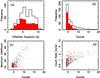 |
Fig. 1 Characteristics of the 487 sources comprising the XSS hard-band selected sample. Panel a) distribution of the effective exposure time of the full sample. The filled (red) histogram corresponds to the subset of XSS sources which were detected only in the XSS hard band. Panel b) distribution of the net counts recorded in the hard (2–10 keV) band (after background subtraction). The filled (red) histogram again corresponds to the hard-band only sources. Panel c) net counts versus the maximum likelihood of the detection with the hard-band only sources plotted in red. Panel d) net counts versus the corresponding count rate in ct/s with the hard-band only sources plotted in red. For clarity the 20 sources with net hard counts in the range 20–70 are not shown in Panels b)–d). |
2.2. Concurrent hard- and soft-band detection
In addition to the 2–10 keV measurements, the XSS also provides soft band (0.2–2 keV) data. Just over half (254 sources out of 487) of the hard-band selected sources were also detected simultaneously in the XSS soft band. Figure 2 shows a comparison of the count rates measured in the two XSS bands for the sources in our sample. In this figure the lower and upper diagonal lines represent soft:hard count-rate ratios of 1:1 and 10:1 respectively. For a source spectral model comprising a power-law continuum with Γ = 1.7 subject to soft X-ray absorption equivalent to NH = 3 × 1020 cm-2 (the fiducial spectral form on which the count rate to flux calibration is based), the soft to hard count-rate ratio is ≈ 2.7. This ratio increases to over 10 for Γ ≈ 2.5; similarly it drops to below 1 if the column density is increased to NH ≈ 5 × 1021 cm-2 (for Γ = 1.7).
2.3. False detections in the XSS
A survey which extends to sources with only 4 net counts, measured against a low but not entirely negligible background, will include some false detections arising from Poissonian noise spikes. In the case of the XSS sample one would expect the vast majority of the false detections to reside amongst the sources detected only in the hard band (since the probability of a simultaneous false detection in both the hard and soft bands will be very small). It is certainly true that the subset of “hard-band only” sources has a somewhat stronger weighting towards low net counts than the sources detected in both bands (see Fig. 1b). Specifically, 130 out of 233 (56%) of the hard-band only sources have between 4–5 net hard-band counts compared to 64 out of 254 (25%) for the dual-band detections.
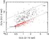 |
Fig. 2 XSS soft-band (0.2–2 keV) count rate versus the hard band (2–10 keV) count rate. Sources detected in both the hard and soft bands are plotted as squares, whereas those for which the soft-band measurement is an upper limit (corresponding to 4 net counts) are shown as (red) pluses. Error bars are shown for one high and one low-count rate source for illustration. The dotted diagonal lines correspond to soft to hard count-rate ratios of 1:1 and 10:1. |
To obtain an estimate of what fraction of the 233 XSS sources detected only in the hard-band might actually be spurious detections, we have applied the following argument. If we crudely approximate the source detection process (ignoring any issues relating to the background subtraction) as a search for groupings of N or more counts within a source cell of radius R = 20′′, then there are approximately 1.4 × 10⁸ such cells over the full XSS survey region. The typical background count in such a cell, based on the actual backgrounds measured in the XSS images, was in the range 0.01–0.05 counts, for which the Poissonian probability of measuring N ≥ 4 is roughly 1.0 × 10⁻⁷ (applying a weighted average over the background distribution). This implies the detection of just 14 spurious sources. The predicted false detection rate increases rapidly with R, with R = 30′′ giving roughly 150 false detections (although this is probably an over-estimate of the effective source cell size). A further observation is that the low-count sources are not preferentially drawn from slew datasets with higher than average background; this suggests that if there is a high false detection rate amongst such sources, then its origin is not solely due to Poissonian background fluctuations.
As a further test we randomised the photon distribution in a subset of the slew survey images and reran the source search algorithm. After applying the same selection criteria as employed in the current study, the number of spurious source detections, scaled to the full XSS area, was 33. However, we note that this approach does not encompass all of the complexities of the source detection within the XSS.
We will return to this issue when we consider the high number of “unidentified” sources amongst the subset of sources detected only in the XSS hard band.
2.4. Bias against the detection of extended sources
Some of the difficulties relating to the detection of extended sources in the low-exposure, low-count regime of the XSS have been discussed by Saxton et al. (2008). In practice, these issues translate to a fairly strong bias against the inclusion of extended objects within the current XSS sample. This selection bias will particularly impact on X-ray sources associated with nearby clusters of galaxies, which form a substantial fraction of the high-latitude source population seen in all-sky surveys such as Uhuru, Ariel V, and HEAO-1.
In selecting our XSS sample we imposed an upper limit on the extent parameter of 15 pixels (≈ 60′′). However, when we relax this selection criterion, the total number of sources in the sample only increases by six, none of which are obvious cluster candidates. Given this outcome, it is clear that the bias against extended objects is an intrinsic feature of the XSS.
To illustrate the magnitude of the problem, we have employed the complete sample of high-latitude (| b| > 20°) sources detected by the HEAO 1 A-2 experiment in the 2–10 keV band (Piccinotti et al. 1982) as a comparator. This sample (which we hereafter refer to as the Piccinotti sample) comprises 68 sources, 30 of which are identified as clusters of galaxies. We have investigated whether the XSS encompasses the positions of each of the Piccinotti sources and, where there is coverage, whether a hard-band detection resulted. For the non-detections we have gone back to the slew-survey data and determined an upper limit using a Bayesian-based on-line tool (Saxton & Gimeno 2011).
The results of this investigation were as follows. Ten of the Piccinotti clusters were covered by the XSS (up to and including XMMSL1d2). Of these 3 appear in our current sample with extent parameters in the range 3–14 pixels. A further HEAO 1 A-2 cluster was detected with an extent parameter of 20 pixels (but in the event this source did not make it into the XSS “clean” sample which was the starting point of our selection process). The X-ray fluxes derived for these 4 objects from the XSS were comparable (within a factor ~2) with those measured by the HEAO 1 A-2 experiment. The remaining 6 clusters were not detected with upper-limits (assuming point-like sources) between 3–30 times lower than those predicted from the HEAO 1 A-2 fluxes. As a further comparison the same analysis carried out for the 12 AGN in the Piccinotti sample covered by the XSS gave 10 detections plus 2 upper-limits with inferred variability factors typically in the range 1–3.
We conclude from this analysis that a strong bias does exist against the detection of extended objects in the XSS.
3. Counterparts to the XSS sources
3.1. Identification process
The next step was to draw together the available multiwaveband information relating to the likely counterparts of the sources in our XSS hard-band selected sample. The starting point was the cross-correlation of the XSS positions with other source catalogues encompassing a wide wavelength range. Saxton et al. (2008) quote the typical astrometric uncertainty of XSS positions to be 8′′ (the 68% confidence error radius), but for the purpose of cross-correlation with other catalogues, we initially adopted a search radius of 30′′. This process relied heavily on the facilities of Vizier3, supplemented by reference to Simbad4 and NED5. A few catalogues not currently available at Vizier were also accessed directly from the survey websites, the most notable being the Sloan Digital Sky Survey SDSS6 and the Galaxy Evolution Explorer (GALEX)7 source catalogues. In a preliminary pass we made a judgement on the likely identification of the X-ray source, if any. In the great majority of cases this involved consideration of the available information for a single putative counterpart, although in a small number of instances it was necessary to select the most likely counterpart amongst two or three candidates (using criteria such as the offset from the X-ray position and the brightness of the sources).
This first iteration separated the XSS sample into six broad categories. Sources of likely extragalactic origin were flagged as either AGN, Galaxies or Clusters (of galaxies). In general sources were categorized as Galaxies rather than AGN when there was a report of an extended optical/IR morphology and/or an associated redshift, but no definitive confirmation of the presence of an active nucleus. Similarly objects of likely Galactic origin were divided into Stars (mostly nearby objects with active stellar coronae) and Other categories (including X-ray binaries, cataclysmic variables supernova remnants and one pulsar). X-ray sources most likely residing in Local Group galaxies (M31, LMC and SMC) were also assigned to the Other category, as was an ultraluminous x-ray source (ULX) detected in NGC 2403. Finally the XSS sources without an obvious counterpart were categorized as Unidentified.
Subsequent iterations allowed the refinement of the above process using the knowledge derived from the earlier cycle. In particular, the great majority of the sources categorized as either the AGN, Galaxies or Stars were found to have both near-IR and mid-IR counterparts in the 2MASS8 and WISE9 surveys respectively. This allowed both the astrometric precision of the XSS and the IR colours of the counterparts to be explored in a systematic way. One application of the latter was to resolve some initial ambiguity as to whether the likely counterpart was a galaxy or a star on the basis of its IR colour (see Sect. 4.2). Also by exploiting the GALEX survey (Martin et al. 2005), which currently provides UV coverage of roughly two-thirds of the sky in the near-UV (NUV, 1350–1750 Å) and far-UV (FUV, 1750–2750 Å) bands, a number of sources initially categorized as Galaxies were switched to AGN on the basis of their UV to near-IR colour (Sect. 4.1).
An important consideration emerged in relation to the subset of XSS sources which were detected only in the hard X-ray band. Hereafter we refer to this subset as the “hard-only” sources, as opposed to the “hard+soft” sources detected simultaneously in both XSS bands. For the hard-only sources the success rate in finding relatively bright, plausible counterparts within a nominal search radius proved to be surprisingly low. As a consequence, in searching for putative counterparts down to fainter magnitudes, the rate of chance coincidences emerged as a crucial issue. In the event it proved necessary to focus on the hard-only sources with reasonable position errors as defined by the XSS pos_err10. As a practical approach the 68 hard-only sources with pos_err >10′′ were excluded from the identification statistics, although in practice there were very few plausible counterparts amongst this group. As a further step rather tight constraints were placed on the positional offsets and limiting magnitudes of the objects considered to be plausible counterparts to the remaining hard-only sources (see Sect. 3.3 for further details).
A summary of the final identification statistics for the full XSS sample is provided in Table 1, where the division is into the six broad source categories defined earlier. Table 1 also provides the identification information split down to the hard+soft and hard-only source subsets.
Division of the XSS sample into source types.
3.2. Counterparts of the XSS hard+soft sources
We first consider the identification statistics for the XSS sources detected simultaneously in both the XSS hard and soft bands (Table 1, Col. 3). A striking result is potential counterparts can be identified for all of these sources. Rather as expected, AGN predominate, whereas the number of clusters is small, consistent with our earlier discussion of the strong bias against extended sources in the XSS survey.
Within the hard+soft subset, 227 sources (out of 254) are categorized as either AGN, Galaxies or Stars. Of these, 223 appear in the WISE catalogue. For the four remaining sources, potential identifications were found in the GALEX catalogue (3 sources) or in 2MASS (a bright star); hence we have a complete set of counterpart positions for the AGN, Galaxies and Stars. The distribution of the angular offsets between the XSS position and the counterpart position is shown in Fig. 3. From this distribution one can conclude that the XSS 68% error radius is at ≈ 6′′ (which may be compared to the earlier estimate of 8′′ quoted by Saxton et al. 2008) and the 90% XSS error radius is at ≈ 10′′. Beyond 10′′ the offset distribution exhibits a long tail (Fig. 3), which might perhaps point to some of the identifications being incorrect. By way of illustration, consider the three most extreme outliers for which the putative counterpart is offset from the XSS position by >20′′. In these cases, the proposed counterparts (1 star, 1 galaxy and 1 AGN) are all relative bright WISE sources and are the only candidates visible within 30′′ of the X-ray position. Assuming that in these cases and in the others comprising the tail of the offset distribution, we do have the correct identification, then it would appear that the XSS position determination is occasional subject to atypical systematic errors (of up to 20′′), the origin of which are unknown.
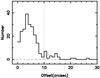 |
Fig. 3 X-ray to counterpart positional offsets for the XSS hard+soft sources classed as either AGN, Galaxies or Stars. The dotted vertical line is drawn at 10′′ and represents a nominal 90% error circle radius. |
As noted previously, the great majority of sources classed as either AGN, Galaxies or Stars have counterparts visible in both the 2MASS near-IR and the WISE mid-IR catalogues. There are in fact 213 hits with 2MASS and 223 with WISE out of a total sample of 227 objects. Figure 4 shows the resulting magnitude distributions for both the 2MASS J band and the WISE W1 (3.4 μm) band, with the contribution of objects classed as Stars highlighted. Clearly nearby stars dominate at bright magnitudes in both the near- and mid-IR. The broad J magnitude distribution of the coronally active stars detected in the XSS, with a shallow peak around J = 5–8, is in line with the much fainter (J ≈ 13–16) population of such objects discovered serendipitously in pointed XMM-Newton observations at X-ray flux levels ~103 times fainter than those reached in the XSS (see Warwick et al. 2011). The overlap region, between the stars on the one hand and AGN/galaxies on the other, extends over roughly 5 mag in both the J and W1 bands demonstrating that the apparent brightness of the counterpart is not a particularly effective method of distinguishing between Galactic and extragalactic counterparts. The peak in magnitude distribution for the AGN and Galaxies is well above the limiting sensitivity of both the 2MASS and WISE surveys, indicating that at the X-ray flux levels sampled by the XSS, these two surveys provide an ideal starting point for source identification.
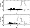 |
Fig. 4 Upper panel: the 2MASS J magnitude distribution of the counterparts to the XSS hard+soft sources categorized as either AGN, Galaxies or Stars. Lower panel: the WISE W1 (3.4 μm) magnitude distribution for the same source classes. In both panels the contribution of the Stars is highlighted as the filled histogram. |
3.3. Counterparts of the XSS hard-only sources
It is immediately evident from Table 1 (Col. 4) that the success rate in finding potential identifications for the XSS sources detected solely in the hard band is very much lower than that of sources detected simultaneously in both the XSS bands. The large number of sources which remain unidentified in the hard-only subset clearly merits some investigation.
A first consideration is that the XSS hard-only sources will have poorer position determinations than the hard+soft by virtue of the smaller number of counts available for the position determination algorithm (we employ the “best” XSS positions which, in most cases, derive from all the available counts for any given source). As noted earlier, to mitigate the impact of the poorer positions, we excluded hard-only sources with pos_err > 10′′ from the identification statistics. The net effect of the pos_err constraint was to reduce the hard-only sample from 233 sources to 165 sources. For comparison, if the same filter were to be applied to the hard+soft sources this would lead to the removal of just 8 sources, 5 of which lie in the Clusters category.
Even with the reduced sample, a large fraction of the hard-only sources remain unidentified (110 out of 165, i.e. two-thirds of the sample). With so many unidentified sources, it was essential to take account of the chance coincidence rate when searching for potential counterparts down to relatively faint fluxes. To quantify this we investigated the probability of finding an object within a nominal 10′′ error circle as a function of the limiting magnitude for both the 2MASS J and the WISE W1 bands. In both cases the chance rates were determined by searching for the brightest object within a 10′′ circle positioned at a set of grid points around each XSS source location (with an offset from the actual X-ray position always >1′). The results are shown in Fig. 5. It is evident that at the survey limit, the WISE W1 band probes a source density ≈ 2.6 times higher than that reached in the 2MASS J band. Therefore, in the analysis below, we use the WISE survey as our yardstick for determining the chance coincidence rate.
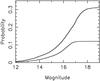 |
Fig. 5 The probability of finding by chance an object brighter than a given magnitude within a 10′′ radius error circle. The upper curve corresponds to the WISE W1 (3.4 μm) band and the lower curve to the 2MASS J band. |
Setting aside the 10 sources in the Other category, we conducted a systematic search for the counterparts to the hard-only sources using the WISE survey. For putative counterparts brighter than W1 = 12 we extended the search radius to 20′′, whereas for objects in the range W1 = 12–15 we restricted the radius to 10′′ (noting that the latter equates to the 90% error radius for the hard+soft sources). Candidate objects fainter than W1 = 15 were not considered. The number of potential counterparts as a function of the W1 magnitude emerging from this process is listed in Table 2, together with an estimate of the number of source expected by chance across the 165 sources comprising the (reduced) hard-band only sample. In total 45 potential counterparts were found – as reported in Table 1. The corresponding number of chances coincidences was predicted to be 10.6. We note from Table 2 that at the faint end of the magnitude range considered, the chance rate is rapidly approaching the actual number of objects found. We conclude, that a limiting W1 magnitude of ≈ 15 and a search radius at faint fluxes of no more than 10 ′′ defines a reasonable bound to counterpart searches for the hard-only XSS sample.
Incidence of potential WISE counterparts amongst the 165 sources comprising the (reduced) hard-only sample as a function of the W1 (3.4 μm) magnitude.
Of the 45 hard-only sources classed as AGN, Galaxies or Stars, only 2 fall in the latter category. This presumably reflects the fact that coronally active stars generally have soft thermal spectra and are not subject to significant line-of-sight absorption (particularly when detected at high Galactic latitude). The split between AGN and Galaxies is also much more strongly weighted to the latter in the hard-only sample. This could be the result of absorbing material within the host galaxy suppressing both the soft X-ray emission and also masking the AGN character of the source at longer wavelengths.
This leaves us with some uncertainty as to the nature of the numerous unidentified sources in the hard-only sample. If one applies the same filtering to the hard+soft identification as applied to the hard-only sources (pos_err < 10′′, W1 < 15, search radii as in Table 2), then the number of sources (AGN, Galaxies and Stars) with putative WISE counterparts drops from 233 to 205, i.e., a modest 12% decrease. It would seem that the unidentified sources amongst the hard-only sample, if real, must represent a population of astrophysical sources substantially fainter than found amongst the XSS hard+soft subset. However, there is no real evidence for the emergence of such a population down to W1 = 15, which is 3 mag fainter than the peak of distribution in Fig. 4. One might speculate that the unidentified sources correspond to infrequent, relatively short-lived outbursts linked to an otherwise underluminous source population, but in truth they are difficult to match to any known class of X-ray emitting object (see also Sect. 5.2). Unfortunately, a follow-up study of a subset of XSS sources with Swift provided no information contrary to the above analysis (Starling et al. 2011).
The alternative possibility is that a great many of the unidentified sources are not real astrophysical sources, but rather false detections, mostly at the 4-count threshold. The argument against this hypothesis is that the numbers of sources involved exceed the estimates of Sect. 2.3 by a factor of at least 3. However, given the nature of the XSS, a higher than predicted false detection rate is certainly a possibility. At the very least some caution is needed when dealing with XSS sources detected only in a single band at the 4-count limit.
Division into source types in the XSS extragalactic sample.
4. The XSS extragalactic sample
4.1. Composition of the sample
We may now use the source identifications to construct an XSS extragalactic sample. To this end, we have included the sources classed as either AGN or Galaxies in Table 1, but excluded Clusters given the strong bias against such sources in the XSS. Our full XSS extragalactic sample comprises 219 sources. Details of the individual sources are provided in the appendix (Table A.1), where we list the counterpart position, source type and redshift (if known).
The composition of the extragalactic sample is presented in Table 3 for the full set of sources and also split between the hard+soft and hard-only subsets. Here the AGN are grouped according to their spectroscopic classification, as taken from the literature. As noted earlier a number of sources initially categorized as Galaxies were switched to AGN on the basis of their UV to near-IR colour. The specific requirement was for NUV – J < 5, where NUV is the near-UV magnitude from GALEX and the J magnitude is from the 2MASS. The 18 objects that met this criterion are classed as UVX sources both in Tables 3 and A.1.
Of the 219 AGN and galaxies comprising the XSS extragalactic sample, 181 have spectroscopic or photometrically estimated redshifts (see Table A.1). The distribution of redshifts is shown in Fig. 6. The mode of the distribution is at z ≈ 0.05; for a source at the survey limit the corresponding X-ray luminosity (for H0 = 70 km s-1 Mpc-1) is ~1.7 × 1043 erg s-1 (2–10 keV).
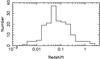 |
Fig. 6 Redshift distribution of the sources in the XSS extragalactic sample. Redshifts are known for 181 out of the 219 sources which comprise the sample. |
4.2. Infrared colours
We have investigated the mid-IR and near-IR colours of the AGN and galaxies in the XSS extragalactic sample by utilising the WISE 3.4, 4.6, 12 and 22 μm data (i.e., the W1, W2, W3 and W4 bands respectively), and the 2MASS J, H and K bands. Mid-IR and near-IR two-colour diagrams are shown in Fig. 7. These diagrams demonstrate that the AGN and galaxies are well separated from the stellar coronal sources in terms of their W2 − W3 colour (apart from one or two early type stars found in local star formation regions). With slightly less efficiency, the H − K colour also serves to distinguish between the extragalactic and Galactic X-ray source populations. We note that the sources in the XSS extragalactic sample occupy largely the same region of the mid-IR two-colour diagram as the luminous AGN in the Bright Ultra-Hard XMM-Newton Survey (Mateos et al. 2012).
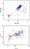 |
Fig. 7 The mid- and near-IR colours of the AGN and galaxies in the XSS extragalactic sample. Top panel: WISE W2 − W3 versus W3 − W4 two-colour diagram. Bottom panel: 2MASS J − H versus H − K two-colour diagram. In both cases, the XSS AGN are shown as crosses (black) and the galaxies as circles (blue). For comparison, the XSS sources categorized as stars are shown as asterisks (red). |
4.3. Cross-correlation with the Swift BAT catalogue
We have also investigated the coincidence of the XSS extragalactic sample with sources discovered in the hard (14–195 keV) X-ray band by the BAT experiment on Swift. For this purpose we use the on-line11Swift BAT 58-Month Hard X-ray Survey (Baumgartner et al. 2010). Using a 1′ search radius, there were 37 XSS-BAT matches, 6 of which were with XSS hard-only sources. Figure 8 shows the correlation diagram for the 14–195 keV versus 2–10 keV fluxes, in which diagonal dotted lines delineate 14–195 keV:2–10 keV flux ratios of 1:1 and 10:1. For comparison, the lower ratio applies to a source exhibiting relatively soft continuum emission (Γ ~ 2) subject to a modest level of absorption (NH ≈ 1021 cm-2), whereas a requisite for the higher ratio is either a very hard continuum (Γ ~ 1.0) or substantial line-of-sight absorption (NH > 1023 cm-2).
Interestingly there were no BAT detections of any of the XSS sources classed as Unidentified.
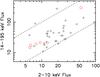 |
Fig. 8 The correlation between the 14–195 keV flux (10-12 erg cm-2 s-1) measured by the BAT experiment on Swift and the XSS 2–10 keV flux (10-12 erg cm-2 s-1) for the 37 cross matches. XSS hard+soft are shown as crosses, whereas XSS hard-only sources are shown as circles (red). The dotted lines represent BAT:XSS flux ratios of 1:1 and 10:1 respectively. |
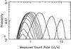 |
Fig. 9 Probability of measuring a given output count rate for simulated sources of fixed input count rate. These probability density functions are based on bins of 0.05 ct/s width and are smoothed versions of the raw simulation data (using a 1-d top-hat smoothing filter with a width of 5 bins). From left to right (based on the position of the peak) the curves correspond to input count rates of 0.1, 0.2, 0.3, 0.4, 0.5, 0.6, 0.7, 0.8, 1.0, 2.0, 5.0 and 10 ct/s. For this plot the normalisation of the 0.1 ct/s curve has been scaled upwards by a factor of 5. |
5. Determination of the XSS source counts
A major objective of this investigation was to establish the log N − log S relation for a sample of extragalactic sources selected in the hard 2–10 keV from the XSS and to compare the results with those reported from other surveys. Given the small numbers of clusters detected in the XSS, the focus is necessarily on the identified sample of AGN and galaxies.
5.1. The results from a Monte Carlo simulation
Given the wide range of factors which might influence the detection probability of real sources and, for those sources with positive detections, might deviate the measured count rate from the true value, we have carried out a Monte Carlo simulation of the survey process.
In brief, this involved adding simulated sources at random positions to the set of sky images created as part of the slew survey pipeline. For a simulated source of specified count rate, the number of net counts was calculated on the basis of the effective exposure and then randomised according to Poissonian statistics. These counts were then distributed about the assigned source position according to the appropriate point spread function. The source detection algorithm was then applied and the number of counts net of the background determined from which a measured count rate could be assigned. The simulated source was classed as a detection and considered further provided all the criteria applied in the actual XSS selection were met (e.g., a minimum of 4 net counts). Repetition of this process then allowed a count rate probability distribution appropriate to the specified input rate to be determined. Finally a series of trials were conducted so as to cover a representative range of input count rate; each of these trials were based on 10 000 simulated sources, except for the two trials at the lowest input count rates (0.1 and 0.2 ct/s) where 20 000 sources were employed and the trial with the highest input rate (10 ct/s) which was based on 4000 sources.
Figure 9 shows the results of the simulation in the form of probability density curves plotted as a function of the measured count rate. The set of curves cover two decades of input count rate from 0.1 ct/s up to 10 ct/s. The detection probability evidently truncates at a measured count rate of ~0.4 ct/s, i.e., the 4 count threshold divided by the maximum exposure of ≈ 10 s. We note that even at very low input rates (e.g., 0.2 ct/s for which the average count at maximum exposure is 2), there is still a finite probability that the source will be detected, since Poissonian deviations allow the occasional detection of the source at or above the 4 count threshold.
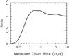 |
Fig. 10 Ratio of the predicted differential log N − log S function (as determined by the simulation) to the assumed input power-law form. |
The next step was to use the curves in Fig. 9 to predict the number of sources detected as a function of the measured count rate. Here we took the underlying differential log N − log S function of the cosmic X-ray source population to be a powerlaw function with index γ and normalisation K: 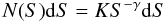 (1)where S is the true count rate in ct/s units and N(S)dS is the number of sources with true count rate in the range S to S + dS. We assumed γ = 2.5 (i.e., the Euclidean form of the source counts).
The range S = 0.1–20 ct/s was divided into bins (of width 0.01 ct/s for S = 0.10–0.25 ct/s and 0.1 ct/s thereafter) and the number of sources ΔN within the bin calculated. For each value of S the corresponding probability density P(Sm) as a function of the measured count rate, Sm was determined, where necessary by interpolating across the curves shown in Fig. 9. The summation of the ΔN × P(Sm) products over the full range of S then allowed the differential source count as a function of the measured count rate, M(Sm), to be determined.
The ratio M(Sm))/N(Sm) is then a prediction, based on the simulation, of how closely the measured source counts will track the input form. Figure 10 shows this ratio for the range of count rates encompassed by our XSS sample. The simulation demonstrates the onset of a cutoff below a measured count rate of 1 ct/s with a sharp truncation at ≈ 0.4 ct/s. The prediction of a slight excess of sources with measured count rates from 1–3 ct/s most likely stems from the effect of Eddington bias. This is the process by which, through Poissonian fluctuations, faint sources are boosted to higher levels more frequently than bright sources are suppressed, by virtue of the numerical superiority of the former.
Further evidence of the major impact of Eddington bias on the XSS is provided in Fig. 11 which shows the spread in the true (input) count rate for sources detected at a particular measured count rate. For example, a measured count rate of 0.5 ct/s can derive from sources with true count rate anywhere between 0.1–1 ct/s. Even for much brighter sources the underlying uncertainty in the true count rate (and hence the source flux) is surprisingly large.
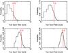 |
Fig. 11 Spread in the true (input) count rate for sources detected at different measured count rates. The four panels show the results for measured count rates of 0.5, 1.0, 2.0 and 5.0 ct/s (as represented by the vertical lines). |
5.2. Extragalactic log N – log S relation
We have determined the source counts of the set of sources which comprise our extragalactic sample. A technical issue arises in relation to how to deal with the overlap of the XMM-Newton slews which comprise the XSS. As noted earlier, this overlap results in some duplicate source detections in the primary XSS database, which we subsequently removed in building our hard-band selected sample. However, the source count calculation is greatly simplified if we ignore this overlapping coverage, but commensurately add back the duplicate detections. In practice this involved adding 17 duplication detections to the set of 219 sources which comprise our extragalctic sample.
The integral source counts were determined by giving each source a weight N(Sm)/M(Sm) (i.e., the reciprocal of the function plotted in Fig. 10) and then summing these weights as a function of decreasing Sm. The result is shown in Fig. 12 in a normalised form, i.e., the measured integral counts divided by the integral version of the fiducial Euclidean source count defined previously.
The integral log N − log S curve for the extragalactic sources follows the Euclidean form below 3.0 ct/s. The normalisation implies 100 sources brighter than 1 ct/s are detected in the 14 233 square degree covered by the XSS (overlaps included), which, down to the limiting sensitivity of the XSS (0.4 ct/s = 3.2 × 10⁻¹² erg cm-2 s-1) implies ~1000 X-ray sources in the high-latitude sky above |b| > 10° (excluding, of course, clusters of galaxies and Galactic objects). In Fig. 12 there is an apparent deficit of sources above 3.0 ct/s. In fact using the normalisation quoted above and assuming the Euclidean form for the counts extends from 3–10 ct/s, we predict 14 sources in this count rate range compared to the 9 sources in the actual sample. For a Poisson distribution, the chances of recording 9 or less events for a mean rate of 14 is 11%, implying that the deficit of bright sources in the XSS is not hugely significant.
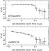 |
Fig. 12 Top panel: integral log N − log S curve for the extragalactic XSS sample (excluding clusters of galaxies) normalised to N(>S) = 100 × S-1.5. Bottom panel: integral log N − log S curve for the sources classed as Unidentified in the XSS hard-band selected sample. |
By way of comparison, Fig. 12 also shows the integral counts for the 178 sources classed as Unidentified in the XSS hard-band selected sample. The steep form of this relation (γ ≈ 3.0) is difficult to match to any known astrophysical population and hence adds weight to the conjecture that most of these sources are spurious.
We have also derived the differential form of the log N − log S curve for the extragalactic sample. Figure 13 shows the result, again normalised to the Euclidean form. So as to make comparisons with other surveys, we have converted the XSS count rates to 2–10 keV fluxes using the conversion factor specified in Sect. 2.1. As noted above, within the flux range encompassed by the XSS, the counts of extragalactic objects (excluding clusters) follow the Euclidean form. Figure 13 also compares the XSS results with the differential 2–10 keV source counts at high latitude derived from the 2XMM catalogue (Mateos et al. 2008). The normalisation of the source counts at the high flux end of the 2XMM survey and at the low flux end of the XSS are very comparable, suggesting that a smooth interpolation is possible across the intervening gap (which amounts to a factor ~3 in flux). There is, however, the caveat that the 2XMM data do not specifically exclude either Galactic interlopers or clusters of galaxies. Figure 13 also shows a point at high flux corresponding to the AGN sample defined by Piccinotti et al. (1982) on the basis of the HEAO-1 A2 survey. Here the agreement with XSS is good, apart from the apparent deficit in the highest XSS bin12.
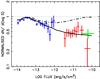 |
Fig. 13 Differential 2–10 keV log N − log S curve for the XSS extragalactic sample (red data points), normalised to the Euclidean form. At the faint end the XSS results are compared with the differential 2–10 keV source counts derived from the 2XMM catalogue by Mateos et al. (2008) (blue points). At the bright end the comparison is with the HEAO-1 A2 AGN sample of Piccinotti et al. (1982) (green point). The solid curve is the prediction of the AGN source counts from the work of Gilli et al. (2007). The dot-dashed curve similarly represents the prediction of the total extragalactic counts, i.e., AGN plus clusters of galaxies. In drawing these comparisons account has been taken of the relevant survey sky areas. In this plot the normalisation factor has been matched to the counts of the AGN plus clusters at the high flux end. |
To aid the interpretation of the source counts we have also plotted in Fig. 13, the predictions of Gilli et al. (2007) for the 2–10 keV band both for AGN alone and for AGN plus clusters of galaxies. There is clearly excellent agreement between the AGN prediction and the measured XSS counts. In the flux range of the XSS, we might expect that the inclusion of clusters in the extragalactic sample would result in an additional 80–100% of sources (consistent with the Piccinotti et al results where clusters represented half the total extragalactic sample). Clearly this reemphasises the point made earlier that there is a very strong selection bias against extended sources in the XSS catalogue. Figure 13 also provides at least a hint that some clusters of galaxies may also be missing from the 2XMM catalogue (Mateos et al. 2008).
6. Summary and conclusions
The substantial sky coverage afforded by the XSS makes this survey a unique resource for studying X-ray bright source samples. We have shown that, with care, the XSS can be used to define reliable subsets of sources selected in the 2–10 keV band, down to a limiting sensitivity of 3 × 10-12 erg cm-2 s-1 and encompassing sources with as few as 4 counts net of the background. One caveat is that there is a significant bias against the detection of extended sources, such as clusters of galaxies. A second caveat is that a significant fraction (≈ 75%) of the faint XSS sources detected solely in the hard band may in fact be spurious detections.
For the purpose of source identification, the XSS is well matched to currently available all-sky IR surveys such as 2MASS and WISE. For the XSS sources detected simultaneously in the XSS hard and soft bands, the hit rate with WISE was close to 100%, in the case of the AGN/galaxies and stellar coronal emitters. The infrared colours of the counterparts also provides a rather efficient method of removing the active stars when constructing an extragalactic sample. Unfortunately, for the XSS sources detected only in the hard band, the search for WISE counterparts is somewhat compromised by the high chance rate that applies when the sample size is inflated by spurious detections.
A major motivation of this work was to use the XSS to determine the extragalactic log N − log S relation in a flux regime which is poorly sampled by existing surveys. To that end we constructed an XSS extragalactic sample comprised of 219 sources with likely identifications as AGN/galaxies, but necessarily excluding clusters of galaxies. Using the results of a detailed simulation of the source detection procedure we were able to apply corrections for the complex selection biases which come into play in the low-count regime of the XSS. The conclusion of this study was that the normalisation we derive for the XSS extragalactic source counts fits well with published measurements at brighter and fainter levels, which together span 4 decades in X-ray flux.
Online material
Appendix A:
Details of the sources which comprise the hard-band selected XSS extragalactic sample are given in Table A.1. The table provides the following information for each source: the XSS name; whether the source was also detected in the XSS soft band; the XSS hard band (2−10 keV) flux and error on the flux (in units of 10-11 erg cm-2 s-1); the RA and Dec of the proposed counterpart; the name of the counterpart; the type of the counterpart; the redshift (if known). The table is available as a FITS file from the authors.
Sources comprising the XSS extragalactic sample.
For a source to be included in our sample we require a detection maximum likelihood (maxl) in the XSS hard band of either maxl > 10, if the background count rate was less than 3 ct/s, or maxl > 14 otherwise. These are the same criteria as used to define the “clean” XSS sample, except now applied specifically to the hard band. Note that in the on-line XSS catalogue the maxl parameter has the designation DET_ML.
Note that a duplicate detection of Mrk 421 at a count rate less than the 10 ct/s upper threshold, restored this source to our final sample.
The Two Micron All Sky Survey (2MASS) (Cutri et al. 2003; Skrutskie et al. 2006) provides uniform coverage of the entire sky in three near-infrared (NIR) bands, namely in J (1.25 μ), H (1.65 μ) and Ks (2.17 μ).
The Wide Field Infrared Explorer (WISE) has recently observed the entire sky at 3.4, 4.6, 12 and 22 μm. The All-SKY Data Release covers >99% of the sky and incorporates the best available calibrations and data reduction algorithms (Cutri et al. 2012).
The pos_err parameter provides an estimate of the uncertainty of the XSS position, albeit a rather crude one for sources at the low-count threshold. In the present work we restrict its use to filtering out the hard-only sources with particularly poor position determinations. Note that in the on-line XSS catalogue the pos_err parameter has the designation RADEC_ERR.
Available at http://heasarc.nasa.gov/docs/swift/results/bs58mon/
In this case roughly 4 additional sources would be required in the highest flux bin (encompassing sources with count rates from 5–10 ct/s) so as to raise this bin to an ordinate value of 0.5.
Acknowledgments
A.M.R. acknowledges STFC/UKSA funding support. We thank Silvia Mateos for providing the 2XMM source count data in a convenient form. This research has made use of the SIMBAD and Vizier facilities at CDS, Strasbourg and the NASA/IPAC Extragalactic Database (NED). This publication utilises data from the Two Micron All Sky Survey, which is a joint project of the University of Massachusetts and IPAC/Caltech. This paper has also made use of the source catalogue from the Wide-field Infrared Survey Explorer, which is a NASA sponsored joint project of the University of California, Los Angeles, and the Jet Propulsion Laboratory/California Institute of Technology. Use was also made of data from the Galaxy Evolution Explorer, GALEX, which is operated for NASA by the California Institute of Technology under NASA contract NAS5-98034. The XMM-Newton project is an ESA science mission with instruments and contributions directly funded by ESA member states and the USA (NASA).
References
- Alexander, D. M., Bauer, F. E., Brandt, W. N., et al. 2003, AJ, 126, 539 [NASA ADS] [CrossRef] [Google Scholar]
- Baumgartner, W. H., Tueller, J., Markwardt, C., & Skinner, G. 2010, BAAS, 41, 675 [Google Scholar]
- Brunner, H., Cappelluti, N., Hasinger, G., et al. 2008, A&A, 479, 283 [NASA ADS] [CrossRef] [EDP Sciences] [Google Scholar]
- Comastri, A., Ranalli, P., Iwasawa, K., et al. 2011, A&A, 526, L9 [NASA ADS] [CrossRef] [EDP Sciences] [Google Scholar]
- Cutri, R. M., Skrutskie, M. F., van Dyk, S., et al. 2003, Explanatory Supplement to the 2MASS All-Sky Data Release and Extended Mission Products (Pasadena: IPAC/Caltech) [Google Scholar]
- Cutri, R. M., Wright, E. L., Conrow, T., et al. 2012, Explanatory Supplement to the WISE All-Sky Data Release Products (Pasadena: IPAC/Caltech) [Google Scholar]
- Elvis, M., Civano, F., Vignali, C., et al. 2009, ApJS, 184, 158 [NASA ADS] [CrossRef] [Google Scholar]
- Forman, W., Jones, C., Julien, P., et al. 1978, ApJS, 38, 357 [NASA ADS] [CrossRef] [Google Scholar]
- Gilli, R., Comastri, A., & Hasinger, G. 2007, A&A, 463, 79 [NASA ADS] [CrossRef] [EDP Sciences] [Google Scholar]
- Giommi, P., Perri, M., & Fiore, F. 2000, A&A, 362, 799 [Google Scholar]
- Luo, B., Bauer, F. E., Brandt, W. N., et al. 2008, ApJS, 179, 19 [NASA ADS] [CrossRef] [Google Scholar]
- Martin, D. C., Fanson, J., Schiminovich, D., et al. 2005, ApJ, 619, L1 [Google Scholar]
- Mateos, S., Warwick, R. S., Carrera, F. J., et al. 2008, A&A, 492, 51 [NASA ADS] [CrossRef] [EDP Sciences] [Google Scholar]
- Mateos, S., Alonso-Herro, A., Carrera, F. J., et al. 2012, MNRAS, in press [Google Scholar]
- McHardy, I. M., Lawrence, A., Pye, J. P., & Pounds, K. A. 1981, MNRAS, 197, 893 [NASA ADS] [CrossRef] [Google Scholar]
- Piccinotti, G., Mushotzky, R. F., Boldt, E. A., et al. 1982, ApJ, 253, 485 [Google Scholar]
- Saxton, R. D., & Gimeno, C. D.-T. 2011, ASPC, 442, 567 [NASA ADS] [Google Scholar]
- Saxton, R. D., Read, A. M., Esquej, M. P., et al. 2008, A&A, 480, 611 [NASA ADS] [CrossRef] [EDP Sciences] [Google Scholar]
- Skrutskie, M. F., Cutri, R. M., Stiening, R., et al. 2006, AJ, 131, 1163 [NASA ADS] [CrossRef] [Google Scholar]
- Starling, R. L. C., Evans, P. A., Read, A. M., et al. 2011, MNRAS, 412, 1853 [NASA ADS] [CrossRef] [Google Scholar]
- Ueda, Y., Ishisaki, Y., Takahashi, T., Makishima, K., & Ohashi, T. 2005, ApJS, 161, 185 [NASA ADS] [CrossRef] [Google Scholar]
- Voges, W., Aschenbach, B., Boller, T., et al. 1999, A&A, 349, 389 [NASA ADS] [Google Scholar]
- Warwick, R. S., Pérez-Ramírez, D., & Byckling, K. 2011, MNRAS, 413, 595 [NASA ADS] [CrossRef] [Google Scholar]
- Watson, M. G., Schröder, A. C., Fyfe, D., et al. 2009, A&A, 493, 339 [NASA ADS] [CrossRef] [EDP Sciences] [Google Scholar]
- Wood, K. S., Meekins, J. F., Yentis, D. J., et al. 1984, ApJS, 56, 507 [NASA ADS] [CrossRef] [Google Scholar]
- Xue, Y. Q., Luo, B., Brandt, W. N., et al. 2011, ApJS, 195, 10 [NASA ADS] [CrossRef] [Google Scholar]
All Tables
Incidence of potential WISE counterparts amongst the 165 sources comprising the (reduced) hard-only sample as a function of the W1 (3.4 μm) magnitude.
All Figures
|
Fig. 1 Characteristics of the 487 sources comprising the XSS hard-band selected sample. Panel a) distribution of the effective exposure time of the full sample. The filled (red) histogram corresponds to the subset of XSS sources which were detected only in the XSS hard band. Panel b) distribution of the net counts recorded in the hard (2–10 keV) band (after background subtraction). The filled (red) histogram again corresponds to the hard-band only sources. Panel c) net counts versus the maximum likelihood of the detection with the hard-band only sources plotted in red. Panel d) net counts versus the corresponding count rate in ct/s with the hard-band only sources plotted in red. For clarity the 20 sources with net hard counts in the range 20–70 are not shown in Panels b)–d). |
| In the text | |
|
Fig. 2 XSS soft-band (0.2–2 keV) count rate versus the hard band (2–10 keV) count rate. Sources detected in both the hard and soft bands are plotted as squares, whereas those for which the soft-band measurement is an upper limit (corresponding to 4 net counts) are shown as (red) pluses. Error bars are shown for one high and one low-count rate source for illustration. The dotted diagonal lines correspond to soft to hard count-rate ratios of 1:1 and 10:1. |
| In the text | |
|
Fig. 3 X-ray to counterpart positional offsets for the XSS hard+soft sources classed as either AGN, Galaxies or Stars. The dotted vertical line is drawn at 10′′ and represents a nominal 90% error circle radius. |
| In the text | |
|
Fig. 4 Upper panel: the 2MASS J magnitude distribution of the counterparts to the XSS hard+soft sources categorized as either AGN, Galaxies or Stars. Lower panel: the WISE W1 (3.4 μm) magnitude distribution for the same source classes. In both panels the contribution of the Stars is highlighted as the filled histogram. |
| In the text | |
|
Fig. 5 The probability of finding by chance an object brighter than a given magnitude within a 10′′ radius error circle. The upper curve corresponds to the WISE W1 (3.4 μm) band and the lower curve to the 2MASS J band. |
| In the text | |
|
Fig. 6 Redshift distribution of the sources in the XSS extragalactic sample. Redshifts are known for 181 out of the 219 sources which comprise the sample. |
| In the text | |
|
Fig. 7 The mid- and near-IR colours of the AGN and galaxies in the XSS extragalactic sample. Top panel: WISE W2 − W3 versus W3 − W4 two-colour diagram. Bottom panel: 2MASS J − H versus H − K two-colour diagram. In both cases, the XSS AGN are shown as crosses (black) and the galaxies as circles (blue). For comparison, the XSS sources categorized as stars are shown as asterisks (red). |
| In the text | |
|
Fig. 8 The correlation between the 14–195 keV flux (10-12 erg cm-2 s-1) measured by the BAT experiment on Swift and the XSS 2–10 keV flux (10-12 erg cm-2 s-1) for the 37 cross matches. XSS hard+soft are shown as crosses, whereas XSS hard-only sources are shown as circles (red). The dotted lines represent BAT:XSS flux ratios of 1:1 and 10:1 respectively. |
| In the text | |
|
Fig. 9 Probability of measuring a given output count rate for simulated sources of fixed input count rate. These probability density functions are based on bins of 0.05 ct/s width and are smoothed versions of the raw simulation data (using a 1-d top-hat smoothing filter with a width of 5 bins). From left to right (based on the position of the peak) the curves correspond to input count rates of 0.1, 0.2, 0.3, 0.4, 0.5, 0.6, 0.7, 0.8, 1.0, 2.0, 5.0 and 10 ct/s. For this plot the normalisation of the 0.1 ct/s curve has been scaled upwards by a factor of 5. |
| In the text | |
|
Fig. 10 Ratio of the predicted differential log N − log S function (as determined by the simulation) to the assumed input power-law form. |
| In the text | |
|
Fig. 11 Spread in the true (input) count rate for sources detected at different measured count rates. The four panels show the results for measured count rates of 0.5, 1.0, 2.0 and 5.0 ct/s (as represented by the vertical lines). |
| In the text | |
|
Fig. 12 Top panel: integral log N − log S curve for the extragalactic XSS sample (excluding clusters of galaxies) normalised to N(>S) = 100 × S-1.5. Bottom panel: integral log N − log S curve for the sources classed as Unidentified in the XSS hard-band selected sample. |
| In the text | |
|
Fig. 13 Differential 2–10 keV log N − log S curve for the XSS extragalactic sample (red data points), normalised to the Euclidean form. At the faint end the XSS results are compared with the differential 2–10 keV source counts derived from the 2XMM catalogue by Mateos et al. (2008) (blue points). At the bright end the comparison is with the HEAO-1 A2 AGN sample of Piccinotti et al. (1982) (green point). The solid curve is the prediction of the AGN source counts from the work of Gilli et al. (2007). The dot-dashed curve similarly represents the prediction of the total extragalactic counts, i.e., AGN plus clusters of galaxies. In drawing these comparisons account has been taken of the relevant survey sky areas. In this plot the normalisation factor has been matched to the counts of the AGN plus clusters at the high flux end. |
| In the text | |
Current usage metrics show cumulative count of Article Views (full-text article views including HTML views, PDF and ePub downloads, according to the available data) and Abstracts Views on Vision4Press platform.
Data correspond to usage on the plateform after 2015. The current usage metrics is available 48-96 hours after online publication and is updated daily on week days.
Initial download of the metrics may take a while.