| Issue |
A&A
Volume 548, December 2012
|
|
|---|---|---|
| Article Number | A51 | |
| Number of page(s) | 13 | |
| Section | Astronomical instrumentation | |
| DOI | https://doi.org/10.1051/0004-6361/201015689 | |
| Published online | 20 November 2012 | |
A comparison of algorithms for the construction of SZ cluster catalogues
1 DSM/Irfu/SPP, CEA/Saclay, 91191 Gif-sur-Yvette Cedex, France
e-mail: jean-baptiste.melin@cea.fr
2 Institut d’Astrophysique Spatiale, CNRS et Université de Paris XI, Bâtiment 120-121, Centre Universitaire d’Orsay, 91400 Orsay Cedex, France
3 Institut fur Theoretische Astrophysik, Zentrum fur Astronomie der Universitat Heidelberg, Albert-Ueberle-Str. 2, 69120 Heidelberg, Germany
4 APC, 10 rue Alice Domon et Léonie Duquet, 75205 Paris Cedex 13, France
5 Université Paris Diderot – Paris 7, 75205 Paris Cedex 13, France
6 Jet Propulsion Laboratory, California Institute of Technology, 4800 Oak Grove Drive, Pasadena, CA 91109, USA
7 DSM/Irfu/SAp, CEA/Saclay, 91191 Gif-sur-Yvette Cedex, France
8 Astrophysics Group, Cavendish Laboratory, J.J. Thomson Avenue, Cambridge, CB3 0HE, UK
9 Max-Planck-Institut für extraterrestrische Physik Giessenbachstr, 85748 Garching, Germany
10 Instituto de Física de Cantabria (CSIC-UC), 39005 Santander, Spain
11 Kavli Institute for Cosmology Cambridge and Institute of Astronomy, Madingley Road, Cambridge, CB3 OHA, UK
12 ALMA JAO, Av. El Golf 40 – Piso 18, Las Condes, Santiago ;
ESO, Alonso de Córdova 3107, Vitacura, Casilla 19001, Santiago, Chile
13 Università di Roma “Tor Vergata”, via della ricerca scientifica, 1, 00133 Roma, Italy
14 Astronomisches Rechen-Institut, Monchhofstrasse 12-14, 69120 Heidelberg, Germany
15 Dipartimento di Astronomia, Università di Bologna, via Ranzani 1, 40127 Bologna, Italy
Received: 3 September 2010
Accepted: 3 October 2012
We evaluate the construction methodology of an all-sky catalogue of galaxy clusters detected through the Sunyaev-Zel’dovich (SZ) effect. We perform an extensive comparison of twelve algorithms applied to the same detailed simulations of the millimeter and submillimeter sky based on a Planck-like case. We present the results of this “SZ Challenge” in terms of catalogue completeness, purity, astrometric and photometric reconstruction. Our results provide a comparison of a representative sample of SZ detection algorithms and highlight important issues in their application. In our study case, we show that the exact expected number of clusters remains uncertain (about a thousand cluster candidates at |b| > 20 deg with 90% purity) and that it depends on the SZ model and on the detailed sky simulations, and on algorithmic implementation of the detection methods. We also estimate the astrometric precision of the cluster candidates which is found of the order of ~2 arcmin on average, and the photometric uncertainty of about 30%, depending on flux.
Key words: cosmology: observations / galaxies: clusters: general / galaxies: clusters: intracluster medium / cosmic background radiation / methods: data analysis
© ESO, 2012
1. Introduction
Galaxy cluster catalogues have played a long-standing, vital role in cosmology, providing important information on topics ranging from cosmological parameters to galaxy formation (Rosati et al. 2002; Voit 2005). In particular, recent X-ray cluster catalogues have proved valuable in establishing the standard cosmological model (e.g., Schuecker et al. 2003; Vikhlinin et al. 2009). The science potential of large cluster surveys is strong: They are, for instance, considered one of the central observational tools for illuminating the nature of dark energy (e.g., the Dark Energy Task Force Report Albrecht et al. 2006, 2009). A suite of large cluster surveys planned over the coming years in the optical/IR, X-ray and millimeter bands will greatly extend the reach of cluster science by probing much larger volumes to higher redshifts with vastly superior statistics and control of systematics.
The Planck SZ cluster catalogue will be one of the important players in this context. Surveying the entire sky in 9 millimeter/submillimeter bands with ~5–10 arcmin resolution over the channels most sensitive to the cosmic microwave background (CMB) anisotropies, the Planck satellite will find large numbers of clusters through the Sunyaev-Zel’dovich (SZ) effect (Sunyaev & Zeldovich 1970, 1972; Birkinshaw 1999; Carlstrom et al. 2002). The advantages of this, much anticipated, technique include efficient detection of distant clusters and selection based on an observable expected to correlate tightly with cluster mass (Bartlett 2002; da Silva et al. 2004; Motl et al. 2005; Nagai 2006; Bonaldi et al. 2007; Shaw et al. 2008). An official mission deliverable, the Planck SZ catalogue will be the first all-sky cluster catalogue since the workhorse catalogues from the ROSAT All-Sky Survey (RASS, Truemper1992), in other words, Planck will be the first all-sky cluster survey since the early 1990s!
Within the Planck Consortium, a considerable effort has been conducted for the scientific evaluation of the cluster catalogue construction methodology. As part of this evaluation effort, we completed an extensive comparison of twelve algorithms applied to detailed simulations of Planck data based on the Planck Sky Model (PSM). This study was dubbed “The SZ Challenge” and was carried out in two steps using different SZ cluster models and cosmologies; these are referred to as Versions 1 and 2 and more fully explained below. We report the findings of these initial studies in terms of catalogue completeness and purity, as well as astrometric and photometric accuracy and precision.
The article is organized as follows: In the next section we detail our sky simulations, including a brief description of their basis, the PSM (Delabrouille et al. 2012). The following section then introduces the different catalogue construction methodologies employed, before moving on to a presentation of each of the twelve algorithms in the study. We present the results of the challenge in Sect. 4, followed by a comparative study of algorithmic performance. We conclude with a discussion of both the limitations of this study and future directions.
2. Simulations
2.1. The Planck Sky Model
One of the important differences between the present work and previous studies of Planck SZ capabilities is the detailed and rather sophisticated simulation of millimeter and submillimeter sky emission used here. Our sky simulations are based on an early development version of the PSM (Delabrouille et al. 2012), a flexible software package developed within the Planck Collaboration for making predictions, simulations and constrained realisations of the microwave sky. The simulations used for this challenge are not polarised (only temperature maps are useful for detecting clusters using the thermal SZ effect).
The CMB sky is based on the best fit angular power spectrum model of WMAP. The CMB realisation is not constrained by actual observed CMB multipoles, in contrast to the simulations used by Leach et al. (2008).
Diffuse Galactic emission is described by a four component model of the interstellar medium comprising free-free, synchrotron, thermal dust and spinning dust and is based on Miville-Deschênes et al. (2008, see Miville-Deschênes 2009, for a review). The predictions rely on a number of sky templates with different angular resolutions. In order to simulate the sky at Planck resolution we have added small-scale fluctuations to some of the templates to increase the fluctuation level as a function of the local brightness and therefore reproduce the non-Gaussian and non-uniform properties of the interstellar emission. The procedure used to add small scales is presented in Miville-Deschênes et al. (2007).
Free-free emission is based on the model of Dickinson et al. (2003) assuming an electronic temperature of 7000 K. The spatial structure of the emission is modeled using an Hα template corrected for dust extinction. The Hα map is a combination of the Southern H-Alpha Sky Survey Atlas (SHASSA, Gaustad et al. 2001) and the Wisconsin H-Alpha Mapper (WHAM, Haffner et al. 2003), smoothed to obtain a uniform angular resolution of 1°. Dust extinction is inferred using the E(B − V) all-sky map of Schlegel et al. (1998). As mentioned earlier, small scales were added in both templates to match the Planck resolution. The free-free emission law is constant over the sky, as it depends only on the electronic temperature, taken as a constant here (see however Wakker et al. 2008, for a description of high-velocity clouds not detected by the WHAM survey and hence not included in our simulations).
Synchrotron emission is based on an extrapolation of the 408 MHz map of Haslam et al. (1982) from which an estimate of the free-free emission was removed. In any direction on the sky, the spectral emission law of the synchrotron is assumed to follow a power law,  . We use a pixel-dependent spectral index β derived from the ratio of the 408 MHz map and the estimate of the synchrotron emission at 23 GHz in the wmap data obtained by Miville-Deschênes et al. (2008).
The thermal emission from interstellar dust is estimated using model 7 of Finkbeiner et al. (1999). This model, fitted to the FIRAS data (7° resolution), assumes that each line of sight can be modeled by the sum of the emission from two dust populations, one cold and one hot. Each grain population is in thermal equilibrium with the radiation field and thus has a grey-body spectrum, so that the total dust emission is modelled as  (1)where Bν(Ti) is the Planck function at temperature Ti. In model 7 the emissivity indices are β1 = 1.5, β2 = 2.6, and f1 = 0.0309 and f2 = 0.9691. Once these values are fixed, the dust temperature of the two components is determined using only the ratio of the observations at 100 μm and 240 μm. For this purpose, we use the 100/240 μm map ratio published by Finkbeiner et al. (1999). Knowing the temperature and β of each dust component at a given position on the sky, we use the 100 μm brightness at that position to scale the emission at any frequency using Eq. (1).
Characteristics of instrumental values taken from Planck blue book for a 14 month nominal mission.
Spinning dust emission uses as a template the dust extinction map E(B − V), and uses an emission law uniform on the sky, based on the model of Draine & Lazarian (1998), assuming a warm neutral medium (WNM).
We emphasise that the emission laws of both synchrotron and dust vary across the sky. The spectral index of free-free and the emission law of spinning dust, however, are taken as uniform on the sky.
Point sources are modeled with two main categories: radio and infrared. In the present simulation, none of two is correlated with the SZ signal. Simulated radio sources are based on the NVSS or SUMSS and GB6 or PMN catalogues. Measured fluxes at 1 and/or 4.85 GHz are extrapolated to 20 GHz using their measured SED when observed at two frequencies. Sources for which a flux measurement is available at a single frequency have been randomly assigned to either the steep- or to the flat-spectrum class in the proportions observationally determined by Fomalont et al. (1991) for various flux intervals, and assigned a spectral index randomly drawn from the corresponding distribution. Source counts at 5 and 20 GHz obtained in this way are compared, for consistency, with observed counts, with the model by Toffolatti et al. (1998), and with an updated version of the model by de Zotti et al. (2005), allowing for a high-redshift decline of the space density of both flat-spectrum quasars (FSQs) and steep-spectrum sources (not only for FSQs as in the original model). Further extrapolation at Planck frequencies has been made allowing a change in SED above 20 GHz, assuming again a distribution in flat and steep populations. For each of these two populations, the spectral index is randomly drawn within a set of values compatible with the typical average and dispersion. Infrared sources are based on the iras catalogue, and modeled as dusty galaxies (Serjeant & Harrison 2005). IRAS coverage gaps were filled by randomly adding sources with a flux distribution consistent with the mean counts. Fainter sources were assumed to be mostly sub-millimeter bright galaxies, such as those detected by SCUBA surveys. These were modelled following Granato et al. (2004) and assumed to be strongly clustered, with a comoving clustering radius r0 ≃ 8 h-1 Mpc. Since such sources have a very high areal density, they are not simulated individually but make up the sub-mm background.
The SZ component is described in detail in the following section.
Component maps are produced at all Planck central frequencies. They are then co-added and smoothed with Gaussian beams as indicated in Table 1, extracted from the Planck blue book. We thus obtain a total of nine monochromatic sky maps.
Finally, inhomogeneous noise is simulated according to the pixel hit count corresponding to a nominal 14-month mission1 using the Level-S simulation tool (Reinecke et al. 2006). The rms noise level in the simulated maps is given in Table 1 from the Planck blue book. It is worth noting that the in-flight performances of Planck-HFI as reported by the Planck Collaboration (Planck Collaboration 2011a) are better than the requirements.
2.2. The SZ component
We simulate the SZ component using a semi-analytic approach based on an analytic mass function dN(M,z)/dMdz. After selecting cosmological parameters (h, Ωm, ΩΛ, σ8), the cluster distribution in the mass-redshift plane (M,z) is drawn from a Poisson law whose mean is given by the mass function. Clusters are spanning the mass range 5×10¹³ M⊙ < Mvir < 5×10¹⁵ M⊙ and the redshift range 0 < z < 4. Cluster Galactic coordinates (l,b) are then uniformly drawn on the sphere. We compute the SZ signal for each dark matter halo following two different models, producing two simulations (v1 and v2) with different sets of cosmological parameters and mass functions and SZ signals2.
2.2.1. SZ challenge v1
For the first version of the SZ Challenge, we used h = 0.7, Ωm = 0.3, ΩΛ = 0.7, σ8 = 0.85 and the Sheth-Tormen mass function Sheth & Tormen (1999). We assume that the clusters are isothermal and that the electron density profile is given by the β-model, with β = 2/3, and core radius scaling as M1/3. We truncate the model at the virial radius, rvir, and choose the core radius rc = rvir/10. The virial radius here is defined according to the spherical collapse model. The temperature of each cluster is derived using a mass-temperature given in Colafrancesco et al. (1997) with T15 = 7.75 keV, consistent with the simulations of Eke et al. (1998). For more details on this model, we refer the reader to Sect. 5 of de Zotti et al. (2005).
2.2.2. SZ challenge v2
The second version of the SZ Challenge was produced using a WMAP5 only cosmology (Dunkley et al. 2009) (h = 0.719, Ωm = 0.256, ΩΛ = 0.744, σ8 = 0.798). We used the Jenkins mass function (Jenkins et al. 2001). The SZ emission is modeled using the universal pressure profile derived from the X-ray REXCESS cluster sample (Arnaud et al. 2010) which predicts profile and normalisation of SZ clusters given their mass and redshift. The profile is well fitted by a generalized NFW profile that is much steeper than the β-profile in the outskirts. Moreover, for a given mass, the normalisation of the SZ flux is ~ 15% lower than the normalisation of SZ Challenge v1. This profile was used as the baseline profile in the SZ early results from Planck (Planck Collaboration 2011b,f,e,c,g).
Neither of the two sets of simulations (v1 and v2) contains point sources within clusters. The effect of contamination by radio or infrared point sources in clusters was therefore not studied here3. We neither include relativistic electronic populations within clusters. As for point sources, this effect was not studied here4.
3. Methods and algorithms
The SZ Challenge was run as a blind test by providing the simulated sky maps. Participating teams, ten, were then asked to run their algorithms, twelve in total on the simulated data and supply a cluster catalogue with
-
1.
(α,δ): cluster sky coordinates;
-
2.
Yrec: recovered total SZ flux, in terms of the integrated Compton-Y parameter;
-
3.
ΔYrec: estimated flux error, i.e., the method’s internal estimate of flux error;
-
4.
θrec: recovered cluster angular size, in terms of equivalent virial radius;
-
5.
Δθrec: estimated size error (internal error).
The different methods were divided into two classes: direct methods that produce a cluster catalogue applying filters directly to a set of frequency maps, and indirect methods that first extract a thermal SZ map and then apply source finding algorithms.
In this classification, the 12 algorithms studied were:
-
Direct methods:
-
MMF1: matched multi-filters (MMF) as implemented byHarrison.
-
MMF2: MMF as described in Herranz et al. (2002).
-
MMF3: MMF as described in Melin et al. (2006).
-
MMF4: MMF as described in Schäfer et al. (2006).
-
PwS: Bayesian method PowellSnakes as described in Carvalho et al. (2009).
-
-
Indirect methods:
-
BNP: Bayesian Non-parametric method as describedin Diegoet al. (2002), followed bySExtractor (Bertin & Arnouts 1996) to detectclusters and perform photometry.
-
ILC1: All-sky internal linear combination (ILC) on needlet coefficients5 (similar to the method used for CMB extraction in Delabrouille et al. 2009) to get an SZ map, followed by matched filters on patches to extract clusters and perform photometry.
-
ILC2: Same SZ map Delabrouille et al. (2009), but followed by SExtractor on patches instead of a matched filter to extract the clusters. Photometry or flux measurement is however done using matched filters at the position of the detected clusters.
-
ILC3 developed by Chon and Kneissl: ILC in real space and filtering in harmonic space to obtain an SZ map, followed by fitting a cluster model.
-
ILC4 developed by Melin: ILC on patches in Fourier space to obtain SZ maps, followed by SExtractor to detect clusters and matched multifilters to perform photometry.
-
ILC5 developed by Yvon: ILC on patches in wavelet space to obtain SZ maps, followed by SExtractor to detect clusters and perform photometry.
-
GMCA: Generalized Morphological Component Analysis as described in Bobin et al. (2008), followed by wavelet filtering and SExtractor to extract clusters and matched multifilters to perform photometry.
-
Summary of the algorithms compared in the SZ Challenge.
3.1. Matched multifilter methods
The multifrequency matched filter (MMF) enhances the contrast (signal-to-noise) of objects of known shape and known spectral emission law over a set of observations containing correlated contamination signals. It offers a practical way of extracting a SZ clusters using multifrequency maps. The method makes use of the universal thermal SZ effect frequency dependance (assuming electrons in clusters are non-relativistic), and adopts a spatial (angular profile) template. The filter rejects foregrounds using a linear combination of maps (which requires an estimate of the statistics of the contamination) and uses spatial filtering to suppress both foregrounds and noise (making use of prior knowledge of the cluster profile). In all cases discussed here, the adopted template is identical to the simulated cluster profiles, except for MMF2 on SZ Challenge v2. The MMF has been studied extensively by Herranz et al. (2002) and Melin et al. (2006).
Three of the MMF methods tested here work with projected flat patches of the sky, and one method works directly on the pixelised sphere.
In the first case, the full-sky frequency maps are projected onto an atlas of overlapping square flat regions. The filtering is then implemented on sets of small patches comprising one patch for each frequency channel. For each such region, the nine frequency maps are processed with the MMF. A simple thresholding detection algorithm is used to find the clusters and produce local catalogues. The MMF is applied with varying cluster sizes to find the best detection for each cluster. This provides an estimate of the angular size in addition to the central Compton parameter. Each algorithm explored its own, but similar, range of angular scales; MMF3, for example, runs from θv = 2 to 150 arcmins. The catalogues extracted from individual patches are then merged into a full-sky catalogue that contains the position of the clusters, their estimated central Compton parameter, the virial radius and an estimation of the error in the two later quantities. The integrated Compton parameter is derived from the value of the central Compton parameter and the radius of the cluster.
In the following, we give relevant details specific to each implementation of the MMF.
3.1.1. MMF1
The performance of the MMF1 algorithm is sensitive to the accuracy of the evaluation of the power spectra and cross-power spectra of the non-SZ component of the input maps. The detection is performed in two passes, the first detecting the highest signal-to-noise SZ clusters, and the second detecting fainter clusters after the removal of the contribution of the brightest ones from the power spectra estimated on the maps.
The merging of the catalogues from distinct patches is implemented with the option of discarding detections found in the smallest radius bin. These detections essentially correspond to spatial profiles indistinguishable from that of a point source. This option permits better control of the contamination by point sources, as a disproportionate fraction of the spurious detections occur in this bin ; despite their different spectral signature, point sources can occasionally pass through the filter. Using this option of MMF1 reduces the contamination at a given threshold (see Sect. 4.1 for definitions of this and other diagnostics of catalogue content) depending on the actual profile of the SZ clusters.
3.1.2. MMF2
The MMF2 algorithm follows closely the method described in Herranz et al. (2002). The method is simple and quite robust, although the performance depends on the model assumed for the radial profile of the clusters. For this work, a truncated multiquadric profile similar to a β-model has been used for SZ Challenge v1 and v2. The profile is not a good match for the simulated profile in SZ Challenge v2. This does not affect significantly the completeness and purity of the method (as shown in Sect. 4) but the extracted flux is biased with respect to the input. The family of profiles used by the algorithm can however be adjusted.
3.1.3. MMF3
The MMF3 SZ extraction algorithm is an all-sky extension of the matched multifrequency filter described in Melin et al. (2006). It has been used for the production of the early SZ cluster sample (Planck Collaboration 2011b). In the version used for the SZ challenge, auto and cross power spectra used by the filter do not rely on prior assumptions about the noise, but are directly estimated from the data. They are thus adapted to the local instrumental noise and astrophysical contamination.
3.1.4. MMF4
The spherical matched and scale adaptive filters (Schäfer et al. 2006) are generalisations of the filters proposed by Herranz et al. (2002) for spherical coordinates. Just like their counterparts they can be derived from an optimisation problem and maximise the signal to noise ratio while being linear in the signal (matched filter) and being sensitive to the size of the object. The algorithm interfaces to the common HEALPIX package and treats the entire celestial sphere in one pass.
The most important drawback is the strong Galactic contamination – the filter was not optimised to deal with a Galactic cut like many of the other algorithms, although it is in principle possible to include that extension. The large noise contribution due to the Galaxy is the principal reason why the performance of the filter suffers in comparison to the approach of discarding a large fraction of the sky.
3.2. Bayesian methods
3.2.1. PowellSnakes
PowellSnakes (PwS; Carvalho et al. 2009) is a fast multi-frequency Bayesian detection algorithm. It analyses flat sky patches using the ratio  (2)where H1 is the detection hypothesis, “There is a source” and H0 the null hypothesis “Only background is present” (Jaynes 2003). Applying Bayes theorem to the above formula one gets
  (3)where
  (4)is the evidence, ℒ(Θ) is the likelihood, π(Θ) is the prior and Θ a vector representing the parameter set.
An SZ parameterised template profile of the clusters s(X,A) ≡ ξ τ(a, x − X, y − Y), is assumed known and fairly representative of the majority of the clusters according to the resolution and signal-to-noise ratio of the instrumental setup, where τ(...) is the general shape of the objects (beta or Arnaud et al. profile) and aj a vector which contains the parameters controlling the geometry of one specific element (core/scale radius, parameters of the beta or Arnaud et al. profile).
The algorithm may be operated on either “Frequentist mode” where the detection step closely resembles a multi-frequency multi-scale “matched filter” or “Bayesian mode” where the posterior distributions are computed resorting to a simple “nested sampling” algorithm (Feroz & Hobson 2008).
The acceptance/rejection threshold may be defined either by using “Decision theory” where the expected loss criterion is minimised or by imposing a pre-defined contamination ratio. In the case of a loss criterion, the symmetric criterion – “An undetected cluster is as bad as spurious cluster” – is used.
3.2.2. BNP
This method is described in detail in Diego et al. (2002). It is based on the maximization of the Bayesian probability of having an SZ cluster given the multifrequency data with no assumptions about the shape nor size of the clusters. The method devides the sky into multiple patches of about 100 sq. degrees and performs a basic cleaning of the Galactic components (by subtracting the properly weighted 857 GHz map from the channels of interest for SZ) and point sources (using a Mexican Hat Wavelet). The cleaned maps are combined in the Bayesian estimator and the output map of Compton parameters is derived. SExtractor is applied to the map of reconstructed Compton parameter to detect objects above a given threshold and compute their flux. The thresholds are based on the background or noise estimated by SExtractor. In order to compute the purity, different signal-to-noise ratios (ranging from 3 to 10) are used to compute the flux. The method assumes a power spectrum for the cluster population although this is not critical.
The main advantage of the method resides in its robustness (almost no assumptions) and its ability to reconstruct both extended and compact clusters. The main limitation is the relatively poor reconstruction of the total flux of the cluster as compared to matched filters.
3.3. Internal linear combination methods
The ILC is a simple method for extracting one single component of interest out of multifrequency observations. It has been widely used for CMB estimation on WMAP data (Bennett et al. 2003; Tegmark et al. 2003; Eriksen et al. 2004; Park et al. 2007; Delabrouille et al. 2009; Kim et al. 2009; Samal et al. 2009). A general description of the method can be found in Delabrouille & Cardoso (2009).
The general idea behind the ILC is to form a linear combination of all available observations which has unit response to the component of interest, while minimizing the total variance of the output map. This method assumes that all observations yi(p), for channel i and pixel p, can be written as the sum of one single template of interest scaled by some coefficient ai, and of unspecified contaminants which comprise noise and foregrounds, i.e.  (5)where yi(p) is the observed map in channel i, s(p) is the template of interest (here, the SZ map), and ni(p) comprise the contribution of both all astrophysical foregrounds (CMB, galactic emission, point sources...) and of instrumental noise. This equation can be recast as:
  (6)To first order, linear combinations of the inputs of the form ∑ iwiyi(p) guarantee unit response to the component of interest provided that the constraint ∑ iwiai = 1 is satisfied (there are, however, restrictions and higher order effects, which are discussed in detail in the appendix of Delabrouille et al. 2009; Dick et al. 2010). It can be shown straightforwardly (Eriksen et al. 2004; Delabrouille & Cardoso 2009) that the linear weights which minimize the variance of the output map are:
  (7)where
  is the empirical covariance matrix of the observations. What distinguishes the different ILC implementations is essentially the domains over which the above solution is implemented.
3.3.1. ILC1
The needlet ILC method works in two steps. First, an SZ map is produced by ILC, with a needlet space implementation similar to that of Delabrouille et al. (2009). The use of spherical needlets permits the ILC filter to adapt to local conditions in both direct (pixel) space and harmonic space. Input maps include all simulated Planck maps, as well as an external template of emission at 100 microns (Schlegel et al. 1998), which helps subtracting dust emission. The cluster catalogue is then obtained by matched filtering on small patches extracted from the needlet ILC SZ full-sky map, as described in Melin et al. (2006).
3.3.2. ILC2
The ILC2 approach relies on the same processing for photometry, cluster size, and signal-to-noise estimates as in ILC1, but in this case the detection of cluster candidates is made using SExtractor on a Wiener-filtered version of the ILC1 map.
While the extraction of the ILC map works on full sky maps, using the needlet framework to perform localized filtering, here again the detection of cluster candidates, and the estimation of size and flux, are performed on small patches (obtained by gnomonic projection).
3.3.3. ILC3
In this method, a filter in the harmonic domain is applied to construct a series of maps that are sensitive to the range of cluster scales. We used a Mexican-hat filter constructed from two Gaussians, one with 1/4 the width of the other. A list of cluster candidates is compiled using a peak finding algorithm, which searches for enhanced signal levels in the individual map by fitting cluster model parameter. We employed the β-model profile with β = 2/3 convolved with the Planck beams. The catalogue produced then includes as parameters the cluster location, the flux, and the size estimate. The errors on these parameters are incorporated as given by the likelihoods of the fit.
Additional improvements to the method can be achieved by using more optimal foreground estimators (but probably with slower convergence). This is useful especially for the fainter clusters, or those confused to a high degree by source contamination.
3.3.4. ILC4
The ILC4 method is a standard ILC in Fourier space performed on the square patches. It is implemented independently in annuli in wave number (modulus of the Fourier mode) by applying weights, according to Eq. (7), this time in the Fourier domain. The cluster detection is performed using SExtractor on the reconstructed SZ map. The flux estimation is performed on the original multifrequency maps (small patches) using the MMF at the position of the SExtractor detections.
3.3.5. ILC5
This algorithm is designed to work on local noisy multichannel maps in the wavelet domain. The representation of galaxy clusters in an appropriate biorthogonal wavelet basis is expected to be sparse compared to the contributions of other astrophysical components. This should ease the subsequent SZ separation using the ILC method at each wavelet scale. The reverse wavelet transform is then applied to estimate local SZ-maps. The latter are convolved using a Gaussian beam of 5 arcmin FWHM to reduce the noise prior to cluster detection using SExtractor with a threshold fixed classically to a multiple of the rms noise (signal-to-noise ratio ranging from 3 to 6). The brightest IR galaxies and radiosources are masked to reduce contamination. Finally, multiple detections due to the overlap of local maps are removed. Multiscale ILC proved to be more efficient than regular ILC to remove large angular scale contamination on local map simulations. However, the cluster catalogue appears comparatively more contaminated which may be due to an imperfect cleaning of multiple detections. Also, the known point sources were only masked before detection with SExtractor. Masking the observed sky maps earlier could improve the component separation using Multiscale ILC. Doing so may prevent a few very bright pixels biasing the ILC parameter estimation but in turn raises the question of data interpolation across masked regions. The other implementations of the ILC do mask point sources before combining the maps and are thus not subject to this bias.
3.4. GMCA
Generalized morphological component analysis is a blind source separation method devised for separating sources from instantaneous linear mixtures using the model given by: Y = AS + n. The components S are assumed to be sparsely represented (i.e. have a few significant samples in a specific basis) in a so-called sparse representation Φ (typically wavelets). Assuming that the components have a sparse representation in the wavelet domain is equivalent to assuming that most components have a certain spatial regularity. These components and their spectral signatures are then recovered by minimizing the number of significant coefficients in Φ:  (8)where ||...||2 is the L2 (Euclidean) norm. In Bobin et al. (2008), it was shown that sparsity enhances the diversity between the components thus improving the separation quality. The spectral signatures of CMB and SZ are assumed to be known. The spectral signature of the free-free component is approximately known up to a multiplicative constant (power law with fixed spectral index).
Hence, GMCA furnishes a noisy SZ map in which we want to detect the SZ clusters. This is done in three steps:
-
wavelet denoising;
-
SExtractor to extract the clusters from the noise-free SZ map, and finally;
-
a maximum likehood to get the flux of the detected sources.
4. Results
We evaluated each extracted catalogue in terms of catalogue content and photometric recovery based on comparisons between the extracted catalogues and the simulated input SZ cluster catalogue. For this purpose, we cut the input catalogue at Y > 5×10⁻⁴ arcmin2, well below the theoretical Planck detection limit (see below), and restrict ourselves to the high latitude sky at |b| > 20 deg to reduce contamination by galactic foregrounds. We then cross-match the candidate cluster in a given catalogue to a corresponding input cluster. Each match results in a true detection, while candidates without a match are labeled as false detections. In a second step, we compare the extracted properties, namely SZ Compton parameter and size, of the true detections to the input cluster properties.
Angular proximity was the only association criterion used for the matching. Specifically, we matched an extracted cluster to an input cluster if their separation on the sky θ < θmax = f(θv), a function of the true angular virial radius of the (input) cluster. The function f(θv) varied over three domains: f(θv) = 5 arcmin for θv < 5 arcmin; f(θv) = θv for 5 arcmin < θv < 20 arcmin; and f(θv) = 20 arcmin for θv > 20 arcmin.
We first focus on the catalogue completeness and purity, both of which we define immediately below. We then test the accuracy of the recovered flux and size estimates, as well as each algorithm’s ability to internally evaluate the uncertainties on these photometric quantities. Since many fewer codes ran on the Challenge v2, we focus mainly on Challenge v1. We include results for those codes that did run on Challenge 2 to gauge the influence of the underlying cluster model used for the simulation.
4.1. Catalogue content
A useful global diagnostic is the curve of yield versus global purity for a given catalogue (see e.g. Pires et al. 2006). The former is simply the total number of clusters detected and the latter we define as 1 − Γg, where Γg is the global contamination rate:  (9)The yield curve is parametrized by the effective detection threshold of the catalogue construction algorithm. It is a global diagnostic because it gauges the total content of a catalogue, rather than its content as a function of flux or other measurable quantities.
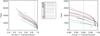 |
Fig. 1 For SZ Challenge v1: yield as a function of global purity. The right handside panel is a zoom on the high-purity region. Each curve is parameterized by the detection threshold of the corresponding algorithm. As discussed in the text, the overall value of the yields should be considered with caution, due to remaining modeling uncertainties (see text). We focus instead on relative yield between algorithms as a measure of performance. |
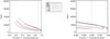 |
Fig. 2 For SZ Challenge v2: yield as a function of global purity. The same comment applies concerning the overall yield values; in particular, the cluster model changed significantly between the versions v1 and v2 of the Challenge resulting in lower overall yields here. Fewer codes participated in the Challenge v2 (see text). |
Figure 1 compares the yield curves of outputs of all the algorithms in the SZ Challenge v1, and Fig. 2 those for the SZ Challenge v2. Increasing the detection threshold moves a catalogue along its curve to higher purity and lower yield. Algorithms increase in performance towards the upper right-hand corner, i.e., both high yield and high purity.
As to be expected, algorithms that locally estimate the noise (both instrumental and astrophysical), i.e. on local patches of a few square degrees, perform much better than those that employ a global noise estimate, such as MMF4 and ILC3. For those methods with local noise estimation, we note that their effective survey depth appears to anticorrelate with the instrumental noise, indicating that astrophysical confusion is effectively removed. This can be seen in Fig. 3, which compares the density of detected SZ sources (top panel) to the pixel hit count (bottom panel). The result illustrated with one single method, ILC2 run on the SZ challenge v1, holds for the other algorithms. The cluster detection limit appears to be primarily modulated by the instrumental noise at high Galactic latitude, as opposed to foreground emission.
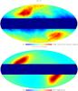 |
Fig. 3 Illustrated for ILC2 on the SZ Challenge v1, the detection density (top panel) is compared to the pixel hit count for the map at 143 GHz (bottom panel). The noise in the simulated Planck maps scales as 1/ |

Less expected, perhaps, is the fact that all algorithms tend to miss nearby clusters. These are extended objects, and although they have large total SZ flux, these clusters are “resolved-out” – missed because of their low surface brightness. This is an extreme example of resolution effects expected in the case of SZ detection in relatively low resolution experiments like Planck. It is not related to the foreground removing efficiency since the effect can also be mimicked in simulations including only instrumental white noise. Apart from the few clusters that are fully resolved, many have angular sizes comparable to the effective beam, and this leads to a non-trivial selection function (White 2003; Melin et al. 2005, 2006).
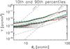 |
Fig. 4 Selection curves for each algorithm in the true Y–true θv plane for SZ Challenge v1. The lower set of curves indicate the 90th percentiles, i.e., the curve above which lie 90% of the detected clusters; the upper set corresponds to the 10th percentile. The colour codes are as in Fig. 1. We see that the Planck selection function depends not just on flux, but also on cluster angular size. Many clusters are at least marginally resolved by Planck, leading to these size effects in the selection fuction. The dashed lines show contours of fixed mass and redshift, as indicated, while the cloud of points shows the distribution of the input catalogue (in fact a subsample of 1 in 4 randomly selected input clusters). We see that small variations in selection curves generate significant yield changes. |
We emphasize that the numerical values of the yields depend on the cosmological model, on the foreground model and on the cluster model used in the simulations. They must be considered with caution because of the inherent modeling uncertainties. As for the foreground model, the templates used to model Galactic components in the PSM were chosen so that they are reasonably representative of the complexity of the diffuse galactic emission. Thanks to many new observations in particular in the IR and submm domain (Lagache et al. 2007; Viero et al. 2009; Hall et al. 2010; Amblard et al. 2011; Planck Collaboration 2011d), the models of point sources have evolved very much between the beginning of the SZ challenge and the publication of these results. These updates were not taken into account in the PSM when the study was performed. Moreover, the cluster model in challenge v1 was based on the isothermal β-model, while v2 employed a modified NFW pressure profile favoured by X-ray determinations of the gas pressure (Arnaud et al. 2010) with a normalization of the Y − M relation lower by ~15% than in v1. Finally, σ8 changed from 0.85 in challenge v1 to 0.796 in v2 which strongly influences the total cluster yield.
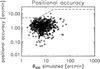 |
Fig. 5 Positional accuracy of the recovered clusters illustrated for MMF3 in the SZ challenge v2. |
The more peaked profile actually improves detection efficiency, while the lower normalization reduces the predicted yield. Along with the much lower value of σ8, the net result is that the yields in challenge v2 are noticeably lower than in v1 as seen in Figs. 1 and 2. We thus only discuss, in this study, the relative yields of the codes as a gauge of performance treating the absolute value of the yield with caution.
Focusing on the relative merit of the algorithms, we see that Figs. 1 and 2 display large dispersion in the yield at a given purity. This reflects of course the intrinsic performance of the algorithms, but also for the detection methods that share similar underlying algorithms, e.g. MMF and ILC, the dispersion in the yield reflects the differences in implementations (e.g. noise estimation, de-blending, etc.).
Somewhat deceptively, these yield variations correspond to only minor differences in detection threshold, as illustrated for the SZ Challenge v1 in Fig. 4. This figure traces the curves above which 90% and 10% (lower set and upper set respectively) of the clusters detected by each method lie in the true Y − true θv plane. As already mentioned, many clusters are marginally resolved (sizes at least comparable to the beam), which means that detection efficiency depends not only on flux, but also on size6.
The algorithms all have similar curves in this plane. This means that the differences in yield are due to only small variations of the selection curve since completeness is expected to be monotonic. The black points represent a random sample of 1/4 of the input clusters and show where the bulk of the catalogue lies. These small variations have important consequences for cosmological interpretation of the counts and hence must be properly quantified.
We compute for all the methods and in the SZ challenges v1 and v2 the completeness defined as the ratio [true detections (recovered clusters)/simulated clusters] over bins of true (simulated) flux Y. We find it varies from 80 to 98% at Ylim = 10-2 arcmin2 for the direct methods (based on frequency maps). The completness is of order of 80% at the same Ylim for the indirect methods (based on detections in SZ maps). We note a slight increase of the completeness from the SZ Challenge v1 to v2. We also estimate the contamination of the output catalogues defined as the ratio [false detections/total detections]. This is evaluated as as a function of recovered flux. The average contamination of the output catalogues ranges between 6 and 13% both in the case of the challenge 1 and 2. However, the purity with respect to the Y bins differ significantly from method to method. As a general trend, the lowest Y bin, i.e. the smallet recovered fluxes centred around 10-3 arcmin2, is more contaminated (~75% on average) in the case of the indirect method than in the case of direct methods (~50% on average).
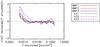 |
Fig. 6 Flux recovery bias. The figure shows for a subset of methods the average recovered Yrec, normalized to the true input Y, as a function of Y. At the bright end, most codes extract an unbiased estimate of cluster flux, while the expected Malmquist bias appears at the faint-end, just below Y ~ 2×10⁻³ arcmin2. |
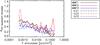 |
Fig. 7 Flux recovery uncertainty for the subset of methods given in Fig. 6. The Figure shows the dispersion in measured flux about the true input Y flux as a function of the true input flux. The best algorithms are affected by ~ 30% dispersion. |
4.2. Photometric and astrometric recovery
Cluster characterization is a separate issue from detection. It involves determination of angular positions as well as photometry. Since Planck will marginally resolve many clusters, photometry here means both flux Yrec and characteristic size measurements. Moreover, each method should provide an estimate of the errors on these quantities for each object in the catalogue.
We illustrate in Fig. 5, a scatter diagram of positional offset for MMF3 as a function of true cluster size, θv. On average, all the algorithms perform similarly and recover cluster position to ~2 arcmin with a large scatter. In addition, we see that it is more difficult to accurately determine the position of intrinsically extended clusters, as shown by the fact that the cloud of points is elongated and inclined.
Concerning photometry, we show in Figs. 6 and 7 the mean recovered SZ flux, Yrec, normalized to the true (simulated) flux, Y, as a function of the latter. Only true detections are used in this comparison. We illustrate our results for a subset of methods namely MMF1, MMF2, MMF3, ILC1, ILC2, ILC3. Methods that filter the maps such as ILC4 and GMCA, or that use the SExtractor photometry such as BNP and ILC5 exhibit significant bias in flux recovery at the bright end. At the faint end, we see the appearance of Malmquist bias as an upturn in the measured flux. The importance of this bias varies from algorithm to algorithm.
Figure 7 gives the dispersion in the recovered flux σYrec as a function of true Y (once again, only involving true detections). Here, we see that some codes perform significantly better than others. Those that adjust an SZ profile to each cluster outperform by a large margin those that do not. Photometry based on SExtractor, for example, fares much worse than the MMF codes. Even among the best performing codes, however, the intrinsic photometric dispersion is of order 30%. This is important, because we expect SZ flux to tightly correlate with cluster mass, with a scatter as low as ~10% as indicated by both numerical simulations (Kravtsov et al. 2006) and recent X-ray data (Arnaud et al. 2007; Nagai et al. 2007). The SZ flux hence should offer a good mass proxy. What we see from this figure, however, is that the observational scatter will dominate the intrinsic scatter of this mass proxy and needs to be properly accounted for in the cosmological analyses.
We have attributed the origin of the photometric scatter to difficulty in determining cluster size. Although methods adjusting a profile to the SZ are able to estimate the size of many clusters, they do so with significant dispersion. Furthermore, this issue arises specifically for Planck-like resolution because a large number of clusters are only marginally resolved. Imposing the cluster size, for example from external data, such as X-ray or optical observations or higher resolution SZ measurements, would significantly reduce the observational scatter.
5. Discussion and conclusion
In the present study, we compare different codes and algorithms to detect SZ galaxy clusters from multi-wavelength experiments using Plank’s instrumental characteristics. These methods may be usefully divided into direct methods (four matched-filter approaches and PowellSnakes) using individual frequency maps, and indirect methods (five ILC methods, GMCA and BNP) that first construct an SZ map in which they subsequently search for clusters.
As already emphasized, the global yield values of all methods must be considered with caution because of inherent modeling uncertainties of the sky simulations and cluster models used, and to the underlying cosmological model. Therefore, we focus on relative yields as a gauge of performance of the algorithms. It is worth noting that results of a direct or indirect method significantly vary (within factors of as much as three) with the details of their implementation, with clear impact on the survey yield as demonstrated in Figs. 1 and 2. Using the PSM simulations and including th noise as described in 2.1, we would expect of order of 1000–2000 clusters at a purity of ~90% with |b| > 20 deg. This number depends on the extraction method used and may vary with a more detailed modeling of the sky. The cluster yield can be increased by accepting a higher contamination rate and calling for extensive follow-up to eliminate false detections a posteriori.
The indirect methods seem to offer greater opportunity for optimization with a larger number of tuning parameters. They are also less model dependent for the SZ map construction and the cluster detection. Although, they can be coupled with matched filters for the SZ flux measurement. In turn, the direct methods are linear, easy to implement and robust. One of their advantages relies in the fact that they can be optimized to detect objects of a given shape (SZ profile) and and a given spectral energy distribution (SED; SZ spectrum). This characteristic of the direct method is particularly important for Planck-like multi-frequency surveys with moderate resolution. Indeed, due to lack of resolution, spurious sources (galactic features or point sources) may be detected by the spatial filter and in that case the frequency coverage and the spectral matching is the best strategy to monitor the false detections. Due to their robustness and easy implementation direct methods are more adapted to run in pipelines7. The situation is quite different for high resolution, arcminute-scale, SZ experiments such as ACT and SPT where the filtering of one unique low frequency map (where the SZ signal is negative) is sufficiently efficient to unable cluster detection. In these cases though, extended clusters are not well recovered as they suffer more from the CMB contamination and thus from the filtering.
The comparison of different codes and cluster detection methods exhibits selection effects and catalogue uncertainties, neither of which depend, for example, on the actual cluster physics model. This is shown in the selection curves Fig. 4. In a Planck-like case, with moderate resolution, clusters do not appear as point sources, but many are resolved or have sizes comparable to the effective SZ beam. In view of this, the use of an adapted spatial filter to optimally model the SZ profile provides a significant improvement in the detection yield and in the photometry. Clusters being partially resolved leads to non-trivial selection criteria that depend both on flux and true angular size, as demonstrated by the fact that the curves in Fig. 4 are not horizontal lines. In that respect, the use of X-ray information from the ROSAT All-Sky Survey (RASS) cluster catalogues (Böhringer et al. 2000, 2004; Piffaretti et al. 2011) or from optical catalogues, e.g. in the SDSS area (Koester et al. 2007), will be of particular value as they will give us a handle on both flux and size of the clusters detected by Planck and, even more importantly, understand better the completeness in studying those which are missed (Chamballu et al. 2012). As already stated, the exact position of each selection curve in Fig. 4 depends on the algorithm and small variations in the position of this curve produce significant changes in catalogue yield. Most of the differences bewteen catalogues occur at small flux and size, where the bulk of the cluster population resides. These objects are for the majority low mass, intermediate redshift clusters. Moreover, detection becomes progressively less efficient for large objects; this is intrinsic and hence shared by all algorithms.
Concerning individual cluster measurements we find that the astrometry is recovered to ~2 arcmin on average and photometry to ~30% for the best-behaving algorithms. The positional error is not a problem for X-ray/optical follow-ups because Planck is expected to detect massive clusters which will be easy to find in the XMM/Chandra/1 to 4 m class optical telescope fields of view. The photometric error in our Planck-like case is dominated by the difficulty in accurately determining the cluster extent/size. This is another consequence of the fact that many clusters are marginally resolved by Planck: large enough that their angular extent matters, but small enough that we have difficulty fixing their true size. One way of reducing the photometric error is thus using external constraints on cluster size. One again ancillary data from RASS or optical cluster catalogues will help in this regard, at least at low redshift (z < 0.3−0.5); at higher redshift, we will rely on follow-up observations if we want to reduce photometric uncertainties.
The comparison of an ensemble of cluster extraction methods in the case of a multi-frequency moderate resolution experiment shows that the optimization of the cluster detection in terms of yield and purity, but also in terms of positional accuracy and photometry, is very sensitive to the implementation of the code. The global or local treatment of the noise estimate or the cleaning from point sources are the two main causes of difference. However and most importantly, the use of as realistic as possible SZ profile (as opposed to model independent profile) to filter out the signal or to measure the fluxes is a key aspect of cluster detection techniques in our context. In that respect, using external information from SZ observations or from other wavelength will significantly help in improving the measurement of the cluster properties and in turn optimize the catalogue yields and their selection function.
The effect of radio sources (ν < 217 GHz) is to reduce the observed SZ signal at a given frequency while the effect of infrared sources (ν > 217 GHz) is to increase it. However, the extraction algorithms being multifrequency, their sensitivity to point sources is expected to be weaker than for single frequency extractions because of the different spectral dependence of point sources and SZ clusters.
This was shown on real data in Planck Collaboration (2011b).
Acknowledgments
The authors acknowledge the use of the Planck Sky Model (PSM), developed by the Component Separation Working Group (WG2) of the Planck Collaboration. We acknowledge also the use of the HEALPix package (Górski et al. 2005). We further thank M. White and S. White for helpful comments and suggestions.
References
- Albrecht, A., Bernstein, G., Cahn, R., et al. 2006 [arXiv:astro-ph/0609591] [Google Scholar]
- Albrecht, A., Amendola, L., & Bernstein, G. 2009 [arXiv:0901.0721] [Google Scholar]
- Amblard, A., Cooray, A., Serra, P., et al. 2011, Nature, 470, 510 [NASA ADS] [CrossRef] [Google Scholar]
- Arnaud, M., Pointecouteau, E., & Pratt, G. W. 2007, A&A, 474, L37 [NASA ADS] [CrossRef] [EDP Sciences] [Google Scholar]
- Arnaud, M., Pratt, G. W., Piffaretti, R., et al. 2010, A&A, 517, A92 [NASA ADS] [CrossRef] [EDP Sciences] [Google Scholar]
- Bartlett, J. G. 2002, in Tracing Cosmic Evolution with Galaxy Clusters, eds. S. Borgani, M. Mezzetti, & R. Valdarnini, ASP Conf. Ser., 268, 101 [Google Scholar]
- Bennett, C. L., Hill, R. S., Hinshaw, G., et al. 2003, ApJS, 148, 97 [NASA ADS] [CrossRef] [Google Scholar]
- Bertin, E., & Arnouts, S. 1996, A&AS, 117, 393 [NASA ADS] [CrossRef] [EDP Sciences] [Google Scholar]
- Birkinshaw, M. 1999, Phys. Rep., 310, 97 [NASA ADS] [CrossRef] [Google Scholar]
- Bobin, J., Moudden, Y., Starck, J., Fadili, J., & Aghanim, N. 2008, Stat. Method., 5, 307 [Google Scholar]
- Böhringer, H., Voges, W., Huchra, J. P., et al. 2000, ApJS, 129, 435 [NASA ADS] [CrossRef] [Google Scholar]
- Böhringer, H., Schuecker, P., Guzzo, L., et al. 2004, A&A, 425, 367 [NASA ADS] [CrossRef] [EDP Sciences] [Google Scholar]
- Bonaldi, A., Tormen, G., Dolag, K., & Moscardini, L. 2007, MNRAS, 378, 1248 [Google Scholar]
- Carlstrom, J. E., Holder, G. P., & Reese, E. D. 2002, ARA&A, 40, 643 [NASA ADS] [CrossRef] [Google Scholar]
- Carvalho, P., Rocha, G., & Hobson, M. P. 2009, MNRAS, 393, 681 [NASA ADS] [CrossRef] [Google Scholar]
- Chamballu, A., Bartlett, J. G., & Melin, J. 2012, A&A, 544, A40 [NASA ADS] [CrossRef] [EDP Sciences] [Google Scholar]
- Colafrancesco, S., Mazzotta, P., Rephaeli, Y., & Vittorio, N. 1997, ApJ, 479, 1 [NASA ADS] [CrossRef] [Google Scholar]
- da Silva, A. C., Kay, S. T., Liddle, A. R., & Thomas, P. A. 2004, MNRAS, 348, 1401 [NASA ADS] [CrossRef] [Google Scholar]
- de Zotti, G., Ricci, R., Mesa, D., et al. 2005, A&A, 431, 893 [NASA ADS] [CrossRef] [EDP Sciences] [Google Scholar]
- Delabrouille, J., & Cardoso, J. 2009, in Lecture Notes in Physics 665, eds. V. J. Martinez, E. Saar, E. M. Gonzales, & M. J. Pons-Borderia(Berlin: Springer Verlag), 159 [Google Scholar]
- Delabrouille, J., Cardoso, J., Le Jeune, M., et al. 2009, A&A, 493, 835 [NASA ADS] [CrossRef] [EDP Sciences] [Google Scholar]
- Delabrouille, J., Betoule, M., Melin, J.-B., et al. 2012, A&A, submitted [arXiv:1207.3675] [Google Scholar]
- Dick, J., Remazeilles, M., & Delabrouille, J. 2010, MNRAS, 401, 1602 [NASA ADS] [CrossRef] [Google Scholar]
- Dickinson, C., Davies, R. D., & Davis, R. J. 2003, MNRAS, 341, 369 [Google Scholar]
- Diego, J. M., Vielva, P., Martínez-González, E., Silk, J., & Sanz, J. L. 2002, MNRAS, 336, 1351 [NASA ADS] [CrossRef] [Google Scholar]
- Draine, B. T., & Lazarian, A. 1998, ApJ, 494, L19 [NASA ADS] [CrossRef] [Google Scholar]
- Dunkley, J., Komatsu, E., Nolta, M. R., et al. 2009, ApJS, 180, 306 [NASA ADS] [CrossRef] [Google Scholar]
- Eke, V. R., Navarro, J. F., & Frenk, C. S. 1998, ApJ, 503, 569 [NASA ADS] [CrossRef] [Google Scholar]
- Eriksen, H. K., Banday, A. J., Górski, K. M., & Lilje, P. B. 2004, ApJ, 612, 633 [NASA ADS] [CrossRef] [Google Scholar]
- Feroz, F., & Hobson, M. P. 2008, MNRAS, 384, 449 [NASA ADS] [CrossRef] [Google Scholar]
- Finkbeiner, D. P., Davis, M., & Schlegel, D. J. 1999, ApJ, 524, 867 [NASA ADS] [CrossRef] [Google Scholar]
- Fomalont, E. B., Windhorst, R. A., Kristian, J. A., & Kellerman, K. I. 1991, AJ, 102, 1258 [NASA ADS] [CrossRef] [Google Scholar]
- Gaustad, J. E., McCullough, P. R., Rosing, W., & Van Buren, D. 2001, PASP, 113, 1326 [NASA ADS] [CrossRef] [Google Scholar]
- Górski, K. M., Hivon, E., Banday, A. J., et al. 2005, ApJ, 622, 759 [NASA ADS] [CrossRef] [Google Scholar]
- Granato, G. L., De Zotti, G., Silva, L., Bressan, A., & Danese, L. 2004, ApJ, 600, 580 [Google Scholar]
- Haffner, L. M., Reynolds, R. J., Tufte, S. L., et al. 2003, ApJS, 149, 405 [NASA ADS] [CrossRef] [Google Scholar]
- Hall, N. R., Keisler, R., Knox, L., et al. 2010, ApJ, 718, 632 [NASA ADS] [CrossRef] [Google Scholar]
- Haslam, C. G. T., Salter, C. J., Stoffel, H., & Wilson, W. E. 1982, A&AS, 47, 1 [NASA ADS] [Google Scholar]
- Herranz, D., Sanz, J. L., Hobson, M. P., et al. 2002, MNRAS, 336, 1057 [NASA ADS] [CrossRef] [Google Scholar]
- Jaynes, E. T. 2003, Probability Theory: the logic of science, ed. G. L. Bretthorst (Cambridge University Press) [Google Scholar]
- Jenkins, A., Frenk, C. S., White, S. D. M., et al. 2001, MNRAS, 321, 372 [NASA ADS] [CrossRef] [MathSciNet] [Google Scholar]
- Kim, J., Naselsky, P., & Christensen, P. R. 2009, Phys. Rev. D, 79, 023003 [NASA ADS] [CrossRef] [Google Scholar]
- Koester, B. P., McKay, T. A., Annis, J., et al. 2007, ApJ, 660, 239 [NASA ADS] [CrossRef] [Google Scholar]
- Kravtsov, A. V., Vikhlinin, A., & Nagai, D. 2006, ApJ, 650, 128 [NASA ADS] [CrossRef] [Google Scholar]
- Lagache, G., Bavouzet, N., Fernandez-Conde, N., et al. 2007, ApJ, 665, L89 [NASA ADS] [CrossRef] [Google Scholar]
- Leach, S. M., Cardoso, J., Baccigalupi, C., et al. 2008, A&A, 491, 597 [NASA ADS] [CrossRef] [EDP Sciences] [Google Scholar]
- Melin, J.-B., Bartlett, J. G., & Delabrouille, J. 2005, A&A, 429, 417 [NASA ADS] [CrossRef] [EDP Sciences] [Google Scholar]
- Melin, J.-B., Bartlett, J. G., & Delabrouille, J. 2006, A&A, 459, 341 [NASA ADS] [CrossRef] [EDP Sciences] [Google Scholar]
- Miville-Deschênes, M. 2009 [arXiv:0905.3094] [Google Scholar]
- Miville-Deschênes, M., Lagache, G., Boulanger, F., & Puget, J. 2007, A&A, 469, 595 [NASA ADS] [CrossRef] [EDP Sciences] [Google Scholar]
- Miville-Deschênes, M., Ysard, N., Lavabre, A., et al. 2008, A&A, 490, 1093 [NASA ADS] [CrossRef] [EDP Sciences] [Google Scholar]
- Motl, P. M., Hallman, E. J., Burns, J. O., & Norman, M. L. 2005, ApJ, 623, L63 [NASA ADS] [CrossRef] [Google Scholar]
- Nagai, D. 2006, ApJ, 650, 538 [NASA ADS] [CrossRef] [Google Scholar]
- Nagai, D., Kravtsov, A. V., & Vikhlinin, A. 2007, ApJ, 668, 1 [NASA ADS] [CrossRef] [Google Scholar]
- Park, C., Park, C., & Gott, III, J. R. 2007, ApJ, 660, 959 [NASA ADS] [CrossRef] [Google Scholar]
- Piffaretti, R., Arnaud, M., Pratt, G. W., Pointecouteau, E., & Melin, J.-B. 2011, A&A, 534, A109 [NASA ADS] [CrossRef] [EDP Sciences] [Google Scholar]
- Pires, S., Juin, J. B., Yvon, D., et al. 2006, A&A, 455, 741 [NASA ADS] [CrossRef] [EDP Sciences] [Google Scholar]
- Planck Collaboration 2011a, A&A, 536, A6 [NASA ADS] [CrossRef] [EDP Sciences] [Google Scholar]
- Planck Collaboration 2011b, A&A, 536, A8 [NASA ADS] [CrossRef] [EDP Sciences] [Google Scholar]
- Planck Collaboration 2011c, A&A, 536, A11 [NASA ADS] [CrossRef] [EDP Sciences] [Google Scholar]
- Planck Collaboration 2011d, A&A, 536, A18 [NASA ADS] [CrossRef] [EDP Sciences] [Google Scholar]
- Planck Collaboration 2011e, A&A, 536, A10 [NASA ADS] [CrossRef] [EDP Sciences] [Google Scholar]
- Planck Collaboration 2011f, A&A, 536, A9 [NASA ADS] [CrossRef] [EDP Sciences] [Google Scholar]
- Planck Collaboration 2011g, A&A, 536, A12 [NASA ADS] [CrossRef] [EDP Sciences] [Google Scholar]
- Reinecke, M., Dolag, K., Hell, R., Bartelmann, M., & Enßlin, T. A. 2006, A&A, 445, 373 [NASA ADS] [CrossRef] [EDP Sciences] [Google Scholar]
- Rosati, P., Borgani, S., & Norman, C. 2002, ARA&A, 40, 539 [NASA ADS] [CrossRef] [Google Scholar]
- Samal, P. K., Saha, R., Delabrouille, J., et al. 2010, ApJ, 714, 840 [NASA ADS] [CrossRef] [Google Scholar]
- Schäfer, B. M., Pfrommer, C., Hell, R. M., & Bartelmann, M. 2006, MNRAS, 370, 1713 [NASA ADS] [CrossRef] [Google Scholar]
- Schlegel, D. J., Finkbeiner, D. P., & Davis, M. 1998, ApJ, 500, 525 [NASA ADS] [CrossRef] [Google Scholar]
- Schuecker, P., Böhringer, H., Collins, C. A., & Guzzo, L. 2003, A&A, 398, 867 [NASA ADS] [CrossRef] [EDP Sciences] [Google Scholar]
- Serjeant, S., & Harrison, D. 2005, MNRAS, 356, 192 [NASA ADS] [CrossRef] [Google Scholar]
- Shaw, L. D., Holder, G. P., & Bode, P. 2008, ApJ, 686, 206 [Google Scholar]
- Sheth, R. K., & Tormen, G. 1999, MNRAS, 308, 119 [NASA ADS] [CrossRef] [Google Scholar]
- Sunyaev, R. A., & Zeldovich, Y. B. 1970, Comm. Astrophys. Space Phys., 2, 66 [Google Scholar]
- Sunyaev, R. A., & Zeldovich, Y. B. 1972, Comm. Astrophys. Space Phys., 4, 173 [Google Scholar]
- Tegmark, M., de Oliveira-Costa, A., & Hamilton, A. J. 2003, Phys. Rev. D, 68, 123523 [NASA ADS] [CrossRef] [Google Scholar]
- Toffolatti, L., Argueso Gomez, F., de Zotti, G., et al. 1998, MNRAS, 297, 117 [NASA ADS] [CrossRef] [Google Scholar]
- Truemper, J. 1992, QJRAS, 33, 165 [NASA ADS] [Google Scholar]
- Viero, M. P., Ade, P. A. R., Bock, J. J., et al. 2009, ApJ, 707, 1766 [NASA ADS] [CrossRef] [Google Scholar]
- Vikhlinin, A., Kravtsov, A. V., Burenin, R. A., et al. 2009, ApJ, 692, 1060 [NASA ADS] [CrossRef] [Google Scholar]
- Voit, G. M. 2005, Rev. Modern Phys., 77, 207 [Google Scholar]
- Wakker, B. P., York, D. G., Wilhelm, R., et al. 2008, ApJ, 672, 298 [NASA ADS] [CrossRef] [Google Scholar]
- White, M. 2003, ApJ, 597, 650 [NASA ADS] [CrossRef] [Google Scholar]
All Tables
Characteristics of instrumental values taken from Planck blue book for a 14 month nominal mission.
All Figures
|
Fig. 1 For SZ Challenge v1: yield as a function of global purity. The right handside panel is a zoom on the high-purity region. Each curve is parameterized by the detection threshold of the corresponding algorithm. As discussed in the text, the overall value of the yields should be considered with caution, due to remaining modeling uncertainties (see text). We focus instead on relative yield between algorithms as a measure of performance. |
| In the text | |
|
Fig. 2 For SZ Challenge v2: yield as a function of global purity. The same comment applies concerning the overall yield values; in particular, the cluster model changed significantly between the versions v1 and v2 of the Challenge resulting in lower overall yields here. Fewer codes participated in the Challenge v2 (see text). |
| In the text | |
|
Fig. 3 Illustrated for ILC2 on the SZ Challenge v1, the detection density (top panel) is compared to the pixel hit count for the map at 143 GHz (bottom panel). The noise in the simulated Planck maps scales as 1/ |
| In the text | |
|
Fig. 4 Selection curves for each algorithm in the true Y–true θv plane for SZ Challenge v1. The lower set of curves indicate the 90th percentiles, i.e., the curve above which lie 90% of the detected clusters; the upper set corresponds to the 10th percentile. The colour codes are as in Fig. 1. We see that the Planck selection function depends not just on flux, but also on cluster angular size. Many clusters are at least marginally resolved by Planck, leading to these size effects in the selection fuction. The dashed lines show contours of fixed mass and redshift, as indicated, while the cloud of points shows the distribution of the input catalogue (in fact a subsample of 1 in 4 randomly selected input clusters). We see that small variations in selection curves generate significant yield changes. |
| In the text | |
|
Fig. 5 Positional accuracy of the recovered clusters illustrated for MMF3 in the SZ challenge v2. |
| In the text | |
|
Fig. 6 Flux recovery bias. The figure shows for a subset of methods the average recovered Yrec, normalized to the true input Y, as a function of Y. At the bright end, most codes extract an unbiased estimate of cluster flux, while the expected Malmquist bias appears at the faint-end, just below Y ~ 2×10⁻³ arcmin2. |
| In the text | |
|
Fig. 7 Flux recovery uncertainty for the subset of methods given in Fig. 6. The Figure shows the dispersion in measured flux about the true input Y flux as a function of the true input flux. The best algorithms are affected by ~ 30% dispersion. |
| In the text | |
Current usage metrics show cumulative count of Article Views (full-text article views including HTML views, PDF and ePub downloads, according to the available data) and Abstracts Views on Vision4Press platform.
Data correspond to usage on the plateform after 2015. The current usage metrics is available 48-96 hours after online publication and is updated daily on week days.
Initial download of the metrics may take a while.