| Issue |
A&A
Volume 547, November 2012
|
|
|---|---|---|
| Article Number | A105 | |
| Number of page(s) | 22 | |
| Section | Stellar structure and evolution | |
| DOI | https://doi.org/10.1051/0004-6361/201219844 | |
| Published online | 07 November 2012 | |
Deuterium burning in objects forming via the core accretion scenario
Brown dwarfs or planets?⋆
Max-Planck-Institut für Astronomie,
Königstuhl 17,
69117
Heidelberg,
Germany
e-mail: This email address is being protected from spambots. You need JavaScript enabled to view it.
Received:
19
June
2012
Accepted:
30
August
2012
Abstract
Aims. Our aim is to study deuterium burning in objects forming according to the core accretion scenario in the hot and cold start assumption and what minimum deuterium burning mass limit is found for these objects. We also study how the burning process influences the structure and luminosity of the objects. Furthermore we want to test and verify our results by comparing them to already existing hot start simulations which did not consider, however, the formation process.
Methods. We present a new method to calculate deuterium burning of objects in a self-consistently coupled model of planet formation and evolution. We discuss which theory is used to describe the process of deuterium burning and how it was implemented.
Results. We find that the objects forming according to a hot start scenario behave approximately in the same way as found in previous works of evolutionary calculations, which did not consider the formation. However, for cold start objects one finds that the objects expand during deuterium burning instead of being partially stabilized against contraction. In both cases, hot and cold start, the mass of the solid core has an influence on the minimum mass limit of deuterium burning. The general position of the mass limit, 13 MJ, stays however approximately the same. None of the investigated parameters was able to change this mass limit by more than 0.8 MJ. Due to deuterium burning, the luminosity of hot and cold start objects becomes comparable after ~200 Myr.
Key words: planetary systems / brown dwarfs / planets and satellites: formation / planets and satellites: interiors / methods: numerical
Numerical data are only available at the CDS via anonymous ftp to cdsarc.u-strasbg.fr (130.79.128.5) or via http://cdsarc.u-strasbg.fr/viz-bin/qcat?J/A+A/547/A105
© ESO, 2012
1. Introduction
It is generally accepted that compact gaseous objects with a mass greater than 12–13 MJ, where MJ is the mass of Jupiter, will start deuterium burning via the reaction p + d → γ + 3He (Saumon et al. 1996; Chabrier & Baraffe 2000; Burrows et al. 2001). In masses greater than approximately 63 MJ, lithium burning will set in via the two reactions p + 7Li → 2α and p + 6Li → α + 3He (see e. g. Burrows et al. 2001). As long as the object’s mass does not exceed a value of approximately 80 MJ, which is the lower mass limit for hydrogen burning (Burrows et al. 2001), it belongs to the class of so-called Brown Dwarfs. Objects with masses below 13 MJ, i.e. objects which are not able to burn deuterium, are called planets (Boss et al. 2007), if they are in an orbit around a star or a stellar remnant and fulfill the properties which are demanded for planets in the solar system as well (independent of the actual formation mode). Observationally, for companions in orbit around roughly solar like stars, it seems to be difficult to discriminate between planets and low-mass Brown Dwarfs: The observed frequencies of objects in the mass range around 13 MJ behave smoothly and exhibit no special pattern which might be expected if two different formation processes (one for planets and one for Brown Dwarfs) would be at work (Ségransan et al. 2010). Thus, high-mass planets and low-mass Brown Dwarfs might form through the same processes. Two different ways of forming (giant) planets are being discussed. The first is the so-called disk instability or direct collapse model, which explains the formation of planets by a gravitational instability in the protostellar disk, whereas the second model is the core accretion model, which explains the formation of giant planets with building up a solid core by planetesimal accretion which, at some point, becomes heavy enough to accrete large amounts of gas from the protostellar disk (for a detailed review of both methods see e.g. D’Angelo et al. 2010). In this paper we present a new model that combines the effect of deuterium burning with the theory of core accretion planet formation (based on the implementation by Alibert et al. 2004; and Mordasini et al. 2011). A difference to the investigation conducted so far on deuterium burning objects is the presence of a solid core in the center of the planet. It is interesting to study how the presence of the core affects the burning process, as previous work has shown that deuterium burning in objects harboring a solid core is possible (Baraffe et al. 2008). An advantage of the combined study of deuterium burning and planet formation is the the possibility to investigate the reaction of deuterium burning to the variation of the parameters that constrain the planetary formation process. Such parameters can be the dust-to-gas ratio in the protostellar disk, the maximum allowed gas accretion rate or the mass fraction of helium in the gas etc. As the existence of solid cores in giant planets has been subject to a discussion (e.g. Guillot et al. (2004) and Wilson & Militzer (2012) suggest that the cores might dissolve), our results are for the limiting assumption that the core does not dissolve.
The results of Lubow et al. (1999) suggest that objects forming by core accretion might not get massive enough to burn deuterium. The reason for this is the formation of a gap in the disk for sufficiently massive objects which prevents them from further significant mass accretion. This would limit the maximal masses to ~10 MJ. However, Kley & Dirksen (2006) find that as an object reaches a certain mass threshold, the gap gets wide enough to clear the locations of the eccentricity damping resonances, such that the resonances exciting eccentricity become important. The system is then prone to an eccentric instability, resulting in again high accretion rates of the object. This eccentric instability is the motivation for considering objects forming via the core accretion scenario with masses high enough to fuse deuterium. As the exact temporal behavior of the mass accretion rate in these phases is still unknown, we used the simplification of assuming a constant maximum allowed gas accretion rate Ṁmax in the runaway accretion phase.
The paper is organized as follows. In Sect. 2 we explain the theory which was used to describe the deuterium burning process. In Sect. 3 we describe how deuterium burning was implemented into the already existing code. In Sect. 4 we compare our results obtained for the deuterium burning assuming a hot start to already published work (in which also a hot start was assumed, but the formation process was left out). In Sect. 5 we look at the deuterium burning process in objects forming via the cold start assumption. In Sect. 5.2 we investigate the implications of changes in quantities such as the dust-to-gas ratio in the protoplanetary disk, the initial deuterium abundance, the maximum allowed mass accretion rate or the helium mass fraction of the gas for the minimum mass limit for deuterium burning. In Sect. 6 we show how deuterium burning can shorten the timescale after which the luminosity of hot and cold start objects becomes comparable. Our results are summarized in Sect. 7, followed by the conclusion in Sect. 8. Finally, analytical approximations concerning the cooling phase of the objects can be found in Appendix A and B.
2. Theory of deuterium burning
In order to describe the deuterium fusion process one has to calculate its contribution to the luminosity. This means that we have to know the energy generation rate ϵ, i.e. energy per unit mass and unit time. We use the rate as it is defined in Kippenhahn & Weigert (1990), assuming fully ionized, non-degenerate nuclei. The value assumed for the energy released in every fusion process was taken from Fowler et al. (1967), whereas the value for the cross-section factor was taken from Angulo et al. (1999).
2.1. Screening
In order to calculate the nuclear reaction rates of the deuterium fusion process correctly, screening theory had to be applied, i.e. the effect that enhances the nuclear fusion rate if the repelling positive charges of the nuclei are shielded from each other by surrounding electrons. We implemented screening following the papers of Dewitt et al. (1973) and Graboske et al. (1973).
2.2. Electron degeneracy
As we treat objects with high central densities, electron degeneracy will become
important. The electron degeneracy will affect the screening behavior. The factor
Θe accounts for this effect and measures the strength of degeneracy. It is
defined as (Dewitt et al. 1973): 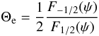 (1)where
Fν(ψ) are the Fermi-Dirac
integrals
(1)where
Fν(ψ) are the Fermi-Dirac
integrals 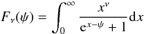 (2)and ψ
is the so-called degeneracy parameter. For ψ → ∞ the electrons are fully
degenerate, whereas for ψ → −∞ they are fully non-degenerate. As
ψ goes from −∞ to ∞ Θe goes from 1 to 0. To obtain
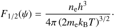
ψ we tabulated
F1/2(ψ) in the
ψ-range of interest and used that it holds that (see e.g. Kippenhahn
& Weigert 1990)
(2)and ψ
is the so-called degeneracy parameter. For ψ → ∞ the electrons are fully
degenerate, whereas for ψ → −∞ they are fully non-degenerate. As
ψ goes from −∞ to ∞ Θe goes from 1 to 0. To obtain
ψ we tabulated
F1/2(ψ) in the
ψ-range of interest and used that it holds that (see e.g. Kippenhahn
& Weigert 1990)
 (3)
(3)
3. Model
A detailed description of the simulation method used in this paper can be found in
Mordasini et al. (2011). Here we only give a brief
outline of its functioning, concentrating on changes to the already existing method. The
following four equations needed to calculate the object structure hold for spherical
symmetric and hydrostatic conditions. They are the standard equations for calculating
stellar structures. The assumption of hydrostatic equilibrium can be justified as the planet
is nearly hydrostatic even in the most critical phase of the radial collapse of the
envelope. This happens at the transition from the attached to the detached phase, where one
finds the kinetic energy of the gas to be many orders of magnitude smaller than the total
energy of the object. 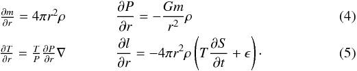 However,
instead of Eq. (5), we use the following
equation
However,
instead of Eq. (5), we use the following
equation  (6)and calculate the
luminostiy as described in Sect. 3.1. The reason why it
is justified to choose ∂l/∂r = 0 is
outlined in Sect. 3.1.1.
(6)and calculate the
luminostiy as described in Sect. 3.1. The reason why it
is justified to choose ∂l/∂r = 0 is
outlined in Sect. 3.1.1.
Equation (5) describes the radial evolution
of the temperature, where the temperature gradient ∇ is defined as
 (7)Following the Schwarzschild
criterion and assuming that the object is either only convective or radiative in a shell, we
set
(7)Following the Schwarzschild
criterion and assuming that the object is either only convective or radiative in a shell, we
set  (8)where
∇ad, the adiabatic temperature gradient, is given directly by the equation of
state (EOS). The radiative temperature gradient ∇rad is defined as
(8)where
∇ad, the adiabatic temperature gradient, is given directly by the equation of
state (EOS). The radiative temperature gradient ∇rad is defined as  (9)In Eq. (9), a denotes the radiation
energy density constant, c the speed of light, κ the
opacity and l = l(r) the luminosity.
Finally, the right part of Eq. (5) yields the
luminosity change per unit radius, where S denotes the entropy per unit
mass. ϵ denotes the thermonuclear energy generation rate per unit mass and
unit time.
(9)In Eq. (9), a denotes the radiation
energy density constant, c the speed of light, κ the
opacity and l = l(r) the luminosity.
Finally, the right part of Eq. (5) yields the
luminosity change per unit radius, where S denotes the entropy per unit
mass. ϵ denotes the thermonuclear energy generation rate per unit mass and
unit time.
3.1. Calculation of the luminosity
Starting from the detached phase1, the model, as
described in Mordasini et al. (2011), uses a
shooting method to find the structure of the object, iterating on the outer radius. As one
needs an surface boundary condition for the luminosity, the following derivation is
chosen: The total energy of the object is  (10)where
u is the internal energy per unit mass. Motivated by the virial theorem
and the fact that our solutions are found assuming a hydrostatic structure, one can
express the total energy of the object as
(10)where
u is the internal energy per unit mass. Motivated by the virial theorem
and the fact that our solutions are found assuming a hydrostatic structure, one can
express the total energy of the object as  (11)The factor
ξ depends on the radial mass distribution inside the object and its
internal energy content2. In order to obtain the
luminosity one can differentiate Eq. (11)
with respect to time which yields
(11)The factor
ξ depends on the radial mass distribution inside the object and its
internal energy content2. In order to obtain the
luminosity one can differentiate Eq. (11)
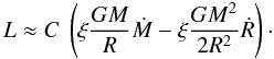
with respect to time which yields 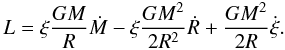 (12)This is only correct,
of course, if we do not have the effect of deuterium burning, which will be included in
the luminosity consideration in the next subsection. As we never know ξ
in advance of the structure calculation at a certain timestep (and thus also
(12)This is only correct,
of course, if we do not have the effect of deuterium burning, which will be included in
the luminosity consideration in the next subsection. As we never know ξ
in advance of the structure calculation at a certain timestep (and thus also
 is unknown), we use the ξ of the previous timestep and approximate
 (13)The correction factor
C accounts for the fact that we excluded the
-term
from our calculation (which we assume to be small, this can be obtained by choosing the
timestep sufficiently short) and that we used ξ from the previous
timestep. An estimate of the correction factor for the next timestep to
t + dt is then found by
(13)The correction factor
C accounts for the fact that we excluded the
-term
from our calculation (which we assume to be small, this can be obtained by choosing the
timestep sufficiently short) and that we used ξ from the previous
timestep. An estimate of the correction factor for the next timestep to
t + dt is then found by
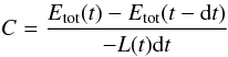 (14)where
the total energies are obtained via the integrals defined in Eq. (10). When considering a hot start, the internal
luminosity Lint (i.e. the luminosity supposed to originate
from within the planet) used to calculate the internal structure of the planet is simply
the luminosity as defined in Eq. (13)
(14)where
the total energies are obtained via the integrals defined in Eq. (10). When considering a hot start, the internal
luminosity Lint (i.e. the luminosity supposed to originate
from within the planet) used to calculate the internal structure of the planet is simply
the luminosity as defined in Eq. (13)
 (15)In the cold start
case we set
(15)In the cold start
case we set 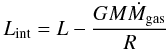 (16)assuming
that the gravitational potential energy released by the gas freely falling onto the planet
is radiated away very efficiently in a shock at the objects surface. This causes the gas
to lose its initially quite high entropy and it is incorporated into the object at a low
specific entropy. One must add, however, that it is still unclear whether objects forming
via the core accretion scenario really form “cold”, as this is depending completely on the
structure of the shock through which the gas is accreted in the runaway accretion phase
(Marley et al. 2007; Stahler et al. 1980). It might be possible that the gas accretion
luminosity should, at least partially, be treated as an internal energy source (commonly
denoted as a “warm start”), i.e. the gas is accreted with a higher specific entropy.
Motivated by the fact that the shock structure and thus the initial entropy of the freshly
accreted gas is not really understood, the post-formation evolution of planets or objects
with initial conditions which lie in the warm start regime were studied recently (Spiegel
& Burrows 2012).
(16)assuming
that the gravitational potential energy released by the gas freely falling onto the planet
is radiated away very efficiently in a shock at the objects surface. This causes the gas
to lose its initially quite high entropy and it is incorporated into the object at a low
specific entropy. One must add, however, that it is still unclear whether objects forming
via the core accretion scenario really form “cold”, as this is depending completely on the
structure of the shock through which the gas is accreted in the runaway accretion phase
(Marley et al. 2007; Stahler et al. 1980). It might be possible that the gas accretion
luminosity should, at least partially, be treated as an internal energy source (commonly
denoted as a “warm start”), i.e. the gas is accreted with a higher specific entropy.
Motivated by the fact that the shock structure and thus the initial entropy of the freshly
accreted gas is not really understood, the post-formation evolution of planets or objects
with initial conditions which lie in the warm start regime were studied recently (Spiegel
& Burrows 2012).
3.1.1. Further simplifications
As one finds the objects to be fully convective in the detached and post-formation evolution phase (except for a thin radiative layer at the outer boundary) we do not calculate the radial structure of the luminosity, as it is not necessary. The radial structure of the luminosity only enters the objects structure calculation via Eq. (5) and only if the radial shells under consideration are radiative (see Eq. (8)). As the objects are basically fully convective, we set dl/dr = 0 (for simplicity), which is not affecting the simulation. Furthermore it has the advantage to also cover the objects evolution in the attached phase, were the main luminosity is due to the solid accretion of the core, thus the luminosity is approximately constant in the gaseous envelope. As shown in Mordasini et al. (2011) the calculation of the structure as explained here leads to evolutionary sequences which are in excellent agreement with the conventional entropy method (see e.g. Burrows et al. 1997; Burrows et al. 2001; and Chabrier & Baraffe 2000). However, a possible caveat might be that we assume the objects to have very effective, large scale convection (i.e. the radiative losses of rising convective blobs are small compared to the energy they transport). This is equal to treating the objects as adiabatic in the convective regions. This, however, must not necessarily be the case (Leconte & Chabrier 2012), given that less effective convection is superadiabatic.
3.2. Adopting the calculation of the correction factor C to deuterium burning
As outlined in the previous section, the boundary luminosity
Lint needed for the structure calculation of the objects can
be approximated by using the virial theorem. In this method, however, the luminosity
contribution of deuterium burning cannot be included directly. To overcome this problem we
utilized the simplification of using the deuterium burning luminosity
LD calculated at the previous timestep, i.e. at
t − dt, and set (for the cold start):
 (17)The error of this
approximation, similarly to the error we make for the approximation of the correction
factor C, gets smaller the smaller we choose the timesteps. In order to
get the correct value of the correction factor C one has to take into
account that the total energy definition in Eq. (10) does not include any term considering the deuterium fusion process. Thus, we
set
(17)The error of this
approximation, similarly to the error we make for the approximation of the correction
factor C, gets smaller the smaller we choose the timesteps. In order to
get the correct value of the correction factor C one has to take into
account that the total energy definition in Eq. (10) does not include any term considering the deuterium fusion process. Thus, we
set  (18)in
order to correct for this. The fact that
LD(t − dt) appears here
instead of LD(t) comes from the just
mentioned problem that we cannot “predict” the deuterium burning luminosity with the
virial theorem ansatz and thus use LD from the previous
timestep. C is thus still the ratio of the actual difference of potential
and internal energy and the estimated energy radiated away due to contraction, cooling and
accretion processes in the timestep of length dt.
(18)in
order to correct for this. The fact that
LD(t − dt) appears here
instead of LD(t) comes from the just
mentioned problem that we cannot “predict” the deuterium burning luminosity with the
virial theorem ansatz and thus use LD from the previous
timestep. C is thus still the ratio of the actual difference of potential
and internal energy and the estimated energy radiated away due to contraction, cooling and
accretion processes in the timestep of length dt.
3.3. Calculation of the deuterium abundance
In order to calculate the decrease of the deuterium abundance we assumed that the deuterium decreases homogeneously in the gaseous envelope. The justification for this is that convective mixing is found to be very effective. Using the mixing length theory and assuming a mixing length equal to the pressure scale height, we found that the convective mixing timescale is always at least 2 or 3 orders of magnitudes smaller than the timescale of deuterium burning.
4. Results of the hot start accreting model and comparison to hot start simulations
In order to test the results we obtain for deuterium burning with our simulation,
especially when varying parameters such as the object’s helium abundance, deuterium
abundance etc., we will compare with the results found by Spiegel et al. (2011, hereafter called SBM11). As SBM11 considered hot
start initial conditions for their evolutionary models we will also use the hot start
condition for the outer boundary condition of the luminosity as described in Sect. 3.1. However, it remains an important difference that in
our model the formation of the objects is taken into account whereas in the model of SBM11
only the evolution of the objects is considered. The other outer boundary conditions for the
evolutionary phase after the formation are  This
are the gray photospheric boundary conditions in the so-called Eddington approximation.
A denotes the albedo of the object. The simulation of SBM11 uses a more
sophisticated atmospheric model, assuming proper non-gray atmospheres. One finds, however,
that the results one obtains with our simple treatment agree well with the results obtained
from the non-gray atmospheric model (Bodenheimer et al. 2000). In Table 1 the definition of our
fiducial model is given. Thus, all other runs of the simulation will only be specified by
the parameters in which they deviate from this fiducial model. In Table 1, a is the distance to the star at
which the planet is supposed to form (migration is disabled),
Σs,0 denotes the initial local surface density of solids,
Tneb and Pneb stand for the
temperature and the pressure in the disk at the location of the planet (the disk evolution
is neglected) and fopa stands for the grain opacity reduction
factor, i.e. the factor by which we assume the grain opacity of the interstellar medium to
be reduced (for further details, see Mordasini et al. 2012). The deuterium number fraction [D/H] is defined as the ratio of the
deuterium and hydrogen atoms. In Table 2 the
definition of the runs carried out in order to compare to SBM11 is given.
This
are the gray photospheric boundary conditions in the so-called Eddington approximation.
A denotes the albedo of the object. The simulation of SBM11 uses a more
sophisticated atmospheric model, assuming proper non-gray atmospheres. One finds, however,
that the results one obtains with our simple treatment agree well with the results obtained
from the non-gray atmospheric model (Bodenheimer et al. 2000). In Table 1 the definition of our
fiducial model is given. Thus, all other runs of the simulation will only be specified by
the parameters in which they deviate from this fiducial model. In Table 1, a is the distance to the star at
which the planet is supposed to form (migration is disabled),
Σs,0 denotes the initial local surface density of solids,
Tneb and Pneb stand for the
temperature and the pressure in the disk at the location of the planet (the disk evolution
is neglected) and fopa stands for the grain opacity reduction
factor, i.e. the factor by which we assume the grain opacity of the interstellar medium to
be reduced (for further details, see Mordasini et al. 2012). The deuterium number fraction [D/H] is defined as the ratio of the
deuterium and hydrogen atoms. In Table 2 the
definition of the runs carried out in order to compare to SBM11 is given.
Fiducial model for the in-situ formation and evolution calculation.
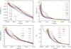 |
Fig. 1 Temporal evolution of the luminosity (upper left), the radius (upper right), the entropy above the core (lower left) and the mass averaged Θe-factor in the envelope (lower right) for hot start objects with masses varying from 10 MJ to 30 MJ using our fiducial model as defined in Table 1. The black dashed line in all plots corresponds to the 13 MJ object. The masses corresponding to the individual lines are indicated in the plot. The horizontal green line in the plot of the radius indicates the position of 1 RJ. |
Hot start comparison runs.
The definition of the metallicity used in Table 2
is the following (we assume scaled solar compositions) ![Mathematical equation: \begin{equation} {\rm [Fe/H]} = {\rm log}_{10}\left(\frac{{\rm Dust-to-gas \ ratio}}{0.04}\right)\cdot \label{equ:metall} \end{equation}](/articles/aa/full_html/2012/11/aa19844-12/aa19844-12-eq87.png) (21)This deviates from the
usual definition of the metallicity as the protosolar mass fraction is found to be 1.49%
(Lodders 2003). In the inner parts of the disk,
however, one should have a higher dust-to-gas ratio: Due to the different orbital velocities
of gas and solids the solids will start to drift inwards such that one finds a dust-to-gas
ratio of approximately 0.04 at 5.2 AU if one considers a solar like star (Rózyczka et al.
2004). The choice of our fiducial model is mainly
motivated by the initial conditions Pollack et al. (1996) chose and represents a model which lies in the regime of conditions one
might expect for an object forming via the core accretion scenario. The reason for taking
the initial deuterium abundance to be 2 × 10⁻⁵ is motivated by Prodanović et al.
(2010), as this is the result they found for the
local interstellar medium. This deuterium abundance of 2 × 10⁻⁵ has more or less
become the standard value when investigating deuterium burning in Brown Dwarfs. It is also
the value used in the fiducial model of SBM11. The choice we made for the initial conditions
of the comparison runs where we vary the helium or the deuterium abundance is based on SBM11
as we want to compare to their results. Our choice for the metallicity (or dust-to-gas
ratio), however, are made due to a different reason. In SBM11 the metallicity has an impact
on the opacity of the object (as a higher metallicity means more molecules and thus a higher
opacity). In our model, however, we assume that all the solids accreted by the objects are
eventually accreted on the core. Thus a higher metallicity (or higher dust-to-gas ratio)
will not change the opacity, but the core mass of the object. For the opacities we assumed a
solar composition and used the opacities of Freedman et al. (2008). The dust-to-gas ratios we chose correspond to the solar case (i.e. [Fe/H] =
0) and to higher metallicities. However, they still lie in the feasible regime (Santos
et al. 2003; Fischer & Valenti 2005). Varying the maximum allowed gas accretion rate is,
of course, also something we cannot compare to SBM11, as they do not consider the formation
process. The motivation for studying different maximum allowed gas accretion rates
(Ṁmax) comes from the fact that different circumstellar disks
will have different properties at different stages during their evolution. The disk
properties such as the viscosity and the surface density determine
Ṁmax (Mordasini et al. 2012). The maximum allowed gas accretion rates we chose also lie in the expected
regime (Mordasini et al. 2012). Finally and of
importance to qualitatively understand the results, is an approximative expression for the
nuclear energy generation rate (Stahler 1988),
(21)This deviates from the
usual definition of the metallicity as the protosolar mass fraction is found to be 1.49%
(Lodders 2003). In the inner parts of the disk,
however, one should have a higher dust-to-gas ratio: Due to the different orbital velocities
of gas and solids the solids will start to drift inwards such that one finds a dust-to-gas
ratio of approximately 0.04 at 5.2 AU if one considers a solar like star (Rózyczka et al.
2004). The choice of our fiducial model is mainly
motivated by the initial conditions Pollack et al. (1996) chose and represents a model which lies in the regime of conditions one
might expect for an object forming via the core accretion scenario. The reason for taking
the initial deuterium abundance to be 2 × 10⁻⁵ is motivated by Prodanović et al.
(2010), as this is the result they found for the
local interstellar medium. This deuterium abundance of 2 × 10⁻⁵ has more or less
become the standard value when investigating deuterium burning in Brown Dwarfs. It is also
the value used in the fiducial model of SBM11. The choice we made for the initial conditions
of the comparison runs where we vary the helium or the deuterium abundance is based on SBM11
as we want to compare to their results. Our choice for the metallicity (or dust-to-gas
ratio), however, are made due to a different reason. In SBM11 the metallicity has an impact
on the opacity of the object (as a higher metallicity means more molecules and thus a higher
opacity). In our model, however, we assume that all the solids accreted by the objects are
eventually accreted on the core. Thus a higher metallicity (or higher dust-to-gas ratio)
will not change the opacity, but the core mass of the object. For the opacities we assumed a
solar composition and used the opacities of Freedman et al. (2008). The dust-to-gas ratios we chose correspond to the solar case (i.e. [Fe/H] =
0) and to higher metallicities. However, they still lie in the feasible regime (Santos
et al. 2003; Fischer & Valenti 2005). Varying the maximum allowed gas accretion rate is,
of course, also something we cannot compare to SBM11, as they do not consider the formation
process. The motivation for studying different maximum allowed gas accretion rates
(Ṁmax) comes from the fact that different circumstellar disks
will have different properties at different stages during their evolution. The disk
properties such as the viscosity and the surface density determine
Ṁmax (Mordasini et al. 2012). The maximum allowed gas accretion rates we chose also lie in the expected
regime (Mordasini et al. 2012). Finally and of
importance to qualitatively understand the results, is an approximative expression for the
nuclear energy generation rate (Stahler 1988),
![Mathematical equation: \begin{equation} \label{equ:stahler} \epsilon \propto {\rm [D/H]} \ \rho \ T^{11.8} \end{equation}](/articles/aa/full_html/2012/11/aa19844-12/aa19844-12-eq89.png) (22)and the
following equation, which approximates the central temperature (see, e. g., Kippenhahn
& Weigert 1990):
(22)and the
following equation, which approximates the central temperature (see, e. g., Kippenhahn
& Weigert 1990):  (23)This equation is obtained
from the equation of hydrostatic equilibrium using the EOS of an ideal gas. We found that
this expression approximates the qualitative behavior of the central temperature quite well
in terms of predicting where it will increase during the phase of collapse and runaway
accretion. However, an important caveat of this approximation is that it assumes an ideal
gas. This is not true as the objects will become more and more degenerate as they contract
and their mass increases (see Sect. 5.2 and Appendix
B).
(23)This equation is obtained
from the equation of hydrostatic equilibrium using the EOS of an ideal gas. We found that
this expression approximates the qualitative behavior of the central temperature quite well
in terms of predicting where it will increase during the phase of collapse and runaway
accretion. However, an important caveat of this approximation is that it assumes an ideal
gas. This is not true as the objects will become more and more degenerate as they contract
and their mass increases (see Sect. 5.2 and Appendix
B).
4.1. Results of the hot start accreting model: overall behavior
First we study and compare the overall behavior of the objects, forming via hot start core accretion, employing our fiducial model. In Fig. 1 one can see the luminosity, the radius, the specific entropy above the core and the mass averaged degeneracy related Θe factor (see Eq. (1)). We show the evolution starting at 106 years, as the foregoing growth of the solid core to the isolation mass and the subsequent attached phase of the object are equal in the cold start case of the core accretion scenario.
As one can see in the radius plot of Fig. 1, as the planets are still growing in mass via runaway mass accretion, they will also grow in size (after having collapsed due to the transition from the attached to the detached phase) until they have reached their final mass. The end of the mass accretion produces as sharp bend at approximately 3 × 10⁶ years in the radius evolution for the 30 MJ object (and earlier for the lower mass objects) and inverts the radius growth phase into a contraction phase. This is a difference to the cold start model of the core accretion scenario, where one observes a gradual contraction of the planet once it has collapsed when entering the detached phase (see e.g. Mordasini et al. 2011; Marley et al. 2007). This difference is due to the inclusion of accretion luminosity into the internal luminosity. Thus the gas is not accreted onto the already contracting object as in a cold start, but it is accreted injecting all its released gravitational potential energy into the object, which prevents it from contraction. This means that the gas is accreted at high entropy. The radii one finds directly at the end of formation can be regarded as possible initial radii for hot start evolution models if one assumes that the objects have formed according to the core accretion scenario. However, there is one caveat which must be addressed: As the accreted gas first deposits it’s liberated gravitational energy in the upper regions of the object in the runaway accretion phase of a hot start, the simplifiying assumptions made for the luminosity in Sect. 3.1.1 might break down. During a “hot” accretion radiative zones well inside the object could develop (see e.g. Mercer-Smith et al. 1984), so that our assumption that dl/dr = 0 becomes invalid in these regions. Thus by forcing the object to have an adiabatic structure our results could depart quite significantly from the correct values in this phase. However, as the Kelvin-Helmholtz timescale of an object at the end of formation is very short the objects would quickly forget about their thermodynamic state directly after the formation, evolving back on the correct evolutionary track (provided that the latter is not characterized by a much lower entropy). Thus one should be cautious when interpreting our results directly after formation as initial conditions for a hot start evolutionary model.
Looking at the specific entropy above the core in Fig. 1 one can see how the most massive object (30 MJ) reaches a specific entropy as high as 14.5 kB/Baryon due to the accretion of high entropy material (which is characteristic for a hot start). We note here as well that these values found for the specific entropy at the end of formation might be realistic initial values for evolution calculations if one assumes that the objects have formed via core accretion. However one should keep in mind the caveat outlined above. As the objects are fully convective in their interior (and thus have an adiabatic temperature gradient) the specific entropy is constant throughout the envelope. Again one sees that also the decrease of the entropy is partially stabilized by deuterium burning.
In the Θe plot of Fig. 1 one sees how the degeneracy related factor Θe (see Eq. (1)) evolves. For this plot Θe was mass averaged in the gaseous envelope. As one can see the envelope starts fully non-degenerate (Θe = 1) and reaches a first minimum at approximately Θe = 0.7. Instead of starting at 106 years as all other plots of Fig. 1, the Θe plot starts at 105 years in oder to show the initial value of Θe = 1. After having reached a value of 0.7, Θe then starts to increase again at the beginning of the runaway phase and then drops down to 0.6 at the moment where the objects envelope collapses (at ≈ 106 years). One can see that deuterium burning will partially stabilize Θe as well. After this stabilization phase, however, Θe will start do decrease stronger again, approaching small values between 0 and 0.1 at the end of the simulation, corresponding to stronger degeneracy.
4.1.1. Comparison of the stabilization radii to the results of Burrows et al. (1997)
As the SBM11 hot start calculations (to which we compare our work in the next section) are based on the model of Burrows et al. (1997), it seemed worthwhile to compare to those results, especially as the data of the Burrows et al. (1997) is available online. In Fig. 2 one can see the radius evolution obtained by Burrows et al. (1997) (dashed green lines) and our own results (red solid lines). The results of Burrows et al. (1997) have been shifted in time in order to make the phases of deuterium burning coincide. This is justified as the Burrows et al. (1997) results do not consider the formation of the object, thus the definition of t = 0 is not equal. As one can see in Fig. 2, the radius at which the partial stabilization of the objects occurs is the same in both models and also the subsequent radial evolutions are nearly equal. This again underlines the reliability of our model assumptions, i.e. the way how we calculate the luminosity and the way how deuterium burning was included into the simulation.
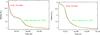 |
Fig. 2 Radial evolution of deuterium burning objects (hot start accretion). The solid red lines show our own results, whereas the dashed green lines show the results of Burrows et al. (1997). As the t = 0 definition is not the same, the Burrows et al. (1997) results where shifted in time in order to make the phases of deuterium burning coincide. The mass of the objects is indicated in the plots. |
4.1.2. Comparison to the SBM11 results
Comparison with SBM11 (SBM11 also assumed a helium mass fraction of 0.25, along with a deuterium number fraction with respect to hydrogen of 2 × 10⁻⁵ as their fiducial model) shows that the radii at which the planets become partially supported against contraction by deuterium burning roughly coincide with our results. A 20 MJ object will be in this phase at a radius between 2 and 2.5 Jupiter radii in the SBM11 results, which agrees with our findings. For the lower mass objects in the 14 to 15 MJ range this phase lies around 1.5 Jupiter radii which is also true for our results.
Furthermore, when looking at the evolution of the ratio LD/Ltot we find that for a 13 MJ object it peaks at approximately 0.5 which is the same result SBM11 obtain. Also, we and SBM11 both find that for M ≳ 14 MJ the peak of LD/Ltot is above 0.8, reaching more than 0.9 for the heavier objects ≳ 20 MJ. The results for LD/Ltot for objects below 12 MJ are also similar to the SBM11 results, the only deviation is observed for the 12 MJ object, where our peak value for LD/Ltot is twice as high. One must note, however, that LD/Ltot is a very steep function of the mass in this range, thus slight differences in the models might be seen quite strongly.
Also, when looking at the luminosities at which the objects are partially stabilized due to deuterium burning we find a very good agreement between our results and those of SBM11.
In our model and in the model of SBM11 the metallicity enters in two different ways: it sets the opacity in the SBM11 case and the core mass in our case. As both SBM11 and we ourselves find that the metallicity has a significant influence on the deuterium burning process (see Sect. 4.2), it is rather a coincidence that we straightaway found the metallicity for our fiducial model such that it yields approximately the same deuterium burning behavior as in the SBM11 case. Thus even though they also assumed a solar metallicity in their fiducial model it was per se not clear that we would get a good agreement. It shows, however, that once one has found this metallicity value which seems to correct for the effect of the different implications of the metallicities in both models, the results seem to be approximately the same in all considered quantities.
4.2. Parameter study
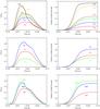 |
Fig. 3 Left column: the ratio LD/Ltot. Right column: the depletion of deuterium. The first row shows our results for different helium abundances, the second row shows the influence of different deuterium abundances and the last row shows different dust-to-gas ratios (as defined in Table 2). The mass of all objects is 13 MJ (hot start). The run names corresponding to the individual lines are indicated in the plot. |
In their paper, SBM11 tested how the deuterium burning process is influenced when parameters such as the hydrogen abundance, the deuterium abundance and the metallicity are varied. We also carry out this parameter study to further test our own simulation, before we proceed to the study of the cold start results of objects forming by core accretion in Section 5. In the upper left and right panel of Fig. 3 one can see the LD/Ltot evolution and the deuterium depletion for the runs with different helium abundances (Y22-Y30) for a 13 MJ object.
The bumpy pattern in some LD/Ltot plots is due to the interpolation of the opacities in the tables of Freedman et al. (2008) and thus a numerical artifact.
Concerning the height of the LD/Ltot peaks we again find a very good agreement with the results of SBM11. We do, however, also observe that our objects burn 10–50% more deuterium as they sustain a high burning rate over a longer period of time. Overall, we thus confirm the fact that a higher helium abundance yields a stronger deuterium burning process, due to the increased central density of the objects (see Eq. (22))3. The results of the runs with different deuterium abundances (D1, D2 and D4) are shown in middle row of Fig. 3. Again, we find a very good agreement when comparing to the peak value of LD/Ltot of the Spiegel et al. (2011) results. Furthermore, we again find the already mentioned fact that our objects burn more deuterium than in the SBM11 case. A possible reason for this could be the use of different opacities. Higher opacities enable the objects to keep high central temperatures over a longer period of time (the so-called blanket effect). Furthermore SBM11 use a proper atmospheric model while we use gray photospheric boundary conditions. As the deuterium burning rate is depending on the temperature very strongly (see Eq. (22)) this can sustain the burning rate over a longer period of time as well. We conclude that we are in a good agreement with the results by SBM11 but out objects burn up to 50% more deuterium. Finally we consider the runs with varied dust-to-gas ratio (i.e. varied metallicity) and with varied maximum allowed gas accretion rates, which we cannot compare to the SBM11 results, as they do not consider the formation process or the presence of solid cores. It is worthwhile to study the impact of these parameters nonetheless. In the lower row of Fig. 3 one can see the results obtained for the LD/Ltot evolution and for the deuterium depletion for runs with different dust to gas ratios fpg1, fpg2 and fpg3, corresponding to dust-to-gas ratios of 0.04, 0.09 and 0.12, respectively. The considered dust-to-gas ratios have a significant influence on the deuterium burning behavior. The higher it is, the higher the nuclear burning luminosity compared to the total luminosity and the more deuterium is burned. One can, in principle, imagine at least two reasons for this behavior.
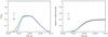 |
Fig. 4 Left panel: the ratio LD/Ltot as a function of time. Right panel: the depletion of deuterium for the runs with different maximum allowed mass accretion rates (as defined in Table 2). The mass of the objects is 13 MJ (hot start). The run names corresponding to the individual lines are indicated in the plot. |
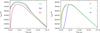 |
Fig. 5 Central temperature for the different dust-to-gas ratio runs (left plot) and for the different maximum allowed gas accretion runs (right plot) (hot start). |
One reason is that a higher dust-to-gas ratio will lead to a higher solid surface density in the disk, which will in turn lead to a higher solid accretion rate. A higher solid accretion rate also means a higher core luminosity, which might influence the objects structure as the core accretion luminosity is included into the structure calculation. This is motivated by the assumption of our model that the solids impacting the object get destroyed and the debris then sinks to the core, following the so-called sinking approximation (Pollack et al. 1996). Thus one would expect the central temperature to be higher, which has a large influence on deuterium burning, as the nuclear energy generation rate is highly dependent on the temperature (see Eq. (22)).
The other possible reason is due to the fact that we assume that all solids accreted by
the object eventually get incorporated in the core, leading to a higher core mass. A
higher core mass will, even though the core is also growing in size as it grows in mass,
result in a higher gravitational acceleration on top of the core. In order to remain in
hydrostatic equilibrium one thus needs a higher pressure gradient, i. e. a higher
temperature gradient, as the temperature gradient in a convective layer (which the central
gas layer surely is) is 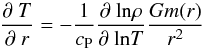 (24)which
is proportional to the gravitational acceleration. This means that a higher temperature
gradient might lead to a higher central temperature, if it dominates over the fact that
the gas cannot reach as deep within the object as it could with a lighter core (as objects
with a higher core mass are found to have a smaller total radius and a larger core
radius). If it does, this would create a higher deuterium burning rate.
(24)which
is proportional to the gravitational acceleration. This means that a higher temperature
gradient might lead to a higher central temperature, if it dominates over the fact that
the gas cannot reach as deep within the object as it could with a lighter core (as objects
with a higher core mass are found to have a smaller total radius and a larger core
radius). If it does, this would create a higher deuterium burning rate.
We were able to identify that it is rather the increased core mass than the additional core accretion luminosity which affects the deuterium burning process in the following way: in Fig. 4, one can see the LD/Ltot evolution and the deuterium depletion for the runs with a different maximum gas accretion rate (A1–A3). As one can see, the object with the lowest maximum mass accretion rate reaches the the peak value the latest, as it needs a longer time to form. However, all three runs have the same peak value of LD/Ltot, and the same subsequent evolution of LD/Ltot after having reached the peak value. One can also see that all three runs burn approximately the same amount of deuterium. The remaining slight variations in the A1–A3 runs for the peak values of LD/Ltot and the deuterium depletion are mainly due to a simulation artifact: as we cannot switch off the accretion instantaneously (in order to remain numerically stable) it is difficult to exactly reach the desired total mass. The deuterium burning rate depends on the objects density (see Eq. (22)) and thus one can see that a slightly different final mass will have an impact.
In conclusion we see that the amount of deuterium burned and the strength of deuterium burning is independent of the luminosity due to gas accretion, which is included in the internal luminosity in the hot start case (see Eq. (15)). We have furthermore found that the contribution of the solid accretion luminosity to the total accretion luminosity is very small in the phase of runaway gas accretion. This makes it very unlikely that the different solid accretion luminosities in the runs with different dust-to-gas ratios (“fpg”-runs) have a strong impact on the deuterium burning process. The luminosity due to gas accretion is much stronger, but apparently has very little effect on deuterium burning. It rather seems to be the presence of the core itself which influences deuterium burning via Eq. (24).
In order to further show this, we plot in Fig. 5 the central temperature for the different dust-to-gas ratios and for the different maximum gas accretion rates. One clearly sees that for the runs with different dust-to-gas ratios, the central temperature is always higher for the runs with higher dust-to-gas ratio, which persists until the end of the simulation at 1010 years. The runs with different maximum gas accretion rate, however, reach approximately the same central temperature at the end of formation and their subsequent central temperature is the same. The core masses for the three runs “fpg1”, “fpg2” and “fpg3” are 35.2 M ⊕ , 77.5 M ⊕ and 101.5 M ⊕ , respectively. For the three runs “A1”, “A2” and “A3” the core masses are 39.1 M ⊕ , 35.2 M ⊕ and 31.2 M ⊕ .
Parameter study for cold start simulations.
5. Cold start scenario
In this main section, we consider the formation of objects forming via the core accretion scenario using the cold start assumption, which means that all gravitational energy liberated at the accretion shock is radiated away, not contributing to the internal luminosity (see Eq. (16)). This is equivalent to the accretion of low entropy material. We stress again, however, that it is still an open question whether the total accretional luminosity is radiated away at the shock (Marley et al. 2007; Stahler et al. 1980). A cold start is the standart scenario for the formation via core accretion with a gradual accretion of matter. The typical timescale for the runaway gas accretion phase during the formation of a 13 MJ object is approximately 4 × 10⁵ years if one considers a Ṁmax of 10-2M ⊕ /yr (almost the complete mass of the object is accreted in the runaway phase). This is quite long compared to the typical formation timescale of direct collapse models, which is approximately equal to the orbital timescale and of the order of 102–103 years in the distances feasible for a direct collapse to occur (adirect ≥ 50 AU for 10 MJ) (Janson et al. 2011). It is, however, unclear if a clump at final mass forms in the direct collapse model or whether it would accrete gas as well. For our fiducial model, we will use the parameters specified in Table 1. In Sect. 5.1, we study the general behavior of objects forming with a cold start. In Sect. 5.2 we investigate the minimum mass limit for deuterium burning. In order to do so we vary the parameters of the model and carried out the runs given in Table 3.
5.1. Overall behavior
In order to understand the implications of deuterium burning on the evolution of objects forming via core accretion and a radiatively effective shock we first describe the qualitative behavior studying the formation and subsequent evolution of a 16 MJ object. In order to get an understanding for the changes deuterium burning introduces to the internal structure we also consider the artificial cases where either deuterium burning is disabled, or where the deuterium abundance is kept constant. Figure 6 shows the evolution of the object’s luminosity, it’s radius and it’s central and surface temperature for the three cases (deuterium burning, no deuterium burning, constant deuterium abundance). Differences in the evolution can only be seen after the object’s formation is completed, as marked by the end of runaway gas accretion which produces the sharp decrease in the luminosity at approximately 1.3 × 10⁶ years. This is due to the disappearance of the accretion luminosity. It is clear, however, that the phases preceding the gas runaway accretion cannot be important for deuterium burning, as the temperatures as well as the densities in the gaseous layers are far too low.
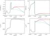 |
Fig. 6 Formation and subsequent evolution of a 16 MJ object forming via core accretion with a radiatively efficient shock (cold start). The four panels show the temporal evolution of the total luminosity (internal + shock) (upper left), the radius (upper right), the central temperature (lower left) and the surface temperature (lower right). The dotted blue line shows the results obtained for the fiducial model as specified in Table 1. For the solid red line, the deuterium abundance was kept constant, while for the dashed green line, deuterium burning was disabled. |
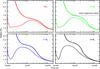 |
Fig. 7 Radius as a function of time for objects forming via the hot start ansatz (solid line) or the cold start ansatz (dashed line). The mass of the objects is indicated in each panel. In the upper right panel (16 MJ) the gray lines show the results obtained for a constant deuterium abundance. |
5.1.1. Luminosity
Concentrating on the panel with the luminosity in Fig. 6, we see that after the formation of the object, the deuterium burning will cause the object to behave quite differently. We first note that deuterium burning produces an additional, rather flat peak in luminosity at approximately 107 years where the luminosity is an order of magnitude higher than in the case with deuterium burning disabled. We also see that for objects where the deuterium abundance is kept constant, the objects will reach a (hypothetical) deuterium burning main sequence, where the object’s luminosity is generated by deuterium burning only. This is what one would naively expect when keeping the deuterium abundance constant.
5.1.2. Radius
Comparing to the hot start scenario (see Fig. 1), a clearly different behavior can be seen for the evolution of the radius. Instead of stabilizing the objects against further contraction as in the hot start case, the onset of deuterium burning is so strong that the object is inflated from 1.2 to approximately 1.7 RJ for the nominal case. This suggests that a large part of the deuterium burning luminosity is converted into gravitational potential energy in that phase, which corresponds to a LD/Lint ratio (much) larger than 1 (we will discuss this later). Thus, instead of contracting and cooling at high temperatures and gradually burning deuterium already at quite large radii as in the hot start case, a cold start yields a more abrupt start of deuterium burning. This is due to the effect that the mass is accreted at low entropy onto an object with high density, due to the collapse from the attached to the detached phase. Thus the objects have then much higher burning rates as the objects are already very dense when they reach the temperature needed for deuterium burning (see Eq. (22)). The expansion process will be discussed in more detail below.
5.1.3. Temperatures
Finally, one can see that deuterium burning also produces a flat peak in the central and in the surface temperature when compared to the case without deuterium burning. The case where the deuterium abundance was set constant yields a main sequence-like behavior again.
5.1.4. Expansion
In order to understand the expansion we compare the radii to which the objects expand in the cold start scenario with the radii at which the objects get partially stabilized against contraction in the hot start case. A comparison like this seems sensible as it is well known that nuclear fusion processes in stars, such as hydrogen burning, have a thermostatic behavior (also known as the pressure temperature thermostat or stellar thermostat) (see, e.g. Palla et al. 2002). This can also be seen very clearly in the runs with constant deuterium abundance, as the objects, driven by deuterium burning, attain a stable state in the hypothetical deuterium main sequence. Given the thermostatic nature of deuterium burning, we expect the cold start objects to expand to approximately the same radii found for the hot start objects in the phase where they get partially stabilized. More precisely, as the objects in the hot start case are unable to completely stabilize themselves against further contraction (as LD/Ltot is always smaller than 1) we expect that the cold start objects will not be able to expand to the same radii as the “quasi-stabilization”-radii of the hot start objects, but to a somewhat smaller radius. The reason for LD/Ltot < 1 in the hot start case, as well as for the somewhat smaller expansion radius in the cold start case is the decreasing deuterium abundance inside the objects. When looking at Fig. 7 we can see this behavior: the cold start objects expand to radii somewhat smaller than the radii at which the hot start objects are partially stabilized. When this radius increases for the hot start objects (i.e. for higher masses) it also does so for the cold start objects. For the 16 MJ object in Fig. 7, we have also plotted the radius evolution for hot and cold start with deuterium abundances held artificially constant. As one can see, they both get stabilized at the same radius (which we call “main sequence radius” in the plot). The hot start object contracts to this radius from above, whereas the cold start object is at a smaller radius when deuterium fusion ignites and must thus expand to the main sequence radius. One can observe that the main sequence radius approximately coincides with the “quasi-stabilization” radius of the hot start object. Thus, the consideration of the in principle unphysical (artificially held constant deuterium abundance) main sequence radius and the thermostatic nature of nuclear fusion processes help to understand not only the stabilization behavior of the hot start objects, but also the expansion behavior of the cold start objects.
5.1.5. Evolutionary sequences for objects formed by core accretion, assuming a cold start
Similar to Fig. 1 for the hot start case we also show the temporal evolution of the luminosity, the surface temperature, the radius, the gravitational acceleration at the surface, the specific entropy and the mass averaged degeneracy parameter Θe for the cold start case in Fig. 8. Except for Θe, the evolution is shown starting at 106 years, i.e. shortly before the final mass is reached, and therefore shows the final stages of the object’s formation in the runaway accretion phase. The time axis of Θe starts at 105 years in order to see that the envelope indeed was fully non-degenerate in the beginning.
The luminosity shown in the plot is the total luminosity, i.e. the sum of the internal luminosity and the accretion luminosity, as this is the luminosity which would be seen by an observer. The sharp drop in luminosity (from approximately 0.1 L⊙ for the 23 MJ object) marks the end of runaway gas accretion and thus the end of the formation process. One can see that for the lower masses up to 13 MJ there is no additional bump in the luminosity. Instead it decreases monotonously. For the objects of higher masses, however, the luminosity does not decrease monotonously but has an additional bump due to deuterium burning. For almost all masses shown in the plot the maximum luminosity due to deuterium burning is reached far after the end of formation. For the 23 MJ object this is not the case: the luminosity does not increase strongly anymore after the end of formation and indeed one finds that the 23 MJ object burns almost all of it’s deuterium during the formation phase (this is discussed in more detail in Sect. 5.1.6). One can also observe that the higher the mass of the object the higher is the bump in luminosity.
A similar behavior is found for the surface temperature: The objects of masses up to 13 MJ do not exhibit an additional bump due to deuterium burning. All objects with masses above, however, do. The peak value of the increased surface temperature is increasing with mass. Directly after formation the 23 MJ object is over 1000 K hotter than the 13 MJ object. As well as in the luminosity case the peak value of the deuterium burning induced temperature bump is reached later for the lower mass objects. The time difference between the 23 MJ object and the 14 MJ object is approximately 5 × 10⁷ years.
Everything which was said about the luminosity and the surface temperature also applies for the radius, the entropy and the degeneracy factor Θe. Deuterium burning introduces an additional bump in the temporal evolution of these quantities for masses above 13 MJ. The peak value of these bumps will be reached later for the less massive objects and the peak value will be smaller.
For the surface gravity it also holds that no deuterium burning caused effect can be seen for masses up to 13 MJ. For the more massive objects deuterium burning produces a dip, rather than a bump, as the gravitational acceleration is proportional to R-2, where R is the radius of the object.
Finally it is important to note that the fact that no additional bump or dip is seen for masses up to 13 MJ does not necessarily mean that these objects do not burn deuterium at all. As we will discuss in the following sections, objects with masses around 13 MJ already burn significant amounts of their deuterium. The effect of deuterium burning does not introduce an additional bump or dip but it slows down the monotonous decrease (or increase for log (g)) of the discussed quantities.
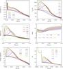 |
Fig. 8 Temporal evolution (for cold start objects) of the luminosity as seen by an observer, i.e. including the accretion luminosity (first row, left), the surface temperature (first row, right), the radius (second row, left), the gravitational acceleration at the surface (second row, right), the specific entropy above the core (third row, left) and the degeneracy related factor Θe (third row, right) for objects with masses varying from 10 MJ to 23 MJ using our fiducial model as defined in Table 1. The black dashed line in all plots corresponds to the 13 MJ object. The horizontal green line in the plot of the radius indicates the position of 1 RJ. The masses corresponding to the lines are indicated in the plot. |
5.1.6. Implications of the gas runaway accretion phase
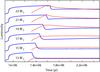 |
Fig. 9 Evolution of the luminosities of cold start objects with masses as indicated in the plot. The blue solid lines show the total luminosities of the objects (i.e. the luminosity an observer would see), whereas the dashed red lines denote the luminosity due to deuterium burning only. The luminosities for the different masses have been separated in the y-axis by an arbitrary offset for better visibility. Up to approximately 1.3 × 10⁶ years, where the gas runaway accretion ends for the 13 MJ object, all objects have the same luminosity. |
We now concentrate on the behavior of deuterium burning and how it is influenced by the mode of formation of the objects, which is a core accretion formation with a radiatively efficient shock (cold start). As we have already seen, a major difference comes from the fact that cold start objects start deuterium burning at a much smaller radius than in the hot start case. Then they expand approximately to the radius they attain in a hypothetical deuterium main sequence, due to the thermostatic nature of deuterium burning. In Fig. 9 one sees the evolution of the total luminosity Ltot and of the luminosity due to deuterium burning (LD) for objects of different masses. When studying the plot one can notice that the end of gas runaway accretion (marked by the steep decrease in the total luminosity of the objects) causes a bend in LD for all masses, which is clearer for the lower masses. For the lower masses up to 17 MJ, the growth of LD, which is strongly increasing in the gas runaway phase, is brought to a halt and remains approximately constant. For the heavier masses, LD will decrease after the end of the gas runaway accretion. Furthermore we observe that for the higher masses (≈ 23 MJ), LD reaches a peak still during the phase of gas runaway accretion, then decreases slightly before showing the bend at the end of gas runaway accretion, after which it decreases even faster. This behavior can be explained with the Eqs. (22) and (23). After the object has collapsed at the transition from the attached to the detached phase, it is not yet massive enough to burn deuterium. Furthermore, due to the cold start assumption the (major) part of the planets mass is then added onto the planet at low entropy, meaning that it grows in mass while contracting even further. As the central temperature is proportional to M/R (Eq. (23)) and the deuterium burning rate is depends on the temperature very strongly and linearly on the density (Eq. (22)), this process of adding mass on the object will cause the observed increase of LD in the phase of runaway mass accretion. The sharp bend in LD at the end of gas runaway accretion nicely shows the dependence of LD on the process of runaway accretion (as the object has stopped mass accretion LD ceases it’s strong increase). For the objects of heavier masses, which exhibit a peak of deuterium burning inside the phase of gas runaway accretion, another effect becomes important. As one can see in Eq. (22), the fusion rate of deuterium burning is proportional to the deuterium abundance. Indeed we find that those objects burn most of their deuterium already during their formation phase (as higher masses mean a higher central temperature and thus a higher deuterium burning rate). Thus, at some point, LD will not increase further even though the central temperature is still rising, as the effect of the decreasing deuterium abundance becomes stronger. The reason for the following modest decrease of LD in the runaway phase is that the still increasing central temperature (due to Eq. (23)) will partially counterbalance the impact of the decreasing deuterium abundance.
Finally, as already said above, the objects expand due to deuterium burning. Thus LD must overshoot the intrinsic luminosity (to which it contributes) in the expansion phase.
5.2. Sensitivity of the minimum mass limit of deuterium burning
Similar to the paper of SBM11, we will investigate the implication of certain quantities on the process of deuterium burning, namely in terms of how they affect the minimum mass limit for deuterium fusion. In order to do so, we assume a core accretion formation, use the cold start assumption and consider the runs as specified in Table 3. As SBM11 pointed out, no exact border can be drawn between deuterium burning and non-deuterium burning objects, as the amount of burned deuterium varies smoothly as a function of mass instead of exhibiting a sharp transition. In this paper, if an object decreases it’s initial deuterium abundance by more than 50%, we will call it for simplicity a deuterium burning object and objects below this border will be called non-deuterium burning objects. The mass at which this transition happens will be called M50. One should however bear in mind that this choice of the position of the border is partially arbitrary, even though 50% seems to be a sensible choice, as it is in the middle of the two cases of (almost) no deuterium burning and complete deuterium combustion. This illustrates the problem which arises if one persists on the rigorous distinction of planets and Brown Dwarfs in the mass regime considered henceforth.
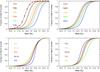 |
Fig. 10 Fraction of the initial deuterium burned as a function of mass until the end of the simulation (1010 years) for cold start objects. Top left: results for different helium fractions. Top right: results with different dust-to-gas ratios (or metallicities). Bottom left: results for different maximum gas accretion rates. Bottom right: results for different deuterium abundances. The uppermost run names in the plots correspond to the leftmost curves, the next lower run names correspond to the second leftmost curves etc. For the Y30 run in the upper left panel the positions of the individual mass runs are indicated with filled brown circles. For the sake of clarity we omitted plotting the individual mass run positions for all other runs. Instead a spline function was plotted through the individual mass run positions. |
In Fig. 10 one can see the results we obtain for the runs in Table 3. The fraction of the initial deuterium which has been burned until the end of the simulation (1010 years) is plotted against the total mass of the objects. As one can see, the transition from objects which burn no deuterium to objects which burn all their deuterium has a width of approximately 5 MJ and takes place roughly between 10 and 15 MJ.
As one can see in Fig. 10, the largest impact on changing M50 has the variation of the helium abundance. It must be noted, however, that a helium abundance as low as 0.22 is rather improbable, as the helium fraction due to the primordial nucleosynthesis was approximately 0.25 (Spergel et al. 2007) and has, since then, increased in time due to hydrogen fusion in stars. The top and bottom right panel of Fig. 10 show that a variation of the metallicity, as well as the variation of the deuterium abundance, will shift the place of the transition region between deuterium burning and non deuterium burning objects.
When considering the maximum mass accretion rate Ṁmax (bottom
left panel) we find that, opposite to the results obtained for the hot start case,
Ṁmax now also has an impact on the process of deuterium
burning. The reason for this is the following: The objects collapse at the transition from
the attached to the detached phase (as can be seen at approximately 106 years
in the upper right plot in Fig. 6 showing the radius
evolution). After this collapse the objects will contract further while they accrete most
of their mass during the runaway accretion process. This is in contrast to the hot start
case, where the objects expand again during the runaway accretion. It is clear that the
higher the maximum allowed mass accretion rate, the shorter is the time the object will
have to contract during the runaway accretion process. The consequence of this is the
following: At higher Ṁmax, the gas accretes onto a larger
object, which means that the free fall velocity of the gas at the moment it reaches the
surface of the object will be smaller, as the free fall velocity for the infalling matter
is  (25)Mdenotes
the mass of the object, R is the radius of the object and
G the gravitational constant. The lower free fall velocity would result
in a smaller accretion luminosity if Ṁmax was constant (cf.
Bodenheimer et al. 2000)
(25)Mdenotes
the mass of the object, R is the radius of the object and
G the gravitational constant. The lower free fall velocity would result
in a smaller accretion luminosity if Ṁmax was constant (cf.
Bodenheimer et al. 2000)
 (26)The lower accretion
luminosity per accreted mass unit means that less liberated gravitational potential energy
is radiated away at the shock, or in other words, that matter of higher entropy is
incorporated into the object. This can be understood by the fact that although the object
forms according to a cold start the material is incorporated into the object at larger
radii. Thus it must have a larger specific entropy, just as the initial radius of hot
start simulations is increasing with the chosen initial entropy for fully adiabatic
objects. We find that the accretion of matter with a higher entropy means that the object
will have a higher central temperature, leading to higher deuterium burning rates. The
effect of a higher central temperature due to a higher specific entropy might surprise in
view of the classical result obtained for the central temperature of a self-gravitating
sphere of ideal gas (see Eq. (23)): A
higher specific entropy in fully convective (i.e. adiabatic) objects generally implies a
larger radius (see also Spiegel & Burrows 2012). This, in turn, should cause a lower central temperature (see Eq. (23)). In the cases considered here, however,
partial degeneracy already plays an important role. The fact that the degeneracy becomes
stronger for smaller radii as well as the fact that fully degenrate objects cool as they
shrink (e.g. white dwarfs) underlines that a larger radii due to a higher specific entropy
must not generally imply a smaller central temperature. Also the presence of the core can
cause the envelope to cool. Both arguments are outlined analytically in the
Appendices A and B. In Fig. 11 one can see see how the
central temperature decreases as the entropy decreases in a
7 MJ planet in the post-formation evolutionary phase.
(26)The lower accretion
luminosity per accreted mass unit means that less liberated gravitational potential energy
is radiated away at the shock, or in other words, that matter of higher entropy is
incorporated into the object. This can be understood by the fact that although the object
forms according to a cold start the material is incorporated into the object at larger
radii. Thus it must have a larger specific entropy, just as the initial radius of hot
start simulations is increasing with the chosen initial entropy for fully adiabatic
objects. We find that the accretion of matter with a higher entropy means that the object
will have a higher central temperature, leading to higher deuterium burning rates. The
effect of a higher central temperature due to a higher specific entropy might surprise in
view of the classical result obtained for the central temperature of a self-gravitating
sphere of ideal gas (see Eq. (23)): A
higher specific entropy in fully convective (i.e. adiabatic) objects generally implies a
larger radius (see also Spiegel & Burrows 2012). This, in turn, should cause a lower central temperature (see Eq. (23)). In the cases considered here, however,
partial degeneracy already plays an important role. The fact that the degeneracy becomes
stronger for smaller radii as well as the fact that fully degenrate objects cool as they
shrink (e.g. white dwarfs) underlines that a larger radii due to a higher specific entropy
must not generally imply a smaller central temperature. Also the presence of the core can
cause the envelope to cool. Both arguments are outlined analytically in the
Appendices A and B. In Fig. 11 one can see see how the
central temperature decreases as the entropy decreases in a
7 MJ planet in the post-formation evolutionary phase.
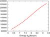 |
Fig. 11 Central temperature of a 7 MJ planet as a function of it’s specific entropy showing the complete post-formation evolutionary phase. |
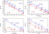 |
Fig. 12 Masses at which 50% of the deuterium has been burned by 1010 years. Upper row, left: varied helium fraction. Right: varied metallicities. Lower row, left: varied maximum gas accretion rates. Right: varied deuterium abundances. The red dashed line shows the fitted functions for the hot start objects (lower line in all plots), while the fits for the cold start objects are plotted in a blue solid line (upper line in all plots). The blue diamonds show the positions of M50 in the cold start runs, while the red semi-filled circles show the positions of M50 for the hot start runs. |
5.2.1. Detailed study of the behavior of M50
Figure 12 shows how
M50 varies due to changes in the helium abundance
Y, the maximum allowed runaway gas accretion
rate Ṁmax, the deuterium abundance [D/H] and the
metallicity [Fe/H] (corresponding to different dust-to-gas ratios). The results obtained
for cold start objects are plotted in blue, while the results obtained for hot start
objects are plotted in red (we varied the fiducial model for the hot start objects in
the same way as we varied it for the cold start objects given in Table 3, but suffixed the run names with an “h” instead of
a “c”). For Y, [D/H] and [Fe/H] the results were fitted to a line using
the least square method: ![Mathematical equation: \begin{align} \nonumber M_{50}/\mj & = m_Y \ Y + b_Y \\ M_{50}/\mj & = m_{\rm [D/H]} \ {\rm [D/H]} + b_{\rm [D/H]}\\ \nonumber M_{50}/\mj & = m_{\rm [Fe/H]} \ {\rm [Fe/H]} + b_{\rm [Fe/H]}. \end{align}](/articles/aa/full_html/2012/11/aa19844-12/aa19844-12-eq139.png) (27)For
Ṁmax (note the logarithmic x-axis in
Fig. 12 for Ṁmax)
the results were fitted to the function
(27)For
Ṁmax (note the logarithmic x-axis in
Fig. 12 for Ṁmax)
the results were fitted to the function
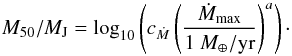 (28)This means that
in a first approximation M50 depends linearly on the helium
abundance Y, the deuterium number fraction [D/H] and the metallicity
[Fe/H]. For Ṁmax and the dust-to-gas ratio (see Eq. (21)), however, there is a logarithmic
dependence.
(28)This means that
in a first approximation M50 depends linearly on the helium
abundance Y, the deuterium number fraction [D/H] and the metallicity
[Fe/H]. For Ṁmax and the dust-to-gas ratio (see Eq. (21)), however, there is a logarithmic
dependence.
The upper right panel of Fig. 10 shows the metallicity dependence of M50. However, instead of labeling the x-axis with “[Fe/H]” it was labeled with “ [Fe/H] loc,gas”. The intention of this is the following: In our model the metallicity sets the dust-to-gas ratio via Eq. (21), which is only valid at approximately 5.2 AU (see discussion of Eq. (21)). The dust-to-gas ratio (fpg), in turn, sets the local initial solid surface density (Σs,0 = fpg Σ0) which determines the final core mass. Thus it is important to keep in mind that the metallicity as it is given here serves as a proxy for the core mass of the object and only in our fiducial model at a distance of 5.2 AU it is correct to infer the M50 value from the metallicity.
The results for the fitting parameters can be found in Table 4.
Fitting parameters for M50.
Looking at the helium dependency of M50, one finds that the slope of both fitted lines (i.e. for hot and cold start) agrees quite well and approximately coincides with the values from SBM11, who found mY = −20. Under variation of [D/H] and [Fe/H], the cold start objects react somewhat stronger than the hot start objects, resulting in a steeper slope. The slope for the hot start objects with different deuterium abundances [D/H], again coincides quite well with the results of SBM11 who found m [D/H] = −1.6 × 10⁴.
The dependence of M50 SBM11 found for variations of the metallicity [Fe/H] is different. This is, however, not surprising, as the metallicity is determining only the opacity in their results, whereas it determines only the core mass in our results. It is clear that it is not expected that those two different effects should have the same consequences for deuterium burning.
The most obvious difference between cold and hot start objects is found in the
M50 sensitivity to different
Ṁmax values. As described in Sect. 4.2, the deuterium burning process (in terms of how much deuterium is
burned) is rather insensitive to Ṁmax for the hot start case
(an explanation for the remaining sensitivity will be given below). In the cold start
case, however, the objects are much more sensitive to changes in
Ṁmax. Here, M50 shows a
variation that is about 3 times larger. In absolute terms, however, the variation is
very small: an increase of Ṁmax by a factor of 100 (which
should cover the range of Ṁmax expected to occur in a
self-gravitationally stable accretion disk) only changes M50
by  %. The reason for this was
already given above: as objects with higher Ṁmax accrete a
larger part of their mass at larger radii than the objects with lower
Ṁmax (because due to the high accretion rate the mass is
added at times where the objects have not yet contracted as much as in the low
Ṁmax cases), they start their post-formation evolution
with a higher specific entropy and have to release a higher amount of remaining
gravitational potential energy via contraction (contributing to
Lint). As outlined in Sect. 5.2 this makes them hotter and leads to a higher burning rate. As there is no
entropy reducing shock in the hot start scenario, or, in other words, as the entire
released gravitational potential energy must be processed out of the object by
Lint, this effect is not observed for hot start objects.
%. The reason for this was
already given above: as objects with higher Ṁmax accrete a
larger part of their mass at larger radii than the objects with lower
Ṁmax (because due to the high accretion rate the mass is
added at times where the objects have not yet contracted as much as in the low
Ṁmax cases), they start their post-formation evolution
with a higher specific entropy and have to release a higher amount of remaining
gravitational potential energy via contraction (contributing to
Lint). As outlined in Sect. 5.2 this makes them hotter and leads to a higher burning rate. As there is no
entropy reducing shock in the hot start scenario, or, in other words, as the entire
released gravitational potential energy must be processed out of the object by
Lint, this effect is not observed for hot start objects.
Different maximum gas accretion rates will also lead to slightly different core masses in our simulations. This is a natural consequence of the fact that the object’s capture radius for planetesimals, and thus it’s core accretion rate, depends on the object’s structure (see Mordasini et al. 2012), and thus on Ṁmax. We therefore want to check whether the dependence of M50 on Ṁmax is not simply a consequence of the different associated core masses. However, for the cold start objects, a varying core mass for varying Ṁmax can be ruled out as the (main) reason for the sensitivity of the deuterium burning process to Ṁmax.
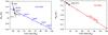 |
Fig. 13 M50 as a function of the core mass for different dust-to-gas ratios and different Ṁmax. The left panel shows the results for a cold start, while the right panel is for a hot start. The black stars correspond to the runs with different Ṁmax, while the diamonds correspond to the runs with different dust-to-gas ratios. |
In the transition region between no deuterium burned at all and complete deuterium
fusion, all objects of one given Ṁmax or dust-to-gas ratio,
but of different total mass, have nearly the same core mass. Thus we are able to plot
M50 against the core mass for the different dust-to-gas
ratios and for the different Ṁmax.
M50 as a function of the core mass for hot and cold start
simulations is shown in Fig. 13. If the varying
amount of burned deuterium in the cold start case for different
Ṁmax was caused by different core masses, then the
Ṁmax simulations should lie on the same line as the
dust-to-gas ratio simulations (the fpg runs). Figure 13 shows that this is not the case, which implies that indeed the accretion at
larger radii is important for objects with larger Ṁmax. For
the hot start objects, in contrast, we find that the dependence of
M50 on Ṁmax can be explained
by different core masses alone, as the Ṁmax runs in
Fig. 13 lie on the same line as the dust-to-gas
ratio runs. It is thus not the case that a different Ṁmax
directly influences the deuterium burning process in the hot start case, but it is a
second order effect that different Ṁmax result in slightly
different core masses. In order to get the deuterium burning mass limit
M50 as a function of the core mass, we fit lines through
the cold start runs with varying dust-to-gas ratio and varying
Ṁmax, as well as through the hot start dust-to-gas ratio
runs. 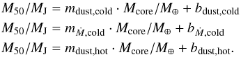 (29)This
yielded the fitting parameters given in Table 5.
(29)This
yielded the fitting parameters given in Table 5.
We find that M50 is approximately equally sensitive to the core masses for both the cold and the hot start scenario: in the core mass range from ~30 M ⊕ to ~100 M ⊕ , M50 decreases by ~0.6 MJ. The y-intercept of the fitted lines furthermore indicates that for objects without a core M50 is 13.58 MJ for a cold start and 13.42 MJ for a hot start in our fiducial model. However, this result should be treated cautiously, as a object formed via the core accretion scenario harbors a solid core at all times during its formation and subsequent evolution in our model (no core erosion) and thus we cannot further test this result. The second reason is that the mass limit M50 for a core mass of 0 M ⊕ is an extrapolation of our data.
6. Distinguishability of cold and hot start objects
As both cold and hot start objects will eventually forget their initial conditions their evolutionary sequences will converge after a certain time, making an observational identification of the accretion mode (i.e. cold or hot start) difficult. The timescale after which the luminosity of a 10 MJ cold start object converges to the luminosity of a 10 MJ hot start object is in the order of 108 to 109 years (Marley et al. 2007). This timescale will increase with mass, which can be understood by looking at the specific entropies of the objects. For hot start objects the specific entropy directly after formation is increasing with mass, whereas the specific entropy of cold start objects is decreasing with mass. As the objects are nearly fully convective the specific entropy can be used as a proxy for the thermodynamic state of the objects. Thus one finds that the difference between the thermodynamic states of cold and hot start objects after formation increases with mass and thus shifts the convergence to later times. In Sect. 5.1.4 we have shown that deuterium burning objects of the same mass would attain the same thermodynamic state if one holds their deuterium abundance artificially constant (the hypothetical “deuterium main sequence”), independent from whether they formed hot or cold. With non-constant deuterium abundance we found that hot and cold start objects will try to attain the “main-sequence”-state, even though they are unable to reach it fully. As both hot and cold start objects tend to attain the same “main-sequence” state it is clear that their thermodynamic properties will start to converge. After having burned up all their deuterium they will then continue the normal evolution, governed by contraction and cooling. This tendency of both hot and cold start objects to attain the same state due to deuterium burning should thus have an influence on the convergence timescale between cold and hot start objects. This is indeed what we find.
First we define the timescale τL as the timescale after which the ratio Lhot/Lcold, where Lhot and Lcold stand for the total luminosity of a hot and cold start object, has reached a value of 1.1 as a function of mass. We considered two cases: for one run deuterium burning was disabled artificially, while for the other run our normal model was used, including deuterium burning. In our fiducial model, we found that for masses between 14 MJ to 21 MJτL increases monotonously as a function of mass for disabled deuterium burning, going from 4 × 10⁸ years to 1.1 × 10⁹ years. For deuterium burning objects it attains a constant value of approximately 2 × 10⁸ years in the same mass range. We thus find that deuterium burning shortens the convergence timescale of massive cold and hot start objects. Nevertheless, one should keep in mind that the exact numerical values of τL depend on the assumptions (e.g. the structure of the accretion shock) and initial conditions used for a model. However, the qualitative behavior should stay the same.
Fitting parameters for M50 as a function of the core mass.
7. Summary
We have studied deuterium burning in objects with masses between 10 to 30 MJ that form via the core accretion mechanism. Such high masses could be reached if gap formation does not act as a limit for gas accretion (Kley & Dirksen 2006), which might be supported by the observational finding that the planetary mass function seems relatively continuous up to a mass of ~25 MJ (Sahlmann et al. 2011). Our simulations self-consistently link the formation and the evolution phase. We have considered two limiting cases for the property of the accretion shock occurring during the gas runaway accretion phase. First, that it is completely radiatively inefficient, so that no liberated gravitational potential energy is radiated away. Instead, high entropy material is incorporated into the object, leading to a so-called hot start. We find that the properties of such objects forming gradually with the core accretion but without radiative losses at the shock are the same as found in the classical hot start simulations where one starts with an already fully formed object with some specified high entropy, usually thought to have formed via direct collapse. This shows that the structure of the shock is as decisive to determine the thermodynamic properties of an object as it’s formation mechanism. Second, we assumed that the shock is fully radiatively efficient so that all potential energy liberated at the shock is radiated away. This leads to low entropy, so-called cold start objects. We have then studied the following topics:
-
Comparison with Burrows et al. (1997)and Spiegel et al. (2011): as seen inSect. 4, we were able to cover the results of Spiegelet al. (2011) for deuterium burning in classicalhot start objects, who started at the final mass at an arbitrary en-tropy without considering the formation. The radii at which theobjects get partially stabilized against contraction as well as thepeak values of LD/Ltot and the temperatures agree very well. The onlydifference is that our objects in the transition zone between nondeuterium burning objects and deuterium burning objects seemto be able to maintain a higher burning rate over a longer periodof time, enabling them to burn more deuterium in total. This isprobably due to different opacities (leading to different coolingtracks) and the high temperature dependence of deuterium burn-ing. Also, looking at the sensitivity of the minimum mass limit ofdeuterium burning in hot start objects, we find approximately thesame slopes for M50 (which is the mass at which 50% of the deuteriumhas been burned) as Spiegel et al. (2011) whenconsidering variations of the helium fraction Y and the deuteriumabundance [D/H] (see Sect. 5.2). In the hot startcase we find a mass limit of M50 = 13.15 MJ for our fiducial model (Y = 0.25, [D/H] = 2 × 10⁻⁵).
-
Behavior of deuterium burning in hot start objects: in addition to the fact that we could reconfirm the results of Spiegel et al. (2011) we were furthermore able to investigate the sensitivity of deuterium burning to quantities linked to the underlying core accretion formation process. We found that deuterium burning in hot start objects is virtually independent of the maximum allowed gas accretion rate Ṁmax and that a higher core mass (determined by the dust-to-gas ratio, i.e. the metallicity of the protoplanetary disk) yields higher central temperatures which will increase the deuterium burning rate. Using our fiducial model, we find that M50 = 13.15MJ for a core mass of 35 M ⊕ and M50 = 12.62MJ for a core mass of 101 M ⊕ . Extrapolation to Mcore = 0 yields M50 = 13.42 MJ.
-
Behavior of deuterium burning in cold start objects: as cold start objects accrete most of their mass at small radii during the runaway phase, they will be below their (hypothetical) deuterium main sequence radius when their central density and temperature become high enough to burn deuterium. The thermostatic nature of deuterium fusion will then cause the objects to expand. Due to the concurrent decrease of deuterium they will not, however, be able to fully reach the hypothetical deuterium main sequence radius. This leads to a re-inflation of the planets to about 1.4 RJ and 2.3 RJ for for a 14 MJ and 23 MJ object, respectively. Objects with masses higher than approximately 23 MJ burn almost all their deuterium during the formation phase (for Ṁmax = 10-2 M ⊕ /yr), as higher masses lead to higher central temperatures and thus higher deuterium burning rates. Objects with masses ≤ 20 MJ burn most of their deuterium after the formation with Ṁmax = 10-2 M ⊕ /yr is complete.
-
Sensitivity of the deuterium burning mass limit: the sensitivity of the minimum mass limit for deuterium burning for cold start objects, M50, is comparable to the hot start objects when considering variations in the helium mass fraction Y, the deuterium abundance [D/H] and the core mass. The dependence is, however, somewhat steeper for cold start objects. For an increase of Y = 0.22 to Y = 0.3, M50 decreases from 13.9 MJ to 12.3 MJ. For an increase of [D/H] from 10-5 to 4 × 10⁻⁵, M50 decreases from 13.6 MJ to 12.9 MJ. When varying the maximum allowed gas accretion rate Ṁmax, the deuterium burning in cold start objects reacts stronger than in the hot start case. The reason for this is that the cold start objects with higher Ṁmax will accrete mass in the runaway phase at larger radii than those with smaller Ṁmax. Accretion onto a larger object means that the accretion shock is weaker, leading to less radiative losses. The object therefore has a higher specific entropy and, quite counterintuitively, burns deuterium more intensively (see Sect. 5.2 and Appendices A and B). Similar as for the hot start, we find (using our fiducial model) that M50 = 13.3MJ for a core mass of 32 M ⊕ and M50 = 12.66 MJ for a core mass of 97 M ⊕ . Extrapolation to Mcore = 0 yields M50 = 13.58 MJ.
-
Evolution of the luminosity: the evolution of the luminosity (as well as the radius and effective temperature) of hot start objects is characterized by a monotonic decrease in time, once the formation process is over. Cold start objects in contrast begin after formation with a luminosity one to two orders of magnitude lower, but then get brighter, due to deuterium burning. The luminosity of hot and cold start objects more massive than ~15 MJ converges after ~200 Myr, due to deuterium burning.
In summary, we find that the transition between deuterium burning and non-deuterium burning objects lies at approximately 13 MJ also for objects forming via the core accretion scenario (see, e.g., Fig. 12), independent of whether they might have formed with a hot or a cold start. The exact behavior of deuterium burning, however, depends on the initial conditions such as the helium mass fraction, the deuterium abundance and the metallicity. Furthermore the exact thermodynamics of the accretion shock (cold start or hot start) and the maximum allowed mass accretion rate during the runaway formation phase play a role. Nevertheless the transition from no deuterium burning at all to complete fusion of all deuterium nuclei always goes from ~10 MJ to ~15 MJ for a realistic range of parameters (see Fig. 10).
8. Conclusion
Deuterium burning so far has been studied in detail only in objects which have not formed via the core accretion scenario (although Baraffe et al. 2008 found that deuterium burning in objects harboring a solid core is possible). It is, however, important to consider deuterium burning as well in objects with a core which have formed via the core accretion scenario, as it cannot be excluded that objects forming in a protoplanetary disk via core accretion can grow beyond the required mass of ~13 MJ (Kley & Dirksen 2006). This scenario is particularly interesting as objects that form via the core accretion scenario in a disk are usually named “planets”. This contradicts the planet definition on deuterium burning alone, leading to an interesting class of deuterium burning planets (Baraffe et al. 2008). Therefore one should consider the possibility of objects with masses in the brown dwarf domain that have a solid core, at least initially, as the exact fate of the core under the extreme conditions in objects as heavy as considered here is uncertain and our results are in the limit that the core is not eroded.
Considering a core accretion formation of the objects in the hot start scenario, we find, when comparing to the results of Spiegel et al. (2011) and Burrows et al. (1997), that such objects with a core burn their deuterium in approximately the same way as the objects without a core. The sensitivity of the burning process to changes in the parameters like Y and [D/H] is approximately also the same (neglecting those parameters which are characteristic to the core accretion scenario).
It is important to note, however, that if an object forms via core accretion and a low initial entropy (cold start) this will considerably alter the way in which the deuterium is burned and how the objects react to it. The biggest difference between the two formation modes is that cold start objects will expand to radii somewhat smaller than the hypothetical deuterium main sequence radius (which would be attained with a constant deuterium abundance). The most massive cold start object considered here (23 MJ) reinflates to a radius larger than 2 RJ, coming from a radius of just over 1 RJ. For hot start objects no reinflation occurs. Future direct imaging observations of young objects, if possible coupled with dynamical mass estimates may allow to observationally test these findings, and to constrain the formation mode of objects at the transition between planets and Brown Dwarfs.
In addition to the results of Spiegel et al. (2011), who found that deuterium burning is depending on the metallicity of the objects via the opacity, it should be kept in mind that the metallicity also determines the core mass (if the local gas surface density in the protoplanetary disk is known). A higher core mass leads to a higher burning rate. Thus this should add up to the opacity related deuterium burning enhancement effect of the metallicity.
Finally we saw that the consideration of a core accretion scenario also yields that the border between deuterium burning and non deuterium burning objects remains at approximately 13 MJ. To model the exact deuterium burning behavior, however, it is important to know certain characteristics of a system, such as the helium abundance, the solid surface density, the deuterium abundance and an upper limit for the gas runaway accretion rate.
Numerical data showing the formation and subsequent evolution of cold and hot start objects in our fiducial model can be found at the CDS and at http://www.mpia.de/homes/mordasini/Site7.html
We start the consideration from the detached phase here as only after the collapse and the subsequent runaway accretion of mass one reaches temperatures and densities high enough to fuse deuterium.
For an ideal gas with an EOS in the form P = (γ − 1)ρu the dependence of ξ on the internal energy content would be expressed as an dependence on γ, the adiabatic index of the gas.
In the terminology used in this paper, by saying “central” we always mean the innermost layer of gas just above the solid core.
Acknowledgments
We thank Hubert Klahr, Yann Alibert and Kai-Martin Dittkrist for helpful discussions. We especially thank David Spiegel and Adam Burrows for dedicated comparison calculations concerning the expansion phase of cold start objects. Finally, we thank our referee Gilles Chabrier for questions which helped us to gain a deeper understanding of the governing physical mechanisms. Christoph Mordasini acknowledges the support as an Alexander von Humboldt fellow.
References
- Alibert, Y., Mordasini, C., & Benz, W. 2004, A&A, 417, L25 [NASA ADS] [CrossRef] [EDP Sciences] [Google Scholar]
- Angulo, C., Arnould, M., Rayet, M., et al. 1999, Nucl. Phys. A, 656, 3 [NASA ADS] [CrossRef] [Google Scholar]
- Baraffe, I., Chabrier, G., & Barman, T. 2008, A&A, 482, 315 [NASA ADS] [CrossRef] [EDP Sciences] [Google Scholar]
- Bodenheimer, P. H., Hubickyj, O., & Lissauer, J. J. 2000, Icarus, 143, 2 [NASA ADS] [CrossRef] [Google Scholar]
- Boss, A. P., Butler, R. P., Hubbard, W. B., et al. 2007, Trans. IAU, Ser. A, 26, 183 [Google Scholar]
- Burrows, A., Marley, M., Hubbard, W. B., et al. 1997, ApJ, 491, 856 [NASA ADS] [CrossRef] [Google Scholar]
- Burrows, A., Hubbard, W. B., Lunine, J. I., & Liebert, J. 2001, Rev. Mod. Phys., 73, 719 [Google Scholar]
- Chabrier, G., & Baraffe, I. 2000, ARA&A, 38, 337 [NASA ADS] [CrossRef] [Google Scholar]
- D’Angelo, G., Durisen, R. H., & Lissauer, J. J. 2010, in Exoplanets, ed. S. Seager (Tucson: Univ. of Arizona Pr.), 319 [Google Scholar]
- Dewitt, H. E., Graboske, H. C., & Cooper, M. S. 1973, ApJ, 181, 439 [NASA ADS] [CrossRef] [Google Scholar]
- Fischer, D. A., & Valenti, J. 2005, ApJ, 622, 1102 [NASA ADS] [CrossRef] [Google Scholar]
- Fowler, W. A., Caughlan, G. R., & Zimmerman, B. A. 1967, ARA&A, 5, 525 [NASA ADS] [CrossRef] [Google Scholar]
- Freedman, R. S., Marley, M. S., & Lodders, K. 2008, ApJS, 174, 504 [NASA ADS] [CrossRef] [Google Scholar]
- Graboske, H. C., Dewitt, H. E., Grossman, A. S., & Cooper, M. S. 1973, ApJ, 181, 457 [NASA ADS] [CrossRef] [Google Scholar]
- Guillot, T., Stevenson, D. J., Hubbard, W. B., & Saumon, D. 2004, in Jupiter, The Planet, Satellites and Magnetosphere, eds. F. Bagenal, T. E. Dowling, & W. B. McKinnon (Cambridge: Cambridge Univ. Press), 35 [Google Scholar]
- Janson, M., Bonavita, M., Klahr, H., et al. 2011, ApJ, 736, 89 [NASA ADS] [CrossRef] [Google Scholar]
- Kippenhahn, R., & Weigert, A. 1990, Stellar Structure and Evolution (Berlin, Heidelberg, New York: Springer Verlag) [Google Scholar]
- Kley, W., & Dirksen, G. 2006, A&A, 447, 369 [NASA ADS] [CrossRef] [EDP Sciences] [Google Scholar]
- Leconte, J., & Chabrier, G. 2012, A&A, 540, A20 [NASA ADS] [CrossRef] [EDP Sciences] [Google Scholar]
- Lodders, K. 2003, ApJ, 591, 1220 [NASA ADS] [CrossRef] [Google Scholar]
- Lubow, S. H., Seibert, M., & Artymowicz, P. 1999, ApJ, 526, 1001 [NASA ADS] [CrossRef] [Google Scholar]
- Marley, M. S., Fortney, J. J., Hubickyj, O., Bodenheimer, P., & Lissauer, J. J. 2007, ApJ, 655, 541 [NASA ADS] [CrossRef] [Google Scholar]
- Mercer-Smith, J. A., Cameron, A. G. W., & Epstein, R. I. 1984, ApJ, 279, 363 [NASA ADS] [CrossRef] [Google Scholar]
- Mordasini, C., Alibert, Y., Klahr, H., & Benz, W. 2011, EPJ Web of Conferences, 11, 4001 [CrossRef] [EDP Sciences] [Google Scholar]
- Mordasini, C., Alibert, Y., Dittkrist, K.-M., et al. 2012, A&A, submitted [Google Scholar]
- Palla, F., Zinnecker, H., Maeder, A., & Meynet, G. 2002, Physics of Star Formation in Galaxies, ed. F. Palla, H. Zinnecker, A. Maeder, & G. Meynet (Berlin, Heidelberg, New York: Springer Verlag) [Google Scholar]
- Pollack, J. B., Hubickyj, O., Bodenheimer, P., et al. 1996, Icarus, 124, 62 [NASA ADS] [CrossRef] [Google Scholar]
- Prodanović, T., Steigman, G., & Fields, B. D. 2010, MNRAS, 406, 1108 [NASA ADS] [Google Scholar]
- Rózyczka, M., Kornet, K., Bodenheimer, P., & Stepinski, T. 2004, Rev. Mex. Astron. Astrof. Conf. Ser., 22, 91 [NASA ADS] [Google Scholar]
- Sahlmann, J., Ségransan, D., Queloz, D., & Udry, S. 2011, IAU Symp. 276, eds. A. Sozzetti, M. G., Lattanzi, & A. P. Boss, 117 [Google Scholar]
- Santos, N. C., Israelian, G., Mayor, M., Rebolo, R., & Udry, S. 2003, A&A, 398, 363 [NASA ADS] [CrossRef] [EDP Sciences] [Google Scholar]
- Saumon, D., Chabrier, G., & van Horn, H. M. 1995, ApJS, 99, 713 [NASA ADS] [CrossRef] [Google Scholar]
- Saumon, D., Hubbard, W. B., Burrows, A., et al. 1996, ApJ, 460, 993 [NASA ADS] [CrossRef] [Google Scholar]
- Ségransan, D., Udry, S., Mayor, M., et al. 2010, A&A, 511, A45 [NASA ADS] [CrossRef] [EDP Sciences] [Google Scholar]
- Spergel, D. N., Bean, R., Doré, O., et al. 2007, ApJS, 170, 377 [NASA ADS] [CrossRef] [Google Scholar]
- Spiegel, D. S., & Burrows, A. 2012, ApJ, 745, 174 [NASA ADS] [CrossRef] [Google Scholar]
- Spiegel, D. S., Burrows, A., & Milsom, J. A. 2011, ApJ, 727, 57 [NASA ADS] [CrossRef] [Google Scholar]
- Stahler, S. W. 1988, ApJ, 332, 804 [NASA ADS] [CrossRef] [Google Scholar]
- Stahler, S. W., Shu, F. H., & Taam, R. E. 1980, ApJ, 241, 637 [NASA ADS] [CrossRef] [Google Scholar]
- Wilson, H. F., & Militzer, B. 2012, ApJ, 745, 54 [NASA ADS] [CrossRef] [Google Scholar]
Appendix A: Envelope cooling due to the core
The goal of this approximation is to show that even an ideal gas in the envelope will
eventually cool in the presence of a solid core. From the usual analysis without a core
one obtains that
Tcent ∝ 1/R (see
Eq. (23)). In order to show this we make
a virial analysis. Assuming virial equilibrium of the envelope we can start with the
equation of hydrostatic equilibrium
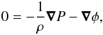 (A.1)where
P is the pressure, ρ the density and
φ the gravitational potential. We assume the gas in the envelope to be
ideal. Furthermore we assume that the core density is constant. In this idealized
analysis, one writes
(A.1)where
P is the pressure, ρ the density and
φ the gravitational potential. We assume the gas in the envelope to be
ideal. Furthermore we assume that the core density is constant. In this idealized
analysis, one writes 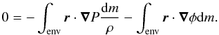 (A.2)We integrate over the
envelope only as we are interested in the envelope only. The core is merely treated as an
external factor; this also means that the second integral on the RHS of the above equation
contains the potential energy of the envelope in the gravitational field of the core, but
not the potential energy of the core itself. Using
dm/ρ = dV the
first integral on the RHS of Eq. (A.2)
transforms to
(A.2)We integrate over the
envelope only as we are interested in the envelope only. The core is merely treated as an
external factor; this also means that the second integral on the RHS of the above equation
contains the potential energy of the envelope in the gravitational field of the core, but
not the potential energy of the core itself. Using
dm/ρ = dV the
first integral on the RHS of Eq. (A.2)
transforms to 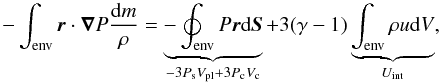 (A.3)where
dS is an infinitesimal vectorial surface element of the
envelope, γ is the adiabatic index and u is the specific
energy density of the gas. Ps is the surface pressure which is
negligible in our problem, Vpl is the object’s volume,
Pc is the gas pressure on top of the core,
Vc is the core volume and Uint
denotes the internal energy of the envelope. Furthermore one can show that the second term
on the RHS of Eq. (A.2) is equal to the
gravitational potential energy W of the envelope with
(A.3)where
dS is an infinitesimal vectorial surface element of the
envelope, γ is the adiabatic index and u is the specific
energy density of the gas. Ps is the surface pressure which is
negligible in our problem, Vpl is the object’s volume,
Pc is the gas pressure on top of the core,
Vc is the core volume and Uint
denotes the internal energy of the envelope. Furthermore one can show that the second term
on the RHS of Eq. (A.2) is equal to the
gravitational potential energy W of the envelope with
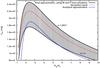 |
Fig. A.1 Internal energy of the envelope obtained from the simulation (red dotted line), the internal energy obtained by using the potential energy and the pressure from the simulation in Eq. (A.5) for the two limiting γ (black solid line) and the internal energy obtained by using the fully analytical approximation from Eq. (A.9) and γ = 1.2857 (blue dot-dashed line). The gray area shows where one would expect the internal energy (red dotted line) to be. |
 (A.4)where
Wenv−core is the potential energy of the envelope in the
gravitational field of the core and Wenv−env is the
potential energy of the envelope due to its own gravitational field. Thus we finally have
(A.4)where
Wenv−core is the potential energy of the envelope in the
gravitational field of the core and Wenv−env is the
potential energy of the envelope due to its own gravitational field. Thus we finally have
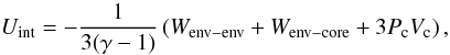 (A.5)We furthermore found
that Wenv−env is reasonably well described by
(A.5)We furthermore found
that Wenv−env is reasonably well described by 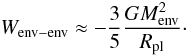 (A.6)Wenv−corecan
be estimated by
(A.6)Wenv−corecan
be estimated by 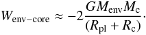 (A.7)To approximate
the core pressure we use the equation of hydrostatic equilibrium again and neglect all
terms linear in the core mass. One then finds
(A.7)To approximate
the core pressure we use the equation of hydrostatic equilibrium again and neglect all
terms linear in the core mass. One then finds  (A.8)Again using that
Ps is negligible one finally gets by using Eq. (A.5), (A.6) and (A.8):
(A.8)Again using that
Ps is negligible one finally gets by using Eq. (A.5), (A.6) and (A.8):
 (A.9)With
this approach one finds that the envelope starts to cool if the
Rpl becomes smaller than
2.83 Rc if Mc → 0 and somewhat
later for non negligible core masses. The physical reason for this cooling process is that
the excess energy is transferred to the core which has to withstand an evergrowing
external pressure. In order to test this approximation we carried out a simulation forming
a 1 MJ planet, using a constant core density as well as an
ideal H2 EOS for the envelope. γ then varies between 1.4 near
the surface and 1.2857 at the center. The core mass was
35 M ⊕ . In Fig. A.1
one can see the internal energy of the envelope obtained from the simulation, the internal
energy obtained by using the potential energy and the pressure from the simulation in
Eq. (A.5) and the internal energy
obtained by using the fully analytical approximation from Eq. (A.9) and γ = 1.2857. One sees
that the analytical approximations recover the shape of the internal energy curve obtained
from the simulation quite well. Furthermore the simulation result is bracketed by the two
results obtained from Eq. (A.5) using
γ = 1.4 and γ = 1.2857.
(A.9)With
this approach one finds that the envelope starts to cool if the
Rpl becomes smaller than
2.83 Rc if Mc → 0 and somewhat
later for non negligible core masses. The physical reason for this cooling process is that
the excess energy is transferred to the core which has to withstand an evergrowing
external pressure. In order to test this approximation we carried out a simulation forming
a 1 MJ planet, using a constant core density as well as an
ideal H2 EOS for the envelope. γ then varies between 1.4 near
the surface and 1.2857 at the center. The core mass was
35 M ⊕ . In Fig. A.1
one can see the internal energy of the envelope obtained from the simulation, the internal
energy obtained by using the potential energy and the pressure from the simulation in
Eq. (A.5) and the internal energy
obtained by using the fully analytical approximation from Eq. (A.9) and γ = 1.2857. One sees
that the analytical approximations recover the shape of the internal energy curve obtained
from the simulation quite well. Furthermore the simulation result is bracketed by the two
results obtained from Eq. (A.5) using
γ = 1.4 and γ = 1.2857.
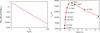 |
Fig. A.2 Left panel: analytical approximation of the derivative of the internal energy of the ions with respect to the object’s radius plotted against Rpl/Rc. Right panel: central temperature (i.e. the temperature in the envelope above the core) of a 10 MJ hot start planet as a function of Rpl. t0 denotes the time where the formation of the object is finished. |
Appendix B: Envelope cooling due to the core and the electron degeneracy
It is well known that the ions in fully degenerate objects, such as White Dwarfs, will
cool as they contract. The excess energy is put into the degenerate electrons. In the
objects considered in this paper we have partially degenerate envelopes. However, in order
to make an analytical analysis simpler, we will consider a fully degenerate envelope. In
combination with the effect that the presence of the core can already cool an ideal gas
envelope we expect a cooling behaviour for the degenerate envelope as well. We use the
simplification that the internal energy of the electrons is approximately
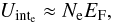 (B.1)where
EF is the Fermi energy and Ne
the number of electrons. Next we use that
(B.1)where
EF is the Fermi energy and Ne
the number of electrons. Next we use that  and
and
 ,
where pF is the Fermi momentum and
ne the electron number density. As
,
where pF is the Fermi momentum and
ne the electron number density. As
 one finally obtains that
 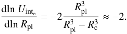 (B.2)Here we made the
approximation that
(B.2)Here we made the
approximation that  , which is
justified in the case considered here as degenerate envelopes do not contract as much as
the ideal ones do. Furthermore it holds for the potential energy of the envelope
, which is
justified in the case considered here as degenerate envelopes do not contract as much as
the ideal ones do. Furthermore it holds for the potential energy of the envelope
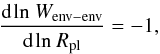 (B.3)which yields,
together with Eq. (B.2):
(B.3)which yields,
together with Eq. (B.2): 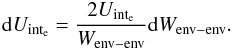 (B.4)We use that the
ions can be considered as an ideal gas. Then it holds for both the ions and the degenerate
electrons that P = 2/3ρu. One finds
again from a virial analysis that one can write then
(B.4)We use that the
ions can be considered as an ideal gas. Then it holds for both the ions and the degenerate
electrons that P = 2/3ρu. One finds
again from a virial analysis that one can write then 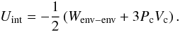 (B.5)Here we neglected
Wenv−core this time since for the objects we are
ultimately interested in, it holds that
Menv ≫ Mc. As we consider a
fully degenerate envelope the internal energy of the electrons should be much larger than
the internal energy of the ions:
(B.5)Here we neglected
Wenv−core this time since for the objects we are
ultimately interested in, it holds that
Menv ≫ Mc. As we consider a
fully degenerate envelope the internal energy of the electrons should be much larger than
the internal energy of the ions:  (B.6)Thus one finds from
Eq. (B.5):
(B.6)Thus one finds from
Eq. (B.5):
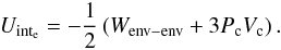 (B.7)From Eqs. (A.6) and (A.8) we know that
  (B.8)with
 (B.9)For the change of the
internal energy
dUint = dUinte + dUintI
we now find
(B.9)For the change of the
internal energy
dUint = dUinte + dUintI
we now find  (B.10)Using Eqs. (B.4) and (B.8) then yields
 (B.11)As the only free
parameter for a given object is Rpl (i.e.
Menv and Rc are fixed) one finds
the above equation to be equal to
(B.11)As the only free
parameter for a given object is Rpl (i.e.
Menv and Rc are fixed) one finds
the above equation to be equal to
![Mathematical equation: \appendix \setcounter{section}{2} \begin{equation} {\rm d}U_{\rm int_I}=\left[\left(\frac{1}{2}-K_R\right) \frac{{\rm d} W_{\rm env-env}}{{\rm d} R_{\rm pl}}+\frac{1}{2}\frac{{\rm d} (W_{\rm env-env}K_R)}{{\rm d} R_{\rm pl}}\right]{\rm d} R_{\rm pl} . \end{equation}](/articles/aa/full_html/2012/11/aa19844-12/aa19844-12-eq276.png) (B.12)For the cooling of the
ions one must have
(B.12)For the cooling of the
ions one must have  (B.13)and therefore
 (B.14)which means that the
internal energy of the ions decreases as the objects shrink. In the left panel of
Fig. A.2 one can see that this is indeed the case,
i.e. we expect the degenerate envelope around the solid core to cool. For a partly
degenerate envelope however, if the objects radius is much larger than the cooling radius
derived for ideal gas (2.83 Rc), the object should heat up
during contraction. The reason for this is that the degeneracy in the envelope is not yet
strong enough to result in ion cooling. In the right panel of Fig. A.2 one sees the central temperature (i.e. the temperature in the
envelope above the core) of a 10 MJ hot start planet as a
function of the radius for the whole post-formation phase (starting at time
t0). The envelope EOS is the EOS of Saumon et al. (1995), and the core density was not kept constant
artificially. One can see that the envelope heats up until it has reached a radius of
approximately 1.7 RJ and then cools down. Non
deuterium burning cold start objects will always cool in the post formation phase as they
are already strongly degenerate.
(B.14)which means that the
internal energy of the ions decreases as the objects shrink. In the left panel of
Fig. A.2 one can see that this is indeed the case,
i.e. we expect the degenerate envelope around the solid core to cool. For a partly
degenerate envelope however, if the objects radius is much larger than the cooling radius
derived for ideal gas (2.83 Rc), the object should heat up
during contraction. The reason for this is that the degeneracy in the envelope is not yet
strong enough to result in ion cooling. In the right panel of Fig. A.2 one sees the central temperature (i.e. the temperature in the
envelope above the core) of a 10 MJ hot start planet as a
function of the radius for the whole post-formation phase (starting at time
t0). The envelope EOS is the EOS of Saumon et al. (1995), and the core density was not kept constant
artificially. One can see that the envelope heats up until it has reached a radius of
approximately 1.7 RJ and then cools down. Non
deuterium burning cold start objects will always cool in the post formation phase as they
are already strongly degenerate.
All Tables
All Figures
|
Fig. 1 Temporal evolution of the luminosity (upper left), the radius (upper right), the entropy above the core (lower left) and the mass averaged Θe-factor in the envelope (lower right) for hot start objects with masses varying from 10 MJ to 30 MJ using our fiducial model as defined in Table 1. The black dashed line in all plots corresponds to the 13 MJ object. The masses corresponding to the individual lines are indicated in the plot. The horizontal green line in the plot of the radius indicates the position of 1 RJ. |
| In the text | |
|
Fig. 2 Radial evolution of deuterium burning objects (hot start accretion). The solid red lines show our own results, whereas the dashed green lines show the results of Burrows et al. (1997). As the t = 0 definition is not the same, the Burrows et al. (1997) results where shifted in time in order to make the phases of deuterium burning coincide. The mass of the objects is indicated in the plots. |
| In the text | |
|
Fig. 3 Left column: the ratio LD/Ltot. Right column: the depletion of deuterium. The first row shows our results for different helium abundances, the second row shows the influence of different deuterium abundances and the last row shows different dust-to-gas ratios (as defined in Table 2). The mass of all objects is 13 MJ (hot start). The run names corresponding to the individual lines are indicated in the plot. |
| In the text | |
|
Fig. 4 Left panel: the ratio LD/Ltot as a function of time. Right panel: the depletion of deuterium for the runs with different maximum allowed mass accretion rates (as defined in Table 2). The mass of the objects is 13 MJ (hot start). The run names corresponding to the individual lines are indicated in the plot. |
| In the text | |
|
Fig. 5 Central temperature for the different dust-to-gas ratio runs (left plot) and for the different maximum allowed gas accretion runs (right plot) (hot start). |
| In the text | |
|
Fig. 6 Formation and subsequent evolution of a 16 MJ object forming via core accretion with a radiatively efficient shock (cold start). The four panels show the temporal evolution of the total luminosity (internal + shock) (upper left), the radius (upper right), the central temperature (lower left) and the surface temperature (lower right). The dotted blue line shows the results obtained for the fiducial model as specified in Table 1. For the solid red line, the deuterium abundance was kept constant, while for the dashed green line, deuterium burning was disabled. |
| In the text | |
|
Fig. 7 Radius as a function of time for objects forming via the hot start ansatz (solid line) or the cold start ansatz (dashed line). The mass of the objects is indicated in each panel. In the upper right panel (16 MJ) the gray lines show the results obtained for a constant deuterium abundance. |
| In the text | |
|
Fig. 8 Temporal evolution (for cold start objects) of the luminosity as seen by an observer, i.e. including the accretion luminosity (first row, left), the surface temperature (first row, right), the radius (second row, left), the gravitational acceleration at the surface (second row, right), the specific entropy above the core (third row, left) and the degeneracy related factor Θe (third row, right) for objects with masses varying from 10 MJ to 23 MJ using our fiducial model as defined in Table 1. The black dashed line in all plots corresponds to the 13 MJ object. The horizontal green line in the plot of the radius indicates the position of 1 RJ. The masses corresponding to the lines are indicated in the plot. |
| In the text | |
|
Fig. 9 Evolution of the luminosities of cold start objects with masses as indicated in the plot. The blue solid lines show the total luminosities of the objects (i.e. the luminosity an observer would see), whereas the dashed red lines denote the luminosity due to deuterium burning only. The luminosities for the different masses have been separated in the y-axis by an arbitrary offset for better visibility. Up to approximately 1.3 × 10⁶ years, where the gas runaway accretion ends for the 13 MJ object, all objects have the same luminosity. |
| In the text | |
|
Fig. 10 Fraction of the initial deuterium burned as a function of mass until the end of the simulation (1010 years) for cold start objects. Top left: results for different helium fractions. Top right: results with different dust-to-gas ratios (or metallicities). Bottom left: results for different maximum gas accretion rates. Bottom right: results for different deuterium abundances. The uppermost run names in the plots correspond to the leftmost curves, the next lower run names correspond to the second leftmost curves etc. For the Y30 run in the upper left panel the positions of the individual mass runs are indicated with filled brown circles. For the sake of clarity we omitted plotting the individual mass run positions for all other runs. Instead a spline function was plotted through the individual mass run positions. |
| In the text | |
|
Fig. 11 Central temperature of a 7 MJ planet as a function of it’s specific entropy showing the complete post-formation evolutionary phase. |
| In the text | |
|
Fig. 12 Masses at which 50% of the deuterium has been burned by 1010 years. Upper row, left: varied helium fraction. Right: varied metallicities. Lower row, left: varied maximum gas accretion rates. Right: varied deuterium abundances. The red dashed line shows the fitted functions for the hot start objects (lower line in all plots), while the fits for the cold start objects are plotted in a blue solid line (upper line in all plots). The blue diamonds show the positions of M50 in the cold start runs, while the red semi-filled circles show the positions of M50 for the hot start runs. |
| In the text | |
|
Fig. 13 M50 as a function of the core mass for different dust-to-gas ratios and different Ṁmax. The left panel shows the results for a cold start, while the right panel is for a hot start. The black stars correspond to the runs with different Ṁmax, while the diamonds correspond to the runs with different dust-to-gas ratios. |
| In the text | |
|
Fig. A.1 Internal energy of the envelope obtained from the simulation (red dotted line), the internal energy obtained by using the potential energy and the pressure from the simulation in Eq. (A.5) for the two limiting γ (black solid line) and the internal energy obtained by using the fully analytical approximation from Eq. (A.9) and γ = 1.2857 (blue dot-dashed line). The gray area shows where one would expect the internal energy (red dotted line) to be. |
| In the text | |
|
Fig. A.2 Left panel: analytical approximation of the derivative of the internal energy of the ions with respect to the object’s radius plotted against Rpl/Rc. Right panel: central temperature (i.e. the temperature in the envelope above the core) of a 10 MJ hot start planet as a function of Rpl. t0 denotes the time where the formation of the object is finished. |
| In the text | |
Current usage metrics show cumulative count of Article Views (full-text article views including HTML views, PDF and ePub downloads, according to the available data) and Abstracts Views on Vision4Press platform.
Data correspond to usage on the plateform after 2015. The current usage metrics is available 48-96 hours after online publication and is updated daily on week days.
Initial download of the metrics may take a while.