| Issue |
A&A
Volume 547, November 2012
|
|
|---|---|---|
| Article Number | A112 | |
| Number of page(s) | 36 | |
| Section | Planets and planetary systems | |
| DOI | https://doi.org/10.1051/0004-6361/201118464 | |
| Published online | 08 November 2012 | |
Characterization of exoplanets from their formation
II. The planetary mass-radius relationship⋆
1
Max-Planck-Institut für Astronomie,
Königstuhl 17,
69117
Heidelberg,
Germany
e-mail: This email address is being protected from spambots. You need JavaScript enabled to view it.
2
Center for space and habitability, Physikalisches Institut,
University of Bern, Sidlerstrasse
5, 3012
Bern,
Switzerland
3
Centre de Recherche Astrophysique de Lyon (CRAL), Ecole Nationale
Supérieure, 46 Allée d’Italie, 69364
Lyon Cedex 07,
France
Received:
15
November
2011
Accepted:
26
August
2012
Abstract
Context. The research of extrasolar planets has entered an era in which we characterize extrasolar planets. This has become possible with measurements of the radii of transiting planets and of the luminosity of planets observed by direct imaging. Meanwhile, the precision of radial velocity surveys makes it possible to discover not only giant planets but also very low-mass ones.
Aims. Uniting all these different observational constraints into one coherent picture to better understand planet formation is an important and simultaneously difficult undertaking. One approach is to develop a theoretical model that can make testable predictions for all these observational techniques. Our goal is to have such a model and use it in population synthesis calculations.
Methods. In a companion paper, we described how we have extended our formation model into a self-consistently coupled formation and evolution model. In this second paper, we first continue with the model description. We describe how we calculate the internal structure of the solid core of the planet and include radiogenic heating. We also introduce an upgrade of the protoplanetary disk model. Finally, we use the upgraded model in population synthesis calculations.
Results. We present how the planetary mass-radius relationship of planets with primordial H2/He envelopes forms and evolves in time. The basic shape of the mass-radius relationship can be understood from the core accretion model. Low-mass planets cannot bind massive envelopes, while super-critical cores necessarily trigger runway gas accretion, leading to “forbidden” zones in the M − R plane. For a given mass, there is a considerable diversity of radii, mainly due to different bulk compositions, reflecting different formation histories. We compare the synthetic M − R plane with the observed one, finding good agreement for a > 0.1 AU. The synthetic planetary radius distribution is characterized by a strong increase towards small R and a second, lower local maximum at about 1 RX. The increase towards small radii comes from the increase of the mass function towards low M. The second local maximum is due to the fact that radii are nearly independent of mass for giant planets. A comparison of the synthetic radius distribution with Kepler data shows good agreement for R ≳ 2 R⊕, but divergence for smaller radii. This indicates that for R ≳ 2 R⊕ the radius distribution can be described with planets with primordial H2/He atmospheres, while at smaller radii, planets of a different nature dominate. We predict that in the next few years, Kepler will find the second local maximum at about 1 RX.
Conclusions. With the updated model, we can compute the most important quantities, like mass, semimajor axis, radius, and luminosity, which characterize an extrasolar planet self-consistently from its formation. The comparison of the radii of the synthetic planets with observations makes it possible to better constrain this formation process and to distinguish between fundamental types of planets.
Key words: planetary systems / planet-disk interactions / planets and satellites: formation / planets and satellites: interiors / planets and satellites: individual: Jupiter / methods: numerical
Appendices A and B are available in electronic form at http://www.aanda.org
© ESO, 2012
1. Introduction
In the first part of this paper, we continue to present the improvement of our formation model in order to extend it into a combined planet formation and evolution model. With these extensions and those introduced in the companion paper (Mordasini et al. 2012b, hereafter Paper I), we are able to synthesize planetary populations for which we can calculate in a self-consistent way not only the mass and semimajor axis as in previous works (e.g., Mordasini et al. 2009a; Alibert et al. 2011) but also the radius and luminosity. This is possible during the entire formation and evolution, starting at a tiny sub-Earth mass seed embryo and ending at a gigayear-old planet. In the second part of the paper, we use population synthesis calculations to study different aspects of the planetary mass-radius (M − R) relationship and the distribution of the radii of the planets.
This work was motivated by the rapidly increasing number of known transiting extrasolar planets in the past few years. Recently, the space missions Convection Rotation and planetary Transits (CoRoT) and Kepler yielded very precise measurements of the radius of a very large number of planet candidates (Léger et al. 2009; Borucki et al. 2011; Batalha et al. 2012). The data from the Kepler satellite has stimulated a multitude of studies such as Howard et al. (2012); Traub (2011); Demory & Seager (2011); Youdin (2011); Wolfgang & Laughlin (2012), and Gaidos et al. (2012), to name just a few. The results of these studies will be used in this work to compare the radii of the actual and the synthetic population.
For a number of transiting planets, masses were measured using the radial velocity (RV) method (e.g., Bouchy et al. 2011) or transit timing variations (e.g., Cochran et al. 2011). The combination of the mass and the radius of the planet yields the planetary M − R diagram, which is an observational result of importance similar to the planetary semimajor axis-mass diagram. The reason for this is that one can derive the mean density of the planet, which constrains, at least to some extent, the internal structure that is crucial to understand the nature (e.g., Chabrier et al. 2011) and, as we shall see in this work, the formation of a planet. We thus make an important step toward a physical characterization of planets based on their formation history.
The radius adds a whole new class of observational constraints, which the output of the theoretical model in a population synthesis can be compared to. Important examples are radius distribution, M − R relationship, and the impact of semimajor axis, metallicity, and stellar mass on the radii. Due to the complexity of planet formation and evolution with a multitude of interacting effects (often only understood in a rudimentary way), it is of highest importance to have as many observational constraints that can concurrently and self-consistently be used for comparison with the theoretical results. This is the central motivation for the present work and the companion paper. The combination of results of different observational techniques makes it possible to obtain insights that could not be obtained from the data of one technique alone (e.g., Wolfgang & Laughlin 2012; Gaidos et al. 2012).
The reason to improve the model of the protoplanetary disk is, on the one hand, the observational progress that has been made in the last few years in this field (e.g., Andrews et al. 2009, 2010; Fedele et al. 2010) as well as also the theoretical result that the disk structure is very important for the final properties of a synthetic planetary population (Mordasini et al. 2012a).
Planetary population synthesis has become possible thanks to the large number of extrasolar planets that have been detected in the last decade. Apart from our series of works, several other studies have been presented (e.g., Ida & Lin 2004, 2010; Thommes et al. 2008; Miguel et al. 2011; Hellary & Nelson 2012). These studies can roughly be divided into two classes, one emphasizing the coupling of several processes (solid and gas accretion, migration, disk evolution), the other treating in detail the N-body interaction. Here, we add long-term evolution in order to allow physical characterization as an additional aspect. In future a natural extension of this approach will be a better description of the atmospheric structure and the chemical composition of the planets, as well as the inclusion of atmospheric evaporation and the formation of secondary atmospheres for low-mass planets. This will finally lead to the study of planetary habitability.
It is the goal of population synthesis to eventually calculate from first physical principles a synthetic population that is able to reproduce in a statistically significant way the observed properties of the actual population in terms of its major characteristics, such as mass, semimajor axis, eccentricity, composition, radius, and luminosity. The formation model used here for the syntheses combines several simple standard descriptions for important physical mechanisms acting during planet formation (α-disk model, core accretion mechanism, tidal migration, 1D planetary structure equations). It is important to understand to what extent this much simplified approach is sufficient to reach the goal. Comparisons with as many observational results as possible should make it possible to identify which aspects of current planet formation and evolution theory need most improvement. We also want to understand if physical mechanisms, which are currently not at all included in the model, are necessary in order to explain the observed properties. Just one example among many is the interaction of planetary systems with third external bodies which causes Kozai migration (Fabrycky & Tremaine 2007) or dynamical instabilities (Malmberg et al. 2011).
In related papers, we present how we have concurrently improved other aspects of our original formation model (Alibert et al. 2004, 2005). We worked on the inclusion of stellar irradiation for the temperature structure of the protoplanetary disk (Fouchet et al. 2012), the description of disk migration taking into account non-isothermal type I migration (Dittkrist et al., in prep.), the concurrent formation of many planets in one disk (Alibert et al., in prep.), and a more realistic planetesimal disk and solid accretion rate (Fortier et al. 2012).
1.1. Structure of the papers
In Paper I, we presented improvements and extensions regarding the calculation of the gaseous envelope of a planet. We introduced a new, simple, and stable method to calculate planetary cooling tracks. We also described the boundary conditions that are used to solve the structure equations.
In Paper I, we used the upgraded model to study the in situ formation and evolution of Jupiter, the radius of giant planets as function of their mass and age, the influence of the core mass on the radius of giant planets, and the planetary luminosity both in the “hot start” and the “cold start” scenario. We put special emphasis on the comparison of our results with those of other models of planet formation and evolution like Burrows et al. (1997), Baraffe et al. (2003), Fortney et al. (2007), and Lissauer et al. (2009). We found that our results agree very well with those of the more complex models, despite the number of simplifications that we made.
In this second paper, we introduce further improvements. In Sect. 2, we describe two upgrades of the computational module which describe the planetary interior structure. First, we solve the internal structure equations of the solid core1, which yields a variable, realistic core density as a function of core mass, core composition, and external pressure by the surrounding envelope (Sect. 2.1). We assume that the planet is differentiated, consisting of iron, silicates, and, if it accreted outside the ice line, ices. The ice line corresponds to the orbital distance in the protoplanetary disk where the temperature drops below the level necessary for ices to condense, see, e.g., Hayashi (1981). Second, we include radiogenic heating due to the decay of long-lived radionuclides in the mantle of the planet (Sect. 2.3). These extensions should make it possible to also calculate the evolution of planets of a relatively low mass, provided that they have a primordial H2/He atmosphere. In Sect. 3, we show how we have improved the disk model by using more realistic initial and boundary conditions as well as a detailed model for the photoevaporation of the disk.
In the following sections, we present our results. We first use the upgrades to study the effect of variable core density on the in situ formation and evolution of Jupiter (Sect. 5). Then we simulate the formation and evolution of a close-in super-Earth2 planet under the influence of radiogenic heating (Sect. 6). As in Paper I, we want to validate the model by comparison with previous studies. Our goal is also to understand how these mechanisms potentially influence population synthesis calculations. The degree of uncertainty that affects our radius calculation is estimated in Sect. 2.2. The most important result, which is the application of the updated model in population synthesis calculations to obtain the planetary M − R relationship, is shown in Sect. 7. We study how the planetary M − R relationship forms and evolves (Sect. 7.2). We show the predicted planetary radius distribution and compare it with the results of the Kepler satellite (Sect. 7.5). We study the impact of the semimajor axis on the radius distribution and give, for comparison with observations, an analytical expression for the mean planetary radius as function of mass (Sect. 7.8). We quantify the spread in radii for a given mass interval in Sect. 7.7 and compare core and total radii in Sect. 7.10. In Sect. 8 we summarize our results, and in Sect. 9, we present the conclusions.
In the Appendix, we show our results concerning the disk module, which are mainly comparisons with previous works. The stability of α disks with the new initial profile against self-gravity is discussed in Appendix A, while the evolution of the disks with the new photoevaporation model is shown in Appendix B.
2. Planet model
2.1. Variable core density
In previous versions of the formation model, we assumed as other formation models a constant core density of 3.2 g/cm3, independent of the size and composition of the core. In order to obtain realistic radii for the core, we have replaced this assumption with an internal structure model. Our model is simpler than the one presented, e.g., by Valencia et al. (2006), and includes, for example, no internal temperature profile. However, as noted by Seager et al. (2007), it nevertheless yields reasonably accurate results for the radius (see Sect. 2.2 for a discussion of the uncertainties).
For low-mass, core-dominated planets (or planets without a significant atmosphere), this means that we have realistic total radii, which is important for comparison with, e.g., Kepler results (Sect. 7.6).
The model calculating the core radii was originally developed for the study of GJ 436b in Figueira et al. (2009), where the methods are described. Our approach is very similar to the one described in Fortney et al. (2007) for solid planets. We assume that the core is differentiated and consists of layers of iron/nickel, silicates, and, if the embryo accreted planetesimals beyond the iceline, (water) ice. The silicate-iron/nickel ratio is fixed to 2:1 in mass as found for the Earth (we shall call such a ratio “rocky”), and the ice fraction is given by the formation model according to whether the planet accretes in- or outside the iceline.
Ordinary chondrites have typical total iron weight fractions of roughly 20 to 30% (Kallemeyn et al. 1989), and carbonaceous chondrites have Fe/Ni weight fractions around 25% (Mason 1963). Therefore, assuming 33% as a typical (not strongly altered by giant impacts, cf. Marcus et al. 2009) iron fraction for rocky planets is probably not far from what is expected for the typical solar abundance mix, although at the upper end (cf. also Weidenschilling 1977).
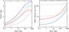 |
Fig. 1 Total planetary or core radii and mean densities as a function of mass for different compositions. The red solid curve corresponds to a rocky planet with a 2:1 silicate-to-iron ratio, similar to Earth. The green dotted curve is for planets consisting of 50% ice, 33% silicates and 17% iron. The blue dashed line shows radii for planets consisting entirely of ice. These three models are calculated without an external pressure on the surface and, therefore, apply to low-mass planets without significant envelopes. The thin red and blue dotted lines show the result from Seager et al. (2007) for comparison. The thin black lines correspond to cores of giant planets. The short-dashed-dotted line is for a 75% ice, 25% rocky core inside an old, Jovian mass planet (Pext = 4 × 10¹³ dyn/cm2). The long-dashed-dotted line is for a core of the same composition inside an old, 10 MX super-Jupiter planet (Pext = 6 × 10¹⁵ dyn/cm2). |
An important effect for the size of cores of giant planets is the external pressure exerted by the envelope. This leads to significant compression of the core for massive planets (Baraffe et al. 2008), where the core is buried below hundreds, or even thousands of Earth masses of gas, and subject to huge pressures of thousands of GPa. This effect is included in our calculations.
While we used in Figueira et al. (2009) the
equation of state (EOS) for solid materials from Fortney et al. (2007), which are more accurate but applicable in a limited pressure
domain only, we now use the slightly less accurate, but more widely applicable (also at
very high pressures) modified polytropic EOS from Seager et al. (2007), which has a form (ρ is the density,
P the pressure)  (1)where the parameters
ρ0, c, and n are given in
Seager et al. (2007). For silicates, we use the
parameters appropriate for MgSiO3 (perovskite). At high pressures, such an EOS
becomes equivalent to a completely degenerate, non-relativistic electron gas (Zapolsky
& Salpeter 1969), which can be used to
solve the Lane-Emden equation with an external pressure (Milne 1936). Regarding the cores of giant planets, we assume for simplicity
that they do not dissolve in the envelope even during the long-term evolution, though this
seems possible (Guillot et al. 2004; Wilson
& Militzer 2012).
(1)where the parameters
ρ0, c, and n are given in
Seager et al. (2007). For silicates, we use the
parameters appropriate for MgSiO3 (perovskite). At high pressures, such an EOS
becomes equivalent to a completely degenerate, non-relativistic electron gas (Zapolsky
& Salpeter 1969), which can be used to
solve the Lane-Emden equation with an external pressure (Milne 1936). Regarding the cores of giant planets, we assume for simplicity
that they do not dissolve in the envelope even during the long-term evolution, though this
seems possible (Guillot et al. 2004; Wilson
& Militzer 2012).
2.1.1. Core radius as a function of core mass
In the left-hand panel of Fig. 1 we show the classical plot of (core) radius versus mass for various compositions (e.g., Zapolsky & Salpeter 1969; Stevenson 1982; Seager et al. 2007; Fortney et al. 2007). It shows first the increase of the radius with mass until a maximum is reached and then a decrease as the electrons become increasingly degenerated and the material more compressible. The right-hand panel shows the corresponding mean densities.
The red solid curve applies to planets with a purely rocky composition (2:1 silicate-to-iron ratio), close to the terrestrial composition. For M = 1 M⊕, the model yields a radius of 0.96 R⊕. The green dotted curve is for 50% ice and 50% rocky, while the dashed blue line is for a planet made purely of water ice, which is a composition that is, however, not expected to exist in nature. All three cases were calculated without applying an external pressure Pext and thus correspond to terrestrial (or ice) planets without significant envelopes. In the left-hand panel, we also show the result of Seager et al. (2007) for planets with a rocky and pure water composition calculated with a more accurate EOS. One sees that for masses less than ~200 M⊕ and ~60 M⊕ for rocky and pure ice planets, respectively, we find very similar radii and recover their results to typically within 1% to 2%. For a pure ice planet, at a mass of 100 M⊕, we find a radius that is 3% smaller than obtained by Seager et al. (2007). At such a high mass, it is, however, expected that a non-negligible amount of gas is accreted during the presence of the protoplanetary disk, which has a much stronger effect on the (total) radius. In the population synthesis at a core mass of 100 M⊕, even planets that accreted the lowest amount of gas have a total radius that is 65% larger than the core radius (cf. Fig. 16).
The two black lines correspond to cores of giant planets. Both lines show the radius for objects consisting of 75% ice and 25% rocky material, as expected for the composition of solids in the solar system beyond the iceline (we shall call such a composition “icy”). This 3:1 ice-to-rock ratio comes from the classical minimum-mass solar nebula model of Hayashi (1981). More recent works (Lodders et al. 2003; Min et al. 2011) indicate a ratio that is closer to unity for water ice. At sufficiently low temperatures, the ices of CH4 and NH3, which are the most important ices after H2O ice, would lead approximately to a 2:1 ratio (Min et al. 2011).
Without an external pressure, the radii (respectively density) of planets with such a composition would lie approximately in the middle of the green and the blue line. With the external pressure, the core gets compressed. The short-dashed-dotted line is for an external pressure Pext of 4000 GPa (4 × 10¹³ dyn/cm2), which is the estimated central pressure of a Jupiter today (Guillot & Gautier 2009). The long-dashed-dotted line shows the even more extreme conditions at the core-envelope boundary of an 5 Gyr old, 10 MX planet. For this case, we find (Paper I) an external pressure as high as ~600 TPa (6 × 10¹⁵ dynes/cm2). Such a central pressure is roughly expected from the simple estimate based on hydrostatic equilibrium, which scales as M2/R4 (e.g., Kippenhahn & Weigert 1990), and the fact that the radius R only changes (decreases) weakly between 1 and 10 Jupiter masses (e.g., Chabrier et al. 2009).
Figure 1 shows that a typical giant planet core with a mass of 10 M⊕ inside a Jupiter mass planet gets compressed to a radius of about 1.6 R⊕, corresponding to a mean density of about 12 to 14 g/cm3. Inside the super-Jupiter, the core gets squeezed to a radius of about 0.75 R⊕, corresponding to a very high mean density of about 130 g/cm3.
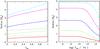 |
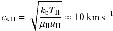
Fig. 2 Left panel: influence of the ice mass fraction fice on the radius. The reminder of the mass has a rocky composition. Radii are plotted for planets of M = 0.1 M⊕ (red solid line), 1 M⊕ (green dotted line), 10 M⊕ (blue dashed), 100 M⊕ (magenta dashed-dotted), and 1000 M⊕ (cyan short-long dashed), all without an external pressure. The thin black short-dashed-dotted line is for a 10 M⊕ core of an old 1 MX giant planet, and the thin black long-dashed-dotted line is for the 10 M⊕ core of a 10 MX giant. Right panel: radius as a function of external pressure Pext for pure ice planets. The (thick) lines represent the same planet masses as in the left panel. |
2.1.2. Core radius as function of ice mass fraction
In the left-hand panel of Fig. 2 we show the impact of the ice mass fraction in the planet fice on the radius for planets of different masses, with and without external pressure. The remainder of the mass is assumed to have a rocky composition, i.e., a 2:1 silicate-to-iron ratio.
The plot shows a planet of a mass M = 0.1 M⊕ (red solid line), 1 M⊕ (green dotted), 10 M⊕ (blue dashed), 100 M⊕ (magenta dashed-dotted), and finally for a hypothetical 1000 M⊕ solid planet (cyan short-long dashed line). All these cases were calculated without an external pressure. One can see that with increasing ice fraction, the radius increases, as expected. For most of the domain of fice, R increases about linearly with the ice fraction, which is in agreement with the results of Fortney et al. (2007).
The thin black short and long-dashed-dotted lines are, as before, for a 10 M⊕ core inside a 1 and 10 MX planet, respectively. Compared to the blue line (also 10 M⊕, but without external pressure), these lines lie at clearly smaller radii. The composition becomes less important: for Pext = 0, R increases by a factor 1.44 when going from fice = 0 to fice = 1, which is in good agreement with the fitting formula from Fortney et al. (2007) and corresponds to the result expected when the mean density of rocky material is three times higher than ice.
With the high external pressures, we find in contrast a radius increase by only a factor of about 1.19 and 1.15 for the Jovian and super-Jupiter case, respectively. This is due to the fact that for the (completely) degenerate electron gas, the density for a given pressure depends on the material only via the mean molecular weight per free electron μe (Cox & Giuli 1968). The mean molecular weight per free electron (and thus the density in the limit of complete degeneracy) of rocky material is, however, only about 1.14 times higher than the μe of pure water ice. This explains why the dependence of the radius on the specific core material becomes weaker at very high pressures.
2.1.3. Core radius as function of external pressure
In the right-hand panel of Fig. 2 we show how the radius decreases as the pressure acting on the surface of the planet increases. The external pressure is varied between the (low) pressure on the Earth’s surface and the extremely high pressure found at the core-envelope boundary of a ~20 MX planet. The lines represent the same planet masses as in the left-hand panel. A composition of 100% ice is assumed. The results for rocky material are qualitatively identical.
We see that up to a Pext of about 1010 Pa (for lower core masses) to 1012 Pa (at high core masses), the radius is independent of Pext. Such a critical pressure is roughly expected (Seager et al. 2007) because the bulk modulus of ice is of order 1010 (Benz & Asphaug 1999) to 1011 Pa (for the EOS used here, see Seager et al. 2007). After a pressure of this order is reached, the chemical bonds in the material start to get crushed, and the radius decreases. With increasing density, the pressure of the degenerate electrons becomes increasingly important.
In Sect. 5, we study the effect of a variable core density on the formation and evolution of Jupiter, while in Sect. 7.10 we look at core radii as found in a population synthesis calculation.
2.2. Uncertainties in the radius calculations
The different sources of uncertainty that affect theoretical models calculating planetary radii have been addressed in many works (e.g., Seager et al. 2007; Baraffe et al. 2008; Grasset et al. 2009). We here discuss simplifications that are specific to our model. In view of the population synthesis calculations presented below, where comparisons are made with the observed radii, it is important to estimate the uncertainties that are introduced by these simplifications. For the solid core, we have neglected the internal temperature profile and used a simple modified polytropic EOS as well as a Si/Fe ratio fixed at the terrestrial value. For the gaseous envelope, we assume that all solids reside in the core (no heavy element mixing with the envelope) and use simple gray atmospheric boundary conditions (Paper I). We next discuss the possible impact of these simplifications.
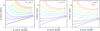 |
Fig. 3 Radii of low-mass planets with H2/He atmospheres. In all panels, the core radius is shown, and the total radius for different envelope mass fractions f, as labeled in the figures. In the left panel, thick lines show the result from this work (simple gray atmospheres), while thin lines are the results of Rogers et al. (2011) calculated with the more accurate “two-stream” approximation of Guillot (2010). Planets in the right panel have a purely rocky core, otherwise an ice mass fraction fice = 0.67 is used. The intrinsic luminosity per mass is 10-6.5 erg g-1 s-1 in all cases. The equilibrium temperature is indicated in the panels. To the right of the black dotted line, the gray atmosphere should not introduce errors larger than ~ 15% in the calculations with Teq = 250 K. |
2.2.1. Solid core
No temperature structure. Grasset et al. (2009) found that very large thermal variations within
iron-silicate planets affect the radius only on a low, ~1.5% level, in agreement with
Valencia et al. (2006). For water ice, the
thermal pressure could be more important (Fortney et al. 2007). But also for planets made of water ice, the errors in the radius
introduced by neglecting the thermal pressure are small, as it decreases the density by
typically 3% or less in the relevant domain (Seager et al. 2007). Even if the mean
density  decreased by 10%, it would cause an increase of the radius by only about 3.6%, thanks to
the weak dependency of
decreased by 10%, it would cause an increase of the radius by only about 3.6%, thanks to
the weak dependency of  .
.
Simplified EOS. As shown in Fig. 1, the simple polytropic EOS leads to radii of solid planets which agree on a 1 − 3% level for M ≲ 100 M⊕ with the results obtained when combining the Birch-Murnagham EOS, density functional theory, and a modified Thomas-Fermi-Dirac EOS (Zapolsky & Salpeter 1969). This agrees with the findings of Seager et al. (2007).
Fixed silicate-iron ratio. Grasset et al. (2009) studied in detail the effects of different [Mg/Si] and [Fe/Si] values. Using observed abundances of extrasolar host stars and assuming that the planets have the same relative abundances in Fe, Mg, and Si as their hosts, they found that the radii of rocky planets only change by less than 1.5% when the composition varies over the observed domain. Larger differences in the radii, however, occur if one abandons the assumption of identical relative abundances in planets and the host star. Such a situation can result from collisional mantel stripping, as might have occurred for Mercury (e.g., Benz et al. 2007). For a 1 M⊕ planet, Marcus et al. (2010) find a minimal plausible planetary radius achievable by maximum mantel stripping, which is about 0.85 R⊕.
As a word of caution, one must mention that most of the rather low uncertainties were estimated for low-mass planets. Baraffe et al. (2008) show that the uncertainties can become significantly larger in the case of more extreme conditions as found in the center of a giant planet. Under such conditions, they find, for example, that the density of water as predicted by various equations of state can differ by up to ~20%.
2.2.2. Gaseous envelope
All solids in the core. The consequences of how the heavy elements are distributed in a (giant) planet have been analyzed in detail by Baraffe et al. (2008). The two limiting cases are either that all solids reside in the core, surrounded by a pure H2/He envelope (as in our model), or that there is no core and the solids are uniformly mixed with the gas. For a Neptunian planet and a heavy element mass fraction Z = MZ/M of up to 20%, putting all solids in the core versus uniform mixing typically leads to a change of the radius by ~10% during the long-term evolution. For a Jovian planet with Z = 20% or 50%, the variation in the radius is of order 4% and 12%, respectively. For both planet types, putting the solids in the core leads to larger radii.
Gray atmosphere model. The Kepler satellite has recently detected large numbers of planets with radii between that of the Earth and those of the ice giants, allowing the study of the composition of such objects (Sect. 7.6). Most of these transiting planets are inside ~0.5 AU from their host star and are thus subjected to significant levels of irradiation. It is well known (e.g., Guillot & Showman 2002) that strong irradiation can significantly affect the evolution of a planet and lead to atmospheric structures more complex than the simple gray atmosphere we use (Paper I). In the current version of our model, we do not allow planets to migrate closer than 0.1 AU to the star, so that the cases undergoing the strongest effects are excluded by construction. But also at a distance of 0.1 AU, the irradiation already affects the radius of low-mass planets with H2/He atmospheres (Rogers et al. 2011). In order to estimate the uncertainty introduced by using the simple gray atmosphere model, we compare in Fig. 3 the radii of low-mass planets with H2/He atmospheres with those found by Rogers et al. (2011). These authors use a more realistic “two-stream” atmosphere (Guillot 2010). The radii shown in Fig. 3 were not found by combining formation and evolution calculations as in the rest of this study, but by directly specifying the composition of the planets, their semimajor axis, and the intrinsic luminosity (“equilibrium model” in the terminology of Rogers et al. 2011). Then, the same method as in the evolutionary calculations was used to obtain the radii. In all models, the intrinsic luminosity per mass is 10-6.5 erg g-1 s-1 as in Rogers et al. (2011). The left-hand panel shows the radii for planets with an equilibrium temperature of 500 K, which for zero albedo corresponds to an orbital distance of about 0.3 AU around a solar-like star. In this and the middle panel, a composition of the core with an ice mass fraction of 67% and 33% rocky material was assumed. This is similar, but not identical, to those in Rogers et al. (2011), because of a somewhat different composition of the silicates. The resulting radius of the core is also shown in the figure. A comparison of the thick and thin lines shows that both models lead to the same global pattern (as also found in Valencia et al. 2010). At a total mass of the planet of 20 M⊕, our model predicts total radii (i.e., τ = 2/3) that are 2% larger than those in Rogers et al. (2011), independent of the envelope mass fraction f = MXY/M = 1 − Z. This difference is partially due to an identical difference in the core radius. When moving to smaller planetary masses, the differences get larger, in particular for planets with a high envelope mass fraction. This is expected, as such low-mass, high f planets are particularly sensitive to irradiation. At M = 4 M⊕, for f = 0.05, we find radii that are 7% larger, while for f = 0.5, the difference becomes significant at about 25%. In the combined formation-evolution calculations, however, the envelope mass fraction scales with the total mass of the planet (see Fig. 10), so that low-mass planets with very massive envelopes cannot exist. This is a natural consequence of the long KH timescales of low-mass cores. At a total mass of 4 M⊕, for example, the mean f in the synthesis is approximately 0.05, and no planet has f > 0.2, where the overestimation of the radius due to the simple gray atmosphere is about 10%. Preliminary calculations also using the “two-stream” approximation lead to radii that are in excellent agreement with Rogers et al. (2011), which shows that the gray atmosphere is indeed the reason for the differences. We can thus conclude that as long as a planet is not in the regime where R is clearly increasing with decreasing mass (hot, low M, high f planets), the errors introduced by the gray atmosphere are less than ~15%. In this light, the radii in the middle and left-hand panel of Fig. 3 (equilibrium temperature of 250 K) to the right of the dotted line should not be too affected by the gray approximation.
Figure 10 shows that only a tiny fraction of the synthetic planets falls in the regime where the gray atmosphere introduces large differences, thanks to the fact that we model planets with a ≥ 0.1 AU only. We must, however, keep in mind that we have compared here equilibrium models only, i.e., we have not studied how a different atmospheric boundary condition affects the entire temporal evolution. This will be addressed in future work.
2.2.3. Summary
In summary we see that, depending on the properties of a planet, the errors affecting the radius are of a different level. A clearly gas-dominated Jovian planet at large orbital distance is less affected than a low-mass planet with a 20% H2/He atmosphere at 0.1 AU, even if we cannot reach the level of refinement for the giant planet that are attained in dedicated models for individual planets (e.g., Fortney et al. 2011).
When considering the uncertainties of the radii in a bigger context, one should keep in mind that the evolution of planets is by itself a complex problem, which is studied in dedicated evolutionary models. In the combined formation and evolution model shown here, however, the evolutionary part serves first of all to establish a link between observable properties of planets at late times, and the formation model, where many mechanisms are poorly understood. When used in planetary population synthesis calculations, the model must thus be sufficiently accurate so that possible observational findings, like e.g., correlations between radius and planet mass, host star metallicity, and semimajor axis, are not lost as constraints for the formation model. This results in different requirements than when one is interested in determining as exactly as possible the composition of one specific planet.
2.3. Core luminosity due to radioactive decay
During the accretion of planetesimals, the luminosity of the core due to this process is
approximatively  (2)where
MZ is the mass of the core,
Rcore its radius,
ṀZ the accretion rate of planetesimals,
and G the gravitational constant. This equation is applicable if the
planetesimals or their debris sink to the core (cf. Mordasini et al. 2005) and if their initial velocity is small compared to the escape
velocity of the core. In our previous models, the accretion of planetesimals is the only
source of luminosity of the core. This means that once the accretion of solids ceases,
core luminosity drops to zero. However, several processes can lead to a non-zero core
luminosity during the evolution of the core at constant mass (see Baraffe et al. 2008): the cooling of the core due to its internal
energy content dU/dt, its
contraction − PdV/dt,
and the decay of radioactive elements contained in it. Within the upgraded model, we now
take into account the last two points (see Paper I for the contraction). In the following
section we describe how we model the last mechanism.
(2)where
MZ is the mass of the core,
Rcore its radius,
ṀZ the accretion rate of planetesimals,
and G the gravitational constant. This equation is applicable if the
planetesimals or their debris sink to the core (cf. Mordasini et al. 2005) and if their initial velocity is small compared to the escape
velocity of the core. In our previous models, the accretion of planetesimals is the only
source of luminosity of the core. This means that once the accretion of solids ceases,
core luminosity drops to zero. However, several processes can lead to a non-zero core
luminosity during the evolution of the core at constant mass (see Baraffe et al. 2008): the cooling of the core due to its internal
energy content dU/dt, its
contraction − PdV/dt,
and the decay of radioactive elements contained in it. Within the upgraded model, we now
take into account the last two points (see Paper I for the contraction). In the following
section we describe how we model the last mechanism.
2.3.1. Chondritic radiogenic heating
Urey (1955) was the first to point out that the presently measured surface heat flux of the Earth roughly corresponds to the radiogenic heat released in the interior if the Earth has a chondritic composition. This observation still holds today, even though the details depend on the exact type of chondritic material that is assumed to have formed the Earth (Hofmeister & Criss 2005). Estimates for the total flux vary, but are of order 3 × 10²⁰ erg/s (Hofmeister & Criss 2005). Due to these findings, we model the radiogenic heat production as the consequence of the decay of the three most important long-lived nuclides 40K, 238U, and 232Th (Wasserburg et al. 1964), assuming a chondritic composition. We further assume that the radiogenic heat production rate in the interior and the loss at the surface are in equilibrium, i.e., the luminosity at the surface is equal to the instantaneous radiogenic energy production rate inside the planet. We therefore neglect a possible delayed secular cooling and possible residual heat from the impacts during the formation of the planet. This is, at least for Earth today, a good approximation (Hofmeister & Criss 2005).
As illustrated below, the radiogenic luminosity Lradio obtained this way is small, but not negligible, for the total luminosity of low-mass (super-Earth) planets with a tenuous H2/He atmosphere, i.e., Lradio provides a physically motivated minimum for the luminosity of the core, once the accretion of planetesimals has ceased. This can play a role in the evolution of the total radius, which is an observable quantity, as demonstrated in Sect. 6.
Valencia et al. (2010) simply use a total heat
production rate of
2 × 10²⁰ erg s-1  for the planet’s mantel, which is also assumed to have a chondritic composition. They
assume that the rate is constant in time. We improve this by considering that over
timescales of billions of years heat production by long-lived radionuclides will
decrease according to the law of exponential radioactive decay.
for the planet’s mantel, which is also assumed to have a chondritic composition. They
assume that the rate is constant in time. We improve this by considering that over
timescales of billions of years heat production by long-lived radionuclides will
decrease according to the law of exponential radioactive decay.
Denoting with Q(t) the energy release per second per
gram of chondritic material, one can write (e.g., Prialnik et al. 1987)  (3)where
Q0 is the heat production rate per gram of chondritic
material at time t = 0 and
λ = ln2/t1/2
is the decay constant for a radionuclide with a
half-life t1/2. The values
of Q0 can be found by extrapolating back from currently
measured values in meteorites. In Table 1, we
give the values of λ and Q0 derived from
the data given in Lowrie (2007) for the three
nuclides we include. These values are compatible with the ones of Prialnik et al. (1987).
(3)where
Q0 is the heat production rate per gram of chondritic
material at time t = 0 and
λ = ln2/t1/2
is the decay constant for a radionuclide with a
half-life t1/2. The values
of Q0 can be found by extrapolating back from currently
measured values in meteorites. In Table 1, we
give the values of λ and Q0 derived from
the data given in Lowrie (2007) for the three
nuclides we include. These values are compatible with the ones of Prialnik et al. (1987).
Parameters for the radiogenic heat production.
The total heating rate per gram of chondritic material is then simply
 (4)In Fig. 4, we plot Qtot and the
contribution of the three nuclides as a function of time. Initially, potassium provides
the dominant contribution, by about an order of magnitude. At later
times, 238U and 232Th take over due to their longer half-life.
(4)In Fig. 4, we plot Qtot and the
contribution of the three nuclides as a function of time. Initially, potassium provides
the dominant contribution, by about an order of magnitude. At later
times, 238U and 232Th take over due to their longer half-life.
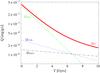 |
Fig. 4 Radiogenic heat production rate in one gram of chondritic material as a function of time due to the decay of long-living nuclides. The lines show the contribution from the different radionuclides (as labeled in the figure), as well as the total rate (red solid line). |
The total radioactive luminosity of the core is given as  (5)where
MZ is the total core mass,
fmantle the mantle fraction, and
frocky = 1 − fice the mass
fraction of rocky material in the core.
(5)where
MZ is the total core mass,
fmantle the mantle fraction, and
frocky = 1 − fice the mass
fraction of rocky material in the core.
With this setting, one finds for an Earth-like planet (fmantle = 2/3, frocky = 1, MZ = 1 M⊕) at t = 4.5 Gyr a radioactive luminosity of Lradio = 2.26 × 10²⁰ erg/s, which is in good agreement with the value from Valencia et al. (2009). For t = 0, one finds Lradio = 1.65 × 10²¹ erg/s, or about a factor 7.3 higher than today. This is in good agreement with Wasserburg et al. (1964), who estimate a ratio of 4.5 to 8.2, depending on the chemical composition of the Earth. In a similar approach, Nettelmann et al. (2011) find a present time radiogenic heat production rate of 2.3 × 10²⁰ erg/s and a value of 2.7 × 10²¹ erg/s at t = 0. The latter value is higher than found here, probably because we have not included 235U due to its relatively short half-life of 0.47 Gyr. The value of the radiogenic luminosity due to long-lived nuclides at t = 0 (or up to small t ~ 10 Myr, Prialnik et al. 1987) has no practical meaning, as short-lived radionuclides and heat produced by collisional growth would then dominate by many orders of magnitude. It gives, however, an impression by how much the heat flux has varied over the lifetime of the solar system due to long-lived radionuclides.
2.3.2. Short-lived radionuclides
We have neglected radiogenic heating due to short-lived radionuclides, in particular aluminium 26. It is well known that 26Al could have been a powerful heating mechanism in the first few million years in the solar system (e.g., Prialnik et al. 1987). According to the study of Castillo-Rogez et al. (2009), who assume an initial isotopic abundance ratio of 26Al/27Al = 5 × 10⁻⁵, an aluminium concentration of 1.2 wt % in silicates, one finds a Q0,Al = 2.13 × 10⁻³ erg/(g s). This value is compatible with the one given in Prialnik et al. (1987). This is many orders of magnitude more than for the long-lived nuclides. If we were to have a fully assembled rocky 1 M⊕ planet at t = 0, then 26Al would lead to a luminosity of about 2.5 LX and a surface temperature of 414 K (neglecting melting and a delayed heat transport, which is clearly not realistic in this case).
It is difficult to derive a general model (i.e., for stars other than the sun) that includes short-lived radionuclides for a number of reasons. First, it is unclear how universal the initial abundance of short-lived radionuclides is for different planetary systems. If non-local effects play an important role (like the proposed nearby supernova, Cameron & Truran 1977), then we probably must expect very different initial concentrations. Second, due to the short half-life of 26Al (about 0.72 Myr), results regarding this nuclide are very sensitive to the exact time delay between CAI formation and inclusion into the planetesimals and protoplanets (e.g., Prialnik et al. 1987). The time corresponding to t = 0 is not very well defined in our simulations. For example, the distribution of initial disk masses is based on observations of YSO in ρ Ophiuchi, which is about 1 Myr old (Andrews et al. 2009). Third, the inclusion of short-lived nuclides would require a detailed thermic model of the core, allowing melting and heat transport. This is currently beyond the scope of the model. The same applies to heating due to impacts.
In Sect. 6, we illustrate the effect of radiogenic heat production on the luminosity of a low-mass planet with a tenuous primordial H2/He atmosphere.
3. Disk model
We next turn to three improvements of the model of the protoplanetary disk. The properties of the protoplanetary disk are the initial and boundary conditions for the growth and migration of the planets. The disk model yields, for example, the outer boundary conditions for the structure equations, the radial slopes of the temperature, and the surface density for the migration model as well as the gas accretion rate in the runaway phase (cf. Alibert et al. 2005 and Paper I). In this computational module, we have improved the initial conditions for the disk evolution, the description of photoevaporation, and the treatment of the outer and inner disk edge.
3.1. Standard α model with irradiation and photoevaporation
As in previous studies, we solve the standard equation for the evolution of the surface density of a viscous accretion disk (Lynden-Bell & Pringle 1974) in a 1+1D model (vertical and radial structure), assuming that the viscosity can be calculated with the α approximation (Shakura & Sunyaev 1973).
A detailed description of the disk model, especially how the vertical structure is calculated assuming an equilibrium of viscous heating and radiation at the surface, was given in Alibert et al. (2005). In Fouchet et al. (2012), we have shown how we take into account heating by stellar irradiation, assuming that the flaring angle is at the equilibrium value of 9/7 (Chiang & Goldreich 1997).
In previous studies, we used an initial gas surface density profile inspired by the
minimum mass solar nebula (Weidenschilling 1977;
Hayashi 1981), which is given as  (6)at
a distance r from the star. Here, Σ0 is the initial gas
surface density at our reference distance R0 = 5.2 AU. We also
used a fixed outer radius of the disk of 30 AU. In the updated model, the disk is free to
spread or shrink at the outer edge, and the initial gas surface density profile takes
the form
(6)at
a distance r from the star. Here, Σ0 is the initial gas
surface density at our reference distance R0 = 5.2 AU. We also
used a fixed outer radius of the disk of 30 AU. In the updated model, the disk is free to
spread or shrink at the outer edge, and the initial gas surface density profile takes
the form ![Mathematical equation: \begin{equation} \Sigma(r,t=0)=\Sigma_0\left(\frac{r}{R_0}\right)^{-\gamma}\exp\left[-\left(\frac{r}{R_{\rm c}}\right)^{2-\gamma}\right], \label{eq:newprofilegeneral} \end{equation}](/articles/aa/full_html/2012/11/aa18464-11/aa18464-11-eq126.png) (7)which corresponds to a
power-law for radii much less than Rc, followed by an
exponential decrease. As shown by Andrews et al. (2009), this form can be derived from the similarity solution of the viscous disk
problem of Lynden-Bell & Pringle (1974).
We use two radii, R0 and Rc,
instead of only Rc. This does not mean that we introduce an
additional parameter; it just means that the normalization constant Σ0 takes
another value, namely, the one at 5.2 AU, which simplifies comparison with previous work.
Andrews et al. (2009, 2010) note that profiles with an exponential decrease provide better
agreement with observations than a pure power-law profile with a sharp outer edge. The
observed values for γ roughly follow a normal distribution with a mean of
γ = 0.9 and a standard deviation of 0.2, which is compatible with one
uniform value characterizing the entire observational sample of 16 disks (Andrews et al.
2010). We therefore use γ = 0.9
in the simulations (see Appendix A).
(7)which corresponds to a
power-law for radii much less than Rc, followed by an
exponential decrease. As shown by Andrews et al. (2009), this form can be derived from the similarity solution of the viscous disk
problem of Lynden-Bell & Pringle (1974).
We use two radii, R0 and Rc,
instead of only Rc. This does not mean that we introduce an
additional parameter; it just means that the normalization constant Σ0 takes
another value, namely, the one at 5.2 AU, which simplifies comparison with previous work.
Andrews et al. (2009, 2010) note that profiles with an exponential decrease provide better
agreement with observations than a pure power-law profile with a sharp outer edge. The
observed values for γ roughly follow a normal distribution with a mean of
γ = 0.9 and a standard deviation of 0.2, which is compatible with one
uniform value characterizing the entire observational sample of 16 disks (Andrews et al.
2010). We therefore use γ = 0.9
in the simulations (see Appendix A).
3.2. Stability against self-gravity
In order to check whether we specify initial conditions that make the application of our (constant) α model self-consistent, we take a look at which disks with the new initial profile are stable against the development of spiral waves due to self-gravity.
The sound speed cs is given as
 (8)where
Tmid is the midplane temperature (obtained from our vertical
structure model), μ the mean molecular weight (set to 2.27),
kb the Boltzmann constant,
and mH the mass of a hydrogen atom. The Keplerian
frequency Ω at a distance r around a star of
mass M∗ is given as
(8)where
Tmid is the midplane temperature (obtained from our vertical
structure model), μ the mean molecular weight (set to 2.27),
kb the Boltzmann constant,
and mH the mass of a hydrogen atom. The Keplerian
frequency Ω at a distance r around a star of
mass M∗ is given as
 (9)and the Toomre (1981) parameter is given as
  (10)assuming that the
disk is in Keplerian rotation despite its own mass.
(10)assuming that the
disk is in Keplerian rotation despite its own mass.
With a Toomre QToomre smaller than unity, the disk is unstable against local axisymmetric (ring-like) gravitational disturbances. Numerical simulations show that non-axisymmetric disturbances (multi-armed spiral waves) start growing slightly earlier at QToomre,crit ≲ 1.7 (Durisen et al. 2010).
For massive disks (Mdisk/M∗ ≳ 0.1), one has to consider global instabilities, too. In particular, the m = 1 mode (corresponding to a one-armed spiral) was initially thought to be crucial (Adams et al. 1989; Shu et al. 1990) as it can be amplified by the SLING mechanism. It should, however, be noted (cf. Bodenheimer 1992; Papaloizou & Lin 1995) that the type of instability described by Adams et al. (1989) and Shu et al. (1990) is sensitive to the outer boundary condition of the disk as it requires a sharp outer edge in order to reflect incoming density waves. This is not the case for the disk profile considered here, and the nonlinear numerical simulations of Christodoulu & Narayan (1992) and Heemskerk et al. (1992) have not confirmed this specific type of instability. Later numerical simulations have found (e.g., Nelson et al. 1998; Lodato & Rice 2004) that lower (global) modes become more important with increasing disk mass, but have a mixed character involving various modes with m ≲ 5. We address the global stability in Appendix A.3.
3.3. Stability against clumping
If QToomre ≲ 1.7, spiral arms develop in the disk. Another question is whether these arms can fragment into bound clumps of self-gravitating gas. This question can be addressed by looking at the cooling timescale.
The representative gas density ρ in the disk is given as
 ,
where H is the vertical scale height, while the optical
depth τ is approximatively
τ = κ(ρ,Tmid)Σ/2,
where κ is the opacity taken from Bell & Lin (1994) and Σ is the local gas surface density. The
effective optical depth can be estimated as
,
where H is the vertical scale height, while the optical
depth τ is approximatively
τ = κ(ρ,Tmid)Σ/2,
where κ is the opacity taken from Bell & Lin (1994) and Σ is the local gas surface density. The
effective optical depth can be estimated as  (Rafikov
2005), so that the cooling
timescale τcool of a gas parcel is approximatively (Kratter
et al. 2010)
(Rafikov
2005), so that the cooling
timescale τcool of a gas parcel is approximatively (Kratter
et al. 2010)
 (11)This expression is valid
both in disks where irradiation or viscous dissipation is the main heating source, modulo
order unity factors. For simplicity, we have assumed that the adiabatic index of the gas
is γad = 7/5 everywhere. Strictly speaking,
this is appropriate only in the colder parts of the disk where hydrogen is molecular.
(11)This expression is valid
both in disks where irradiation or viscous dissipation is the main heating source, modulo
order unity factors. For simplicity, we have assumed that the adiabatic index of the gas
is γad = 7/5 everywhere. Strictly speaking,
this is appropriate only in the colder parts of the disk where hydrogen is molecular.
In order to form a bound clump, and prevent it from being sheared apart, the clump must
cool on a timescale comparable to the orbital timescale, or in other words (Gammie 2001)
 (12)where we assume a
critical ξ = 3 (Kratter et al. 2010). In the Appendix A, we use these equations to determine the most massive
stable disk, and to study the general stability of irradiated α disks.
(12)where we assume a
critical ξ = 3 (Kratter et al. 2010). In the Appendix A, we use these equations to determine the most massive
stable disk, and to study the general stability of irradiated α disks.
3.4. Photoevaporation
In the first generation of the model (Alibert et al. 2005), we calculated the mass loss of the disk due to photoevaporation
according to  (13)where
we set the gravitational radius Rg equal 5 AU, and
Rmax = 30 AU was the total radius in the old model. In this
prescription, the mass loss is concentrated at Rg (similar to
internal photoevaporation), but the total loss rate was externally specified, similar to
external photoevaporation.
(13)where
we set the gravitational radius Rg equal 5 AU, and
Rmax = 30 AU was the total radius in the old model. In this
prescription, the mass loss is concentrated at Rg (similar to
internal photoevaporation), but the total loss rate was externally specified, similar to
external photoevaporation.
It should be noted that the primary role of photoevaporation in the framework of planet formation models like the one here is to act as a controlling mechanism for the disk lifetime, which is important for the final mass of giant planets. A more precise description of photoevaporation (especially where how much gas is removed) is in contrast not very important, as the detailed description is important only when the typical disk surface density (or alternatively, the accretion rate onto the star) has become small. At such surface densities, the main gas-driven mechanisms (gas accretion, tidal migration) have, however, already fallen to a low level.
3.5. External photoevaporation
In the updated model, we split the mass loss due to photoevaporation into two components: external photoevaporation due to the presence of massive stars in the birth cluster of the host star and internal photoevaporation by the planet’s host star itself.
For external photoevaporation, we follow the description of far-ultraviolet (FUV)
evaporation in Matsuyama et al. (2003). The
FUV radiation (6−13.6 eV) heats a neutral layer of dissociated hydrogen (mean molecular
weight μI = 1.35) to a temperature of order
TI = 103 K, which launches a supersonic flow. We
thus get a sound speed  (14)and
a gravitational radius
(14)and
a gravitational radius  (15)which corresponds
to about 144 AU for a 1 M⊙ star. Following Matsuyama et al.
(2003), we assume that mass is removed outside
the effective gravitational
radius βIRg,I
with βI = 0.5 and that the total mass loss rate is
(15)which corresponds
to about 144 AU for a 1 M⊙ star. Following Matsuyama et al.
(2003), we assume that mass is removed outside
the effective gravitational
radius βIRg,I
with βI = 0.5 and that the total mass loss rate is
 (16)where
Ṁwind,ext is a parameter that gives the
total mass loss rate if the disk has an outer radius of
Rmax = 1000 AU. The effect of this mechanism is thus to remove
mass outside a radius of about 70 AU. In practice, it is found that the actual total mass
loss rates are clearly smaller than the
specified Ṁwind,ext because the disk
evolves to a state where the outer radius is given by the equilibrium of mass removal by
photoevaporation, and outward viscous spreading (see also Adams et al. 2004).
(16)where
Ṁwind,ext is a parameter that gives the
total mass loss rate if the disk has an outer radius of
Rmax = 1000 AU. The effect of this mechanism is thus to remove
mass outside a radius of about 70 AU. In practice, it is found that the actual total mass
loss rates are clearly smaller than the
specified Ṁwind,ext because the disk
evolves to a state where the outer radius is given by the equilibrium of mass removal by
photoevaporation, and outward viscous spreading (see also Adams et al. 2004).
In this description of external photoevaporation, we have not taken into account that if the host star is born in a large cluster with OB stars and the distance to one of the massive stars is small (d ≲ 0.03 pc for the Trapezium Cluster, Johnstone et al. 1998), ionizing extreme-ultraviolet (EUV) radiation can lead to a very rapid dispersal of the protoplanetary disk (Matsuyama et al. 2003). It is, however, unlikely that such a very high radiation environment is representative for the majority of young stars we are interested in here (Adams et al. 2004; Roccatagliata et al. 2011 for an observational study). We have also neglected the findings of Adams et al. (2004) that significant mass loss due to external FUV radiation might also happen well inside Rg,I, leaving this for consideration in further work.
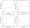 |
Fig. 5 Effect of variable core density on the in situ formation and evolution of Jupiter. In each panel, red solid lines show the case of a variable core density, while blue dotted lines correspond to a constant core density of 3.2 g/cm3. The top left panel shows the core mass as a function of time during the formation phase; afterwards it is constant. The top right panel is the radius of the core. The local maximum for the variable density case occurs at about 1 Myr. The bottom left panel is the mean core density. The bottom right panel finally shows the total radius of the planet during the long-term evolution. |
3.6. Internal photoevaporation
The photoevaporation due to the host star is modeled as in Clarke et al. (2001), which is based on the “weak stellar wind” case
studied by Hollenbach et al. (1994). In this model,
the EUV radiation (
>13.6 eV) from the host star leads to an
ionized layer with a temperature of order
TII = 104 K, where the mean molecular mass is
μII = 0.68. The sound speed is then
 (17)and
the gravitational radius is
(17)and
the gravitational radius is 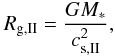 (18)which corresponds
to about 7 AU for a 1 M⊙ star. Like Clarke et al. (2001), we use a scaling radius
R14 = βIIRg,II/1014 cm
and assume a βII = 0.69, which means that the effective
gravitational radius is located at 5 AU as in our earlier models. The base density can be
estimated as
(18)which corresponds
to about 7 AU for a 1 M⊙ star. Like Clarke et al. (2001), we use a scaling radius
R14 = βIIRg,II/1014 cm
and assume a βII = 0.69, which means that the effective
gravitational radius is located at 5 AU as in our earlier models. The base density can be
estimated as 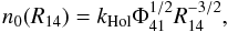 (19)where the constant
kHol = 5.7 × 10⁷ is taken from the hydrodynamic
simulations by Hollenbach et al. (1994)
and Φ41 is the ionizing photon luminosity of the central star in units of
1041 s-1. We assume Φ41 = 1. The base density varies
with radius as
(19)where the constant
kHol = 5.7 × 10⁷ is taken from the hydrodynamic
simulations by Hollenbach et al. (1994)
and Φ41 is the ionizing photon luminosity of the central star in units of
1041 s-1. We assume Φ41 = 1. The base density varies
with radius as  (20)which means that most of
the wind is originating close to the effective gravitational radius. The decrease of the
surface density is then finally
(20)which means that most of
the wind is originating close to the effective gravitational radius. The decrease of the
surface density is then finally  (21)This
results in a total constant mass loss rate due to internal photoevaporation of about
3 × 10⁻¹⁰ M⊙/yr, a value similar to what
was found by Alexander & Armitage (2009).
(21)This
results in a total constant mass loss rate due to internal photoevaporation of about
3 × 10⁻¹⁰ M⊙/yr, a value similar to what
was found by Alexander & Armitage (2009).
The final photoevaporation rate that enters the master equation for the evolution of the
surface density (see, e.g., Alibert et al. 2005) is
then given by the sum of the two mechanisms
 (22)The
characteristic evolution of a protoplanetary disk under the influence of the
photoevaporation model presented here has essentially already been shown in Clarke et al.
(2001) and Matsuyama et al. (2003). To allow comparison and for reference, we show
our results regarding the protoplanetary disk model in Appendices A and B.
(22)The
characteristic evolution of a protoplanetary disk under the influence of the
photoevaporation model presented here has essentially already been shown in Clarke et al.
(2001) and Matsuyama et al. (2003). To allow comparison and for reference, we show
our results regarding the protoplanetary disk model in Appendices A and B.
4. Results
We use the upgrades of the model to study first the effect of the variable core density on the in situ formation and evolution of Jupiter (Sect. 5). In Sect. 6, we then analyze the evolution (and formation) of a close-in super-Earth planet for which the radiogenic heating of the core influences the evolution of the radius, which is potentially relevant for transit observations. We also compare our results with previous studies. The most important result is shown in Sect. 7 where we study the formation and evolution of the planetary M − R relationship with population synthesis calculations. We compare the synthetic M − R relationship with the observed one and derive an expression for the mean planetary radius as function of mass. Comparisons are also made with the radius distribution as found by the Kepler satellite.
5. Jupiter formation and evolution: effect of a variable core density
Figure 5 compares the in situ formation and evolution with a constant core density of 3.2 g/cm3 (as usually assumed in formation models, e.g., Pollack et al. 1996; or Movshovitz et al. 2010) and a variable one, using the model described above. The simulation with a variable core density is the nominal case discussed in Paper I, where all parameters used in the simulation can be found. Except for the density, all settings are identical in the two simulations.
The top left-hand panel of the figure shows the core mass as a function of time during the formation phase. It immediately demonstrates that the formation is very similar in both cases, in agreement with Pollack et al. (1996), who found only a weak dependence of the formation on the core density. The core grows in the simulation with the constant density during phase I initially slightly slower, since the actual mean density is still smaller (about 2 g/cm3), as can be seen in the bottom left-hand panel. This leads to a larger capture radius for planetesimals and thus to faster growth. This is because in phase I, capture and core radius are initially identical (Paper I).
For the variable density, the growth of the core leads to an increase of the density due to the increasing pressure; as a result, the two densities become equal roughly in the middle of phase I. From now on, the actual density is always larger than 3.2 g/cm3. Further mass accretion in phase II is similar in both cases. This is because the capture radius for planetesimals is now between 10 to 60 times larger than Rcore. The capture radius is similar in both cases because the density structure in the envelope relevant for the capture is also similar in both cases, being located quite far away from the core. The mean core density in phase II is of order 4 g/cm3, i.e., quite close to the constant value. As the runaway gas accretion phase is approached, the density in the variable case increases; as a result, the evolution starts to diverge slightly, with the constant density case growing faster. This leads to a difference in the formation timescale of somewhat less than 105 years, corresponding to about 10%.
The collapse of the planet and the rapid accretion of ~300 Earth masses of gas lead to a rapid increase of the core density during the collapse/gas runaway accretion phase, due to the quickly growing external pressure exerted on the core. The density goes up rapidly from about 5 to 10 g/cm3. The core grows during the same time by another ~17 M⊕ in mass. The increase of the density, however, over-compensates that, so that Rcore actually shrinks after having reached a local maximum, as visible in the top right-hand panel. This is an interesting effect. Nevertheless, we should keep in mind that it is unclear whether the planetesimals still penetrate to the core in this phase (Paper I). The moment of the maximum core radius might have occurred at an earlier time than shown here, where it coincides with the onset of gas runaway accretion.
During the long-term evolution, a core density of 3.2 g/cm3 is clearly not realistic. The actual core densities range between 10 and 15 g/cm3 (14.3 g/cm3 at 4.6 Gyr), leading at late times to a significant difference of Rcore of about 0.13 RX between the two cases.
 |
Fig. 6 Temporal evolution of the luminosity and the radius of a close-in, super-Earth planet with a tenuous H2/He envelope (MZ = 4.2 M⊕, MXY = 0.045 M⊕, i.e., about 1%). Left panel: intrinsic luminosity as a function of time. The red solid line is the total intrinsic luminosity, while the blue dotted line is Lradio. The left axis gives L in units of present-day intrinsic Jovian luminosities. The right panel shows the total radius (red solid line) and the radius of the solid core (blue dotted line). The inset figure shows the total radius at late times. Note the delayed contraction between about 0.2 and 2 Gyr due to radiogenic heating. Atmospheric mass loss and outgassing are neglected, so that one directly sees the effect of Lradio. These simplifications could, however, also mean that the evolution is in reality more complex than shown here. |
It is interesting to investigate how this difference affects the observable total radius. This is shown in the bottom right-hand panel of Fig. 5. We find that the total radius is larger in the constant density case, too. As expected, the difference is smaller than for the core radius, namely, about 0.06 RX at 4.6 Gyr. This is clearly a non-negligible difference, as it would otherwise correspond to a difference of the core mass of about 30 M⊕ (Paper I; Fortney et al. 2007), which is a significant quantity. For accurate comparisons of our population synthesis calculations with transit observations, we must therefore include a realistic core density model, as can implicitly be deduced from the results of Fortney et al. (2007).
6. Evolution of a super-Earth planet including radioactive luminosity
In Fig. 6, we illustrate the effect of Lradio on the total luminosity of a low-mass, super-Earth planet (core mass MZ = 4.2 M⊕) that has, at the end of formation, a tenuous H2/He envelope with a mass of about MXY = 0.045 M⊕, i.e., about 1%. For comparison, Venus has an atmosphere with a mass of approximately 8 × 10⁻⁵ M⊕, which is a factor ≈ 560 less. On this scale, MXY = 0.045 M⊕ still corresponds to a relatively massive envelope.
The H2/He envelope mass of low-mass planets at the end of formation varies as it depends on a number of factors. Important quantities are the grain opacity in the envelope (see the dedicated work of Mordasini et al. 2012c), the luminosity of the core due to the accretion of planetesimals, and also, as tests have shown, the radiogenic luminosity of the core due to the decay of 26Al. Large radiogenic core luminosities during the nebular phase can lead to lower envelope masses because of a stronger pressure support in the gas at a higher temperature. By modifying the final envelope mass, short-lived radionuclides can thus have an impact on the long-term evolution of a planet in an indirect way. The planets that are most affected by this mechanism are low-mass, core-dominated rocky planets, which undergo towards the end of their formation a phase where the accretion rate of planetesimals is low. This can, for example, occur if a planet is caught in a type I convergence zone and has emptied its feeding zone. If this happens early enough compared to the half-life of the radionuclides, the radiogenic heating will reduce the amount of gas that can be accreted.
In the light of the discoveries of the Kepler satellite of a number of low-mass, low-density planets (e.g., the Kepler-11 system, Lissauer et al. 2011a) the problem of possible primordial envelope masses in the transition regime between terrestrial and water planets (without primordial envelopes) and mini-Neptunes (with primordial envelopes) has become an important one. We show our results concerning this question in Sect. 7.6.
The left-hand panel of Fig. 6 shows the total intrinsic and radiogenic luminosity (neglecting 26Al) as a function of time. During the formation of the planet, the luminosity is high, mostly due to the accretion of solids. The specific shape of L in this phase with some wave-like patterns is a consequence of the complex migration behavior of this planet, giving origin to phases with high and low planetesimal accretion rates, and thus core luminosities. The planet eventually migrates to ~0.1 AU. At about 4 Myr, the accretion of solids (and of gas) ceases. The luminosity is now dominated by the contraction and cooling of the gaseous envelope. At about 400 Myr, however, Lradio becomes the dominant source of luminosity for this planet, giving rise to a transient plateau phase of roughly constant L. Finally, beyond a few billion years, L starts to decrease again, following now the decrease of Lradio according to the radioactive decay law. As found by Nettelmann et al. (2011), we see that it is important to include radiogenic heating to accurately model the thermal evolution of core-dominated planets.
6.1. Radius evolution and comparison with Rogers et al. (2011)
Knowing the intrinsic luminosity (as well as the irradiation from the host star), we can calculate the radius of a (low-mass) planet as a function of time and thus compare it with results of transit observations. Figure 6 shows the core and total radius as a function of time. During the attached phase, the planet has a large radius (Paper I), and then contracts rapidly after accretion has stopped (i.e., when the protoplanetary gas disk disappears) to a radius of initially about 3.5 R⊕. During the following evolution, it slowly contracts to a radius of about 2.2 R⊕ at 4.6 Gyr. The core radius is only 1.46 R⊕, so despite the fact that the envelope just contains about 1% of the total mass, it contributes significantly to the radius. This is a well-known effect (e.g., Valencia et al. 2010; Sect. 2.2.2).
At an orbital distance of 0.1 AU from a solar-like star and the assumed albedo (Paper I), we get a surface temperature of the planet during the evolutionary phase of about 790 K. This temperature is virtually constant, as the contribution of the intrinsic luminosity compared to the contribution from stellar irradiation is negligible. The temporal variation of the stellar luminosity itself is currently not considered in the model. In Fig. 7, we show the temporal evolution of the pressure-temperature profile in the planetary envelope. The entire envelope is shown, so that the lower ends of the lines correspond to the temperature and pressure at the interface with the solid core. The first profile, which corresponds to the rightmost line, is shown at an age of the planet of 5 Myr, which is about one million years after the end of the formation phase. At this early time, the temperature at the core-envelope boundary is approximately 6700 K. The last profile, which is the leftmost line, shows the state at a hypothetical age of 16 Gyr. The temperature at the core-envelope interface has then fallen to ~1500 K. The intrinsic luminosity is decreasing with time, so that the envelope becomes completely radiative at an age of about 7 Gyr. At even later times, the envelope would become isothermal. Between an age of 5 Myr and 16 Gyr, additional p − T structures are shown at irregular time intervals of a few 104 yrs (at the beginning) to several 109 yrs towards the end, reflecting the increase of the numerical time step due to the increase of the Kelvin-Helmholtz timescale of the planet.
We note that our treatment of the effect of stellar irradiation on the envelope structure is very basic at the moment (Paper I) and will be improved in future (Guillot 2010; Heng et al. 2011). It is therefore likely that the upper part of the atmosphere structure is clearly more complex than shown here.
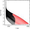 |
Fig. 7 Evolutionary sequence of the p − T structure of the envelope. The first structure (rightmost line) is at 5 Myr, the last structure (leftmost line) is at a hypothetical age of 16 Gyr. The entire internal structure is shown, which means that the lower end of a line corresponds to the core-envelope interface, while the top end corresponds to the τ = 2/3 surface. Red indicates convective parts, black radiative layers. The actual upper part of the envelope/atmosphere will be more complex than shown here, since we only use a simple gray atmosphere in the current model. |
It is interesting to compare our results with the ones of Rogers et al. (2011), who use a more realistic “two-stream” atmosphere (Guillot 2010). For a 4 M⊕ planet with a 1% envelope, these authors find a radius of about 2.7 and 3.3 R⊕, at an equilibrium temperature of 500 and 1000 K, respectively, and an intrinsic luminosity-to-mass ratio of L/M = 10-6.5 = 3.2 × 10⁻⁷ erg/(g s). These authors do not follow the temporal evolution of the internal luminosity and thus use the L/M ratio as an age proxy, as was also used to calculate Fig. 3.
Our planet has L/M ratios of 6.6 × 10⁻⁶, 5.2 × 10⁻⁷, 1.7 × 10⁻⁷, and 1.1 × 10⁻⁸ erg/(g s) at 0.01, 0.1, 1, and 10 Gyr, respectively. The values at 1 and 10 Gyr simply correspond to Eq. (5). One notes the effect of the plateau phase because of radiogenic heating between roughly 0.2 and 2 Gyr. This is also directly visible in the evolution of the radius (Fig. 6, right-hand panel), where the contraction is slowed down during this time interval. At the L/M ratio used by Rogers et al. (2011), we find a total radius of about 2.34 R⊕. A lower radius than in Rogers et al. (2011) is expected, since these authors assume an icy composition of the core resulting in a core radius of about 1.9 R⊕, while we use an Earth-like rocky composition because the planet has accreted only inside the ice line, leading to a Rcore = 1.46 R⊕. Therefore, there is a difference of the core radii of about 0.45 R⊕. Taking this into account, we see that for the total radius, the models agree on a 0.2 R⊕ or better level, corresponding to about ~7%. The comparison here and in Sect. 2.2.2 shows that the radii of low-mass super-Earth planets can be simulated for the population synthesis with relatively good accuracy.
Since the evaporation of the primordial H2/He envelope, the thermal cooling of the core, and the outgassing of a secondary atmosphere during the long-term evolution are not included, we must nevertheless keep in mind that the evolution of the planet on Gyr could in reality be more complex than shown here. Our interest was to show the differential effect of Lradio. To quantify the importance of subsequent H2 outgassing, we can use the work of Rogers et al. (2011). These authors find that a rocky planet with a composition such as we assume (2:1 silicate-to-iron ratio) could outgas H2 corresponding to about 0.2 wt% of its mass. This corresponds in the case here to 0.0084 M⊕. This is a factor ~5 less than the mass of the primordial atmosphere, so that at least this effect should not completely change the evolution.
7. Formation and evolution of the planetary M – R relationship
We now turn to the most important results of this paper. We use the upgraded model to conduct planetary population synthesis calculations and study the formation and evolution of the planetary M − R relationship. We also discuss the synthetic radius distribution and compare it with observations.
7.1. Population synthesis
The population synthesis calculations presented here are obtained with the same basic approach as introduced in Mordasini et al. (2009a). However, instead of the original formation model presented first in Alibert et al. (2004), we use the extended model described in Paper I and this work.
Table 2 lists the most important parameters for the calculations. With respect to the gas disk model, we use the new initial disk profile introduced in Sect. 3.1 (see Eq. (A.1)) with an inner border of the computational disk at 0.1 AU. We assume that the gas surface density falls to zero at this point (see Fig. B.1). We apply the new description of photoevaporation from Sect. 3.4 and use stellar irradiation (Fouchet et al. 2012) as well as viscous heating to calculate the vertical temperature structure of the disk. As in earlier works (Mordasini et al. 2009a), we fix the α viscosity parameter to 7 × 10⁻³.
Parameters and settings for the population synthesis.
Regarding the planetary seed, we start with an embryo of 0.6 M⊕. This setting and the fact that we do not calculate any planetary growth once that the gaseous disk is gone means that our model lacks an essential phase (giant impacts) in the formation of low-mass (terrestrial) planets, so that results about low-mass planets (M ≲ 10 M⊕) must be regarded with caution (see extended discussion in Mordasini et al. 2009a). For the internal structure of the core, we use the model presented in Sect. 2.1. Radiogenic heating is included as a source of core luminosity, as described in Sect. 2.3. The fraction of ice in the core is known as we keep track of how many solids are accreted inside or outside of the iceline. The position of the iceline is given by the initial temperature structure of the nebula (Mordasini et al. 2009a).
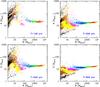 |
Fig. 8 Temporal evolution of the planetary M − R diagram during the formation phase. The colors show the fraction of heavy elements Z = MZ/M in a planet. Orange: Z ≤ 1%. Red: 1 < Z ≤ 5%. Green: 5 < Z ≤ 20%. Blue: 20 < Z ≤ 40%. Cyan: 40 < Z ≤ 60%. Magenta: 60 < Z ≤ 80%. Yellow: 80 < Z ≤ 95%. Brown: 95 < Z ≤ 99%. Black: Z > 99%. |
Only primordial H2/He envelopes are considered in the model. For the treatment of the accretion shock occurring during gas runaway accretion, we assume that the shock radiates all liberated energy, i.e., we assume a “cold start” scenario (Paper I). The gas accretion rate in the runaway phase is calculated as described in Paper I, allowing for non-equilibrium fluxes in the disk. We use the simplification of a constant luminosity within the envelope for reasons explained in Paper I. We assume that the grain opacity in the gaseous envelope is 0.003 times the value in the interstellar medium. This value has been determined in Mordasini et al. (2012c) by comparison with detailed grain evolution calculations in protoplanetary envelopes (Movshovitz et al. 2010). The tables of Freedman et al. (2008) are used for the opacity due to the grain-free gas. Two effects related to the planetary envelope, which can be relevant during the long-term evolution of the planet, are currently not included. First, we do not include deuterium burning in the low number of planets that grow beyond the D-burning limit. This will affect the radius of objects more massive than ~13 MX at early times (e.g., Spiegel et al. 2011). Second, we do not take into account that planets close to the star can lose parts of their gaseous envelope due to evaporation (e.g., Lammer et al. 2009; Murray-Clay et al. 2009).
7.1.1. Type I migration model
Regarding orbital migration, we have made a major upgrade relative to the previously used type I migration model. Based on the results of Paardekooper & Mellema (2006), Baruteau & Masset (2008), Kley & Crida (2008), Kley et al. (2009), and Paardekooper et al. (2010), we now distinguish several sub-types of type I migration that lead to different migration directions and rates. We distinguish isothermal and adiabatic regimes as well as regimes where the corotation torque saturates. We also take into account the decrease of the surface density due to beginning gap formation. For the transition to type II migration, we now use the criterion derived by Crida et al. (2006). An important effect of the non-isothermal type I migration is that it leads to the existence of convergence zones, i.e., to places in the disk towards which the planets migrate both from in- and outside (Lyra et al. 2010; Mordasini et al. 2011a; Kretke & Lin 2012). Once a low-mass planet has migrated into such a convergence zone, it follows the viscous evolution of the disk. This means that it migrates on a viscous timescale, which is typically much longer than the migration timescale in the isothermal type I approximation (Tanaka et al. 2002). The rapid and always inward migration in the isothermal approximation as assumed in our previous studies made arbitrary reduction factors necessary. In the new migration model, efficient factors are no longer used. A short overview of the migration model is presented in Mordasini et al. (2011a), while a detailed description will be given in Dittkrist et al. (in prep.).
We fix the stellar mass to 1 M⊙ in all calculations and follow the evolution of the planets up to an age of 10 Gyr. The calculations presented here are made in the one-embryo-per-disk approximation. The effects induced by the concurrent formation of many protoplanets (see Thommes et al. 2008; Ida & Lin 2010; Hellary & Nelson 2012), such as capture into mean-motion resonances, competition for gas and solids, and the effects of eccentricity on the migration, cannot be described in the current model. The results from the High Accuracy Radial velocity Planet Searcher (HARPS) indicate that low-mass planets are usually found in multiple systems (Mayor et al. 2011). This simplification is therefore an important limitation that should be kept in mind when comparing model outcomes for low-mass planets with observations. The model will reach its full predictive power only when the improvements presented here are combined with the calculation of the concurrent formation of many embryos per disk (Carron et al., in prep.). Giant planets, on the other hand, are more frequently found as single planets (e.g., Latham et al. 2011). For this class of planet, our predictions should be more solid.
7.1.2. Probability distributions
As in earlier studies, we use four Monte-Carlo variables to represent the variations of the initial conditions of planet formation. For the disk metallicity and the initial semimajor axis of the embryo we use the same probability distributions as in Mordasini et al. (2009a). For the distribution of the initial gas mass in the protoplanetary disks, we now use the distribution found by Andrews et al. (2010) for the Ophiuchus star-forming region. This replaces the much older observational data of Beckwith & Sargent (1996). The new distribution is characterized by a mean and standard deviation in log (Mdisk/M⊙) of −1.66 and 0.56, respectively. We have adjusted the external photoevaporation rates in order to get a distribution of lifetimes of the synthetic disks, which is in good agreement with the observed distribution (Fedele et al. 2010).
7.2. Mass-radius relationship during formation
Figure 8 shows the synthetic M − R diagram at four moments in time during the formation phase when planets grow in mass, i.e., in the first few million years when the protoplanetary disk is present. The color coding indicates the fraction of heavy elements in the planet Z = MZ/M. We assume for simplicity that all heavy elements sink to the core, so that MZ = Mcore. This might not be the case in reality since planetesimals can get destroyed in protoplanetary atmospheres, cf. Mordasini et al. (2005). This means that our results should rather be associated with the total mass of heavy elements in a planet and not its actual core mass. Observations and modeling of the interiors of planets both in the solar system and of extrasolar planets (cf. Nettelmann et al. 2011 for GJ1214b) indicate that the assumption of a few chemically homogeneous layers is an idealization. Interior models of Uranus and Neptune that consist of pure rocky, icy, and H/He layers seem not to be consistent with the gravity field data (Fortney et al. 2010). The gravitational moments can instead be reproduced with models without hard density jumps (Helled et al. 2011). Such a more complex distribution of the heavy elements would affect the planets in several ways. During the formation phase, the efficiency of gas accretion is higher for strongly enriched envelopes, and the critical mass for runaway is reduced (Hori et al. 2011). During the evolutionary phase, the evolution of the radius of the planet is affected as discussed in Sect. 2.2.2, and the assumption of an effective convective energy transport may break down due to composition gradients (e.g., Stevenson 1985; Leconte & Chabrier 2012). Finally, the structure of the (remaining) solid core would also differ, since its mass would be lower compared to the sinking approximation we currently use. For these reasons, it is important to take these effects into account in future models.
7.2.1. Basic structure
The basic structure of the plots can be understood when considering the evolution of the radius as seen in the Jupiter in situ formation and evolution simulation presented in Paper I. When we look at the top left-hand panel showing the M − R relation at 1 Myr, we can identify different regimes. At low masses (M ≲ 30 M⊕), planets are in the attached phase and sub-critical for gas runaway accretion. Their radius is approximately equal to the Hill sphere radius RH = (M/(3 M∗))1/3a (or their Bondi radius in hotter parts of the nebula, Paper I). Depending on the semimajor axis of planets, the radius can therefore be very large, between 100 to 1000 R⊕. We see that in this regime, the outer radius increases with mass, as expected from the functional form of RH. Planets thus move diagonally upwards in the M − R plane as they grow. The substructures that are seen in the M − R diagram at low masses come from different semimajor axes and different migration behaviors. Planets in this mass regime are dominated by solids and contain less than ~20% gas (for M ≲ 10 M⊕). The lower the planet mass, the lower the envelope mass fraction. This is because the timescale of the envelope accretion increases nonlinearly with decreasing core mass (e.g., Ikoma et al. 2000).
At high masses (M ≳ 100 M⊕), planets have in contrast a small radius between roughly 20 and 30 R⊕ ( ~2 − 3 RX). These are giant planets that are undergoing gas runaway accretion. They are in the detached phase, and their radius has collapsed (Paper I). As they grow in mass, they move nearly horizontally towards the right in the M − R plane. In terms of internal bulk composition, these planets contain ~50% gas or more.
The transition from the first to the second group occurs typically at a total mass of about 40 to 60 M⊕. At this moment the gas accretion rate found by calculating the Kelvin-Helmholtz timescale of the planet becomes so high that the disk can no longer deliver the necessary amount of gas to keep the envelope in contact with the nebula, so that the radius detaches and collapses. These planets have hence just started runaway gas accretion. In this stage, planets move nearly vertically downwards in the M − R plane, as the collapse is a rapid process. The colors show that the core and the envelope have at this moment roughly the same mass, again as seen in the Jupiter models.
7.2.2. Development for t > 2 Myr
The top right-hand panel shows the situation at 2 Myr. The global structure is similar to that at 1 Myr, but there is one exception. At 1 Myr, all low-mass planets are still in the attached phase and thus have a relatively large radius. As an example, for planets with a mass less than 10 M⊕, the smallest radius at 1 Myr is about 7 R⊕. This is because our synthetic disks all have a lifetime of at least 1 Myr. At 2 Myr, in contrast, some gaseous disk have disappeared. As we have seen in Sect. 6.1, this triggers a rapid contraction of the envelope for low-mass planets. Therefore, at 2 Myr, there are now some low-mass planets that are already in the evolutionary phase and have a radius of 2 to 3 R⊕.
At 3 Myr, this group has grown in number because more disks have disappeared. The global structure is otherwise similar. One also notes that some extremely massive planets have formed (M ≳ 10 000 M⊕ ≈ 31 MX) that did not exist at 1 Myr. This is because the formation of very massive planets is only possible in disks that have a long lifetime (Mordasini et al. 2012a). It is clear that such massive planets can only form in the simulation because we consider the limiting case to be that gap formation does not reduce the planetary gas accretion rate. Such a situation arises if the eccentric instability (Papaloizou et al. 2001; Kley & Dirksen 2006) allows the planets to efficiently access disk material even after a gap has formed. For circular orbits, gap formation would in contrast strongly reduce the gas accretion rate (Lubow et al. 1999; Bryden et al. 1999), and limit planetary masses to ≲ 10 MX.
At 8 Myr, nearly all low-mass planets with a large radius (i.e., those in the attached phase) have disappeared. This is simply because almost all protoplanetary gas disks have now disappeared.
7.3. Mass-radius relationship during evolution
Figure 9 shows the M − R diagram during the evolution of the planets at constant mass. Since we do not include atmospheric mass loss, outgassing, deuterium burning, or any special inflation mechanisms (see, e.g., Batygin et al. 2011, and reference therein), all planets only move vertically downwards in the M − R plane.
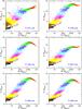 |
Fig. 9 Temporal evolution of the planetary M − R diagram after the final masses have been reached. The colors show the fraction of heavy elements Z = MZ/M in a planet. Orange: Z ≤ 1%. Red: 1 < Z ≤ 5%. Green: 5 < Z ≤ 20%. Blue: 20 < Z ≤ 40%. Cyan: 40 < Z ≤ 60%. Magenta: 60 < Z ≤ 80%. Yellow: 80 < Z ≤ 95%. Brown: 95 < Z ≤ 99%. Black: Z > 99%. |
7.3.1. Evolution at early times
At an age of 10 Myr (top left-hand panel), some planets still have very large radii. The M − R relationship is at this moment still considerably different from the shape at later times. For massive giant planets, we see that there is a significant spread in associated radii for one mass. This is a visible imprint of different formation histories, namely, of the initial entropy of these planets. The initial entropy for giant planets depends on the way the gas and the solids have been accreted during the formation phase. High gas accretion rates in the runway phase, for example, make the “cold start” scenario more similar to the “hot start” scenario (see Spiegel & Burrows 2012). This is because at a high gas accretion rate, a planet accretes a lot of matter when its radius is still relatively big. As a result, the accretion shock is weak, leading to a relatively high entropy of the accreted gas. This in turn leads to a large radius. The entropy of young planets will be studied in a dedicated work on the planetary luminosities (Mordasini et al., in prep.).
At an age of 50 Myr, we start to recognize the characteristic shape of the planetary M − R relation. It first consists of small radii for low-mass planets, followed by an increase of the radius with mass up to a local maximum of the radius at about 4 Jovian masses and finally a decrease of the radius with mass in the super-Jupiter domain. The latter is a consequence of the well-known fact that the degree of degeneracy in the interior increases (e.g., Chabrier et al. 2009), which gives the planetary M − R relationship an overall shape reminiscent of an elongated “S”.
We currently do not include deuterium burning. This means that the radii of objects more massive than 13 MX at times when D burning occurs (t ≲ 0.1 − 1 Gyr) will be too small.
7.3.2. Evolution at late times
The relative shape of the M − R relation hardly changes between an age of 500 Myr and 5 Gyr. The planets slowly contract on Gyr timescales and thus move vertically downwards, keeping their relative position. The vertical movement can be seen by looking, e.g., at the local radius maximum in the giant planet domain.
At these late times, the spread in radius at a given mass no longer comes directly from their different accretion histories, but instead from their different heavy element contents. The fact that, for a given mass, a planet with a higher heavy element content has a smaller radius gives rise to the diagonal pattern seen in the color coding, as illustrated by the following example for t = 5 Gyr. When we move at a fixed radius of, say, 7 R⊕ from left to right across the envelope of points, we first encounter planets with a mass of about 20 M⊕ and a heavy element content of 40% to 60% (cyan). However, when we move further right to higher masses, Z must increase in order to keep the same radius of 7 R⊕. Therefore, at a mass of about 100 M⊕, the color changes from cyan to magenta, indicating that the planets now have a heavy element fraction of 60% to 80%. In other words, when we fix the heavy element content and increase the mass, the radius also increases, leading to diagonal bands of identical color. Obviously, this is only true in the domain where the radius is an increasing function of mass (M ≲ 4 MX).
In addition, the distance from the star plays a certain role for the radius, with objects closer to the star having a larger radius (e.g., Fortney et al. 2007). As the minimal allowed radius is 0.1 AU, the effect is, at least for giant planets, not so large, and of order 0.5 to 1 R⊕. This is different for the few close-in, low-mass (M < 10 M⊕), gas-rich (up to 20% gas) planets that are visible close to the left-hand border of the plot. As expected, such planets have (Fig. 3; Rogers et al. 2011) large radii (up to 5 or 10 R⊕, depending on age) that increase with decreasing mass. The radius of these planets is affected by the simple gray atmosphere model, as discussed in Sect. 2.2.2. It is also clear that such objects are sensitive to envelope evaporation, especially just after formation, when they have very large radii, sometimes exceeding 15 R⊕. The effects of envelope loss will be included in future work.
The calculation of the radius for a given age, composition, and orbital distance can be done in a purely evolutionary model, too. But only a combined formation and evolution model in a population synthesis calculation gives a prediction for both the spread of the radii for a given mass domain and the distribution of the radii. When looking at the vertical width in radius that the envelope of points covers, we see that, depending on mass, there are regimes where all planets have nearly the same radius (very massive giant planets). In other mass domains, there is a very significant spread in possible radii. In Sect. 7.9, we show histograms of the radius distribution for different mass domains. For example, at t = 5 Gyr and a mass of about 40 M⊕, we find planets with radii between about 3 and 9 R⊕, i.e., a variation of a factor three. The reason is that in this mass domain both clearly solid-dominated planets (95 < Z ≤ 99%) and small gaseous planets (20 < Z ≤ 40%) exist. Not all types are, however, found at all semimajor axes (see Sect. 7.7).
7.3.3. General shape of the M – R relation
Concerning the overall shape of the planetary M − R relation, we see that low-mass planets have small radii because they consist mostly of solids, while high-mass planets have large radii because they consist mostly of gas. This is clearly visible from the color coding showing the decrease of the heavy element fraction Z = MZ/M with mass. This decrease is a direct consequence of the fact that during formation low-mass cores cannot accrete large amounts of gas because their Kelvin-Helmholtz timescale is too long. Such planets never undergo gas runaway accretion. Massive, super-critical cores must always accrete significant amounts of gas symmetrically (at least if they form during the lifetime of the gaseous disk) as they necessarily must trigger runaway gas accretion. Neither a (nearly) core-free, e.g., 10 M⊕ planet (which would have a radius of ~1 RX at 1 AU, Fortney et al. 2007), nor a pure 3 MX ice planet (which would have a radius R ~ 0.4 RX, Sect. 2.1.1) can form in the core accretion scenario. Combined with the fundamental properties of matter as expressed in the EOSs, this leads to the two “forbidden” regions in the planetary M − R plane in the top left and bottom right, resulting in a shape of the M − R relationship similar to an elongated “S”. We see that the synthetic M − R relationship contains the imprint of the basic concepts of the core accretion formation theory.
7.4. Comparison with the observed M – R relation
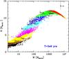 |
Fig. 10 Comparison of the synthetic and the observed M − R relationship. The synthetic population and all actual planets with known mass and radius (both in the solar system and around other stars) and a semimajor axis of at least 0.1 AU are shown. For extrasolar planets, error bars are given. The color code for the internal composition of the synthetic planets is the same as in Fig. 9. The synthetic population only contains planets with primordial H2/He atmospheres, thus at low masses discoveries of planets lying below the synthetic population are expected. The two “forbidden” regions in the top left and bottom right are a consequence of the core accretion formation process (and the EOS). This leads to a characteristic, elongated “S” shape of the planetary M − R relationship. |
Figure 10 shows again the synthetic population at 5 Gyr, but now together with all actual planets that have a semimajor axis larger than 0.1 AU (as in the model) as well as a well-constrained mass and radius. We additionally plot Kepler-20d (Gautier et al. 2012) and Kepler-10c (Fressin et al. 2011), for which only upper mass limits are known, as unfortunately is the case for many other interesting Kepler planets, like those around Kepler-30 or Kepler-11g (Fabrycky et al. 2012; Lissauer et al. 2011a). The observational data was taken from exoplanets.org (Wright et al. 2011) on 23.3.2012. The host stars of the planets are roughly solar-like, with masses between about 0.7 and 1.3 M⊙. In the synthesis, the stellar mass is fixed to 1 M⊙. For simplicity, we also include the circumbinary planets Kepler-34b, Kepler-35b, and Kepler-16b (Welsh et al. 2012; Doyle et al. 2011).
It is clear that the age of the observed planets is not exactly 5 Gyr, so the comparison can only be approximate. For a more exact comparison, each planet should be compared individually with the synthetic population at its specific age. A comparison of the general structure of the M − R diagram can, however, still be made for two reasons. First, all host stars shown here are thought to be old main-sequence stars, causing typical uncertainties in the age of an individual star of several gigayears and often allowing for an actual age of 5 Gyr. Second, the evolution of the radius at such a late time is very slow. The radius of a 1 MX planet decreases, for example, between an age of 1 and 5 Gyr only by about 0.4 R⊕ (Paper I).
Looking at the envelope of the actual and synthetic planets, we note that the observed planets all lie in the envelope covered by the synthetic population if we take into account the error bars, with the clear exception of KOI-423b (Bouchy et al. 2011). Except for this planet, there is thus a good agreement between the model and the observation.
For planets with a mass similar to Jupiter or higher, we see that the observed planets seem to be distributed over the entire vertical width of the envelope of the synthetic planets. For planets with a mass similar to Saturn or less, one notes that the observed planets cluster at the upper boundary of the envelope covered by the synthetic planets. As discussed in Sect. 7.7 below, an explanation for this could be an imprint of the semimajor axis. Synthetic planets at all semimajor axes are shown here (i.e., between 0.1 AU and ~20 AU), while the observed exoplanets are close to the lower limit of this range. For planets at even lower masses (Neptunian mass domain), observed planets of a similar mass can have very different radii. This is illustrated by Kepler-18d (Cochran et al. 2011), which has a mass similar to Neptune, but is about 1.8 times as large in radius. Clearly, this reflects that the spread in possible heavy element contents is large. We assume that the atmospheric composition is always solar. It is clear that different chemical compositions would lead to different opacities, which in turn lead to different cooling histories and radii (cf. Burrows et al. 2011, for the brown dwarf regime). This would further increase the vertical width of the envelope.
7.4.1. Individual objects
The internal composition of the actual extrasolar and solar system planets shown in Fig. 10 has been analyzed in numerous works with more detailed physics than used here. It is therefore important to understand to what extent the results of these studies can be reproduced with our simpler model.
In Table 3, we list the inferred fraction of heavy elements Z in the individual planets shown in Fig. 10, assuming again an age of 5 Gyr. To derive these fractions, only the position in the M − R plane was used. Additional constraints like the semimajor axis or the metallicity of the host star were not considered here. The third column of the table shows the composition of the synthetic planet that lies closest to the observed values in the M − R plane. A ~symbol means that either no reasonably close synthetic planet was found in the M − R plane or that for the planet, observationally, only upper limits of the mass are known. The fourth column shows possible Z found in the rectangle in the M − R plane covered by the error bars of the observations. Values for solar system objects are assumed to be exact.
Derived fraction of heavy elements Z = MZ/M in planets with a > 0.1 AU.
The general trend that the heavy element fraction Z = MZ/M decreases with increasing mass is obvious. It is worth looking at some extrasolar planets individually. Starting at the smallest masses (≲10 M⊕), we see that the low-mass planets around Kepler-10 (Fressin et al. 2011), Kepler-11 (Lissauer et al. 2011a), and Kepler-20 (Gautier et al. 2012) can be reproduced with envelopes masses of ~1 to ~20% of the total mass of the planets, similar to what was found by Lissauer et al. (2011a).
It is expected that at such low masses and a ≥ 0.1 AU, planets will be found in future with radii smaller than in the synthetic population. Such objects have already been found at very small orbital distances, for example, Kepler-10b with M = 4.6 M⊕, R = 1.4 R⊕ and a semimajor axis of 0.017 AU (Batalha et al. 2011). This is much closer than the domain we currently model in our simulations. Objects with an Earth-like composition without H2/He are, however, also expected to exist at larger semimajor axes, as demonstrated by the terrestrial planets in the solar system. From the comparison of such objects with the domain covered in the synthesis, it will become possible to constrain the transition from terrestrial and water planets to mini-Neptunes (with primordial H2/He envelopes). This helps to understand various processes of primordial envelope accretion and loss, which is difficult from the solar system alone with its large gap in mass between the Earth and the ice giants.
Kepler-18d (Cochran et al. 2011) is a remarkable planet with a mass (16.4 ± 1.4 M⊕) approximately between that of Neptune and Uranus, but a radius that is 80% larger than Neptune. It thus seems to have a clearly lower heavy element fraction than the two solar system planets. As can be seen in Fig. 10, this planet lies in the M − R diagram at the upper border of the M − R region covered with synthetic planets. We derive a heavy element fraction of 0.43 to 0.52 (MZ = 7.1 to 8.5 M⊕), similar to Cochran et al. (2011), who find a MZ = 10.4 ± 1.4 M⊕. Such a composition of about half gas and half solids does not exist in the solar system. As described in Mordasini et al. (2012c), we find that planets of such a composition can only form if the grain opacity in the envelope during the formation phase is much smaller than the interstellar grain opacity. This object is thus important to constrain uncertain parameters of the core accretion model. A complication arises from the fact that at a semimajor axis of about 0.12 AU, this planet might still get affected by the irradiation of the host star in a more complex way than modeled here. Then it could have a relative composition closer to the solar system ice giants.
The system of the two Saturn-mass planets Kepler-9b and Kepler-9c (Holman et al. 2010) has been analyzed in detail in Havel et al. (2011). Comparing our simpler analysis with their more sophisticated calculations still indicates a relatively good agreement: Havel et al. (2011) derive for Kepler-9b and an age of 5 Gyr (as in our calculation) a possible range of Z between 0.19 and 0.56, with a nominal value of 0.37. For Kepler-9c, also at 5 Gyr, they derive a Z between 0.17 to 0.58, with a nominal value of 0.37. Our simulations indicate a heavy element fraction for Kepler-9b of 0.24 to 0.30 with a nominal value of 0.25, while for Kepler-9c values of 0.16 to 0.36 with a nominal value of 0.30 are found. The allowed ranges thus agree in the two analyses. The smaller nominal values in our analysis are not surprising, as the effect of additional heating in the envelope of the planet due to stellar irradiation is not taken into account in our simulations. Therefore, lower core masses are sufficient to explain the observed radius. In Havel et al. (2011), the effect of irradiation leads to an uncertainty of about 30% for the value of Z. The error bars in their analysis are larger (and more realistic) because more sources of uncertainties like atmospheric opacities are taken into account.
For Jupiter, we find that the closest synthetic planet contains about 31 M⊕ of heavy elements, similar to what we describe in Paper I. This is in good agreement with the allowed range for the total amount of heavy elements found by Guillot (1999) of 11 to 41 M⊕. For Saturn, the derived heavy element mass is 25.6 M⊕, also in good agreement with Guillot (1999) who finds masses between 19 and 31 M⊕. For the ice giants, we find that they contain about 10 to 12% of gas, similar to what was found by, e.g., Hubbard et al. (1991).
CoRoT-10b (Bonomo et al. 2010) has a mass of about 880 ± 51 M⊕ and is interesting because it seems to contain a high fraction of heavy elements despite its high mass, as already noted in Bonomo et al. (2010). These authors infer that 120 to 240 M⊕ of heavy elements should be contained in the planet. We find that this planet should contain about 150 M⊕ of metals, assuming that the star is 5 Gyr old, which is compatible with their result. In the M − R plane, the planet lies towards the lower boundary of the domain covered with synthetic planets, but still well within it. Planets with such high solid masses can also form by core accretion without collision in metal-rich disks (high [Fe/H] and high gas mass) at large semimajor axes of ~10 AU. An example of the formation of such a planet is shown in Mordasini et al. (2009a). Compared to the formation of Jupiter, the isolation mass is much larger under such circumstances, allowing for the accretion of many more planetesimals so that the plateau phase II (Pollack et al. 1996) is skipped. It should, however, be noted that such a formation is probably only feasible if the random velocities of the planetesimals remain low while the planet grows (“monarchical” growth, Weidenschilling 2005).
The most massive object in the comparison, KOI-423b (Bouchy et al. 2011) with a mass of approximately 5800 M⊕ ( ≈ 18 MX), cannot be explained with our model, which assumes standard cooling sequences with solar composition opacities. The same conclusion was reached by Bouchy et al. (2011). These authors show that large ad hoc increases in the atmospheric opacities are necessary to reconcile the measured mass and radius with cooling models, given the high age of the host star (estimated to be between 3.6 and 6.6 Gyr). With the assumptions of our model (solar opacities, no bloating mechanisms), we can only reproduce the large radius if we assume an age of the planet of less than 100 to 500 Myr. This object is currently difficult to understand from a theoretical point of view, as stated already by Bouchy et al. (2011).
In summary, we see that our simple model leads to estimated heavy element contents that agree relatively well with the results from more detailed models. However, an important factor for this agreement is unfortunately that despite great efforts, the latter studies can also deduce the internal composition, including that of the solar system planets, only with significant error bars. This is due, e.g., to the uncertainties in the equations of state, the distribution of heavy elements (mixed vs. layered structure), the efficiency of convection, and the currently limited amount of observational data. The reader is referred to Fortney & Nettelmann (2010) or Baraffe et al. (2010) for recent reviews.
7.4.2. Constraints from a multi-dimensional parameter space
Due to the still limited number of extrasolar planets with an accurately known mass and radius at large orbital distances, the analysis shown here represents only the very beginning of the possible constraints that can be derived in future from the planetary M − R relationship.
Once large numbers of planets with accurately measured mass, radius, semimajor axis, host star mass, and metallicity are known, it will be possible to compare observation and theory with Kolmogorov-Smirnov tests and to search for correlations in this multi-dimensional parameter space. An already known example is the correlation between stellar [Fe/H] and planetary heavy element content (Guillot et al. 2006; Burrows et al. 2007; Miller & Fortney 2011). This correlation can be reproduced with planet population synthesis calculations (Mordasini et al. 2009b; 2011b).
In Sect. 7.7, we will show a correlation between semimajor axis and radius found among synthetic planets. It is particularly important to have many well-characterized planets with semimajor axes clearly larger than 0.1 AU. This should reduce the impact of several poorly understood mechanisms influencing close-in planets during their formation (e.g., the exact disk structure close to the inner rim) and evolution (strong irradiation), thus making it possible to see the correlations more clearly.
7.5. Bimodal planetary radius distribution
A prediction of the planetary radius distribution is one of the most important results of a population synthesis calculation and is similar in its importance as a prediction of the planetary mass function (Ida & Lin 2008; Mordasini et al. 2009b). Figure 11 shows the distribution of the radii of all synthetic planets with a radius larger than 2 R⊕ at an age of 5 Gyr. Planets at all semimajor axes are included. The distribution is normalized, i.e., the sum of the fractions in all bins is unity. Table 4 lists the corresponding fractions at ages of 1, 5 and 10 Gyr.
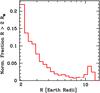 |
Fig. 11 Predicted radius distribution for planets with primordial H2/He atmospheres and a radius R > 2 R⊕. Synthetic planets at all semimajor axes have been included. The age of the population is 5 Gyr. |
Radius distribution for planets with a primordial H2/He atmosphere and R > 2 R⊕.
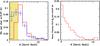 |
Fig. 12 Left panel: number of planets per star in a given radius bin and an orbital period P < 50 d (a < 0.27 AU for a 1 M⊙ star). The thick red line is the synthetic population. The blue line with error bars is from Howard et al. (2012) for the Kepler data of Feb. 2011 (Borucki et al. 2011). The black dotted line is the preliminary analysis of Howard et al. (2011) for the data of Sep. 2011 (Batalha et al. 2012). The observational data in the hatched region with R < 2 R⊕ is incomplete. Right panel: normalized fraction of radii of the same synthetic planets as on the left, but with finer bins, and including only planets with R > 2 R⊕. |
The distribution has a characteristic, bimodal shape (cf. Schlaufman et al. 2010; Wuchterl 2011): a global maximum at the smallest radii and a second, lower local maximum at a radius of about 1 RX. The increase towards small radii is due to the increase of the underlying mass distribution towards small masses, combined with the fact that with decreasing mass, the fraction of heavy elements increases (Sect. 7.3). This means that low-mass planets also have small radii. It is well possible that the increase towards small radii may be even stronger in reality than predicted by the model. This is due to the fact that we only include (relatively large) primordial H2/He envelopes and one embryo per disk.
There is also a fundamental reason for the second maximum at about a Jovian radius: In the giant planet domain (M ≳ 100 M⊕), planets all have approximately the same radius, independent of their mass. This is in turn due to the property of matter to become degenerate for such massive objects (e.g., Chabrier et al. 2009). This property of the EOS causes a high number of planets from a wide range of different masses to all fall into the same radius bin (radii between ~0.9 and 1.1 RX), resulting in the maximum in the distribution. The local minimum of the distribution occurs at a radius of 7 to 8 R⊕. As can be deduced from Fig. 10, this corresponds to masses between ~20 to ~200 M⊕, with a typical mass of ~70 M⊕. This coincides roughly to the mass domain of the “planetary desert”, where several planet formation models based on the core accretion theory (e.g., Ida & Lin 2008; Mordasini et al. 2009b) predict a lower abundance of planets. This additional effect makes the second maximum even more prominent.
The figure shows the radius distribution at the specific age of 5 Gyr. In reality, stars of a given observational sample will have a distribution of ages. The evolution of the radii at late times (t ≳ 1 Gyr) is, however, slow. The distribution of the radii in an age range between 1 to 10 Gyr changes only slightly. As expected, there is still a slow general contraction, so that at an age of 1 Gyr instead of 5 Gyr, for instance the local maximum in the giant planet domain is shifted by one bin to the right (i.e., by about 0.1 RX). But the general shape remains very similar, as can also be seen from Table 4.
Our results become increasingly uncertain with decreasing radius. This is due to the fact that we do not model several effects that are important for planets with small radii, such as the concurrent formation of many planets in one disk and the loss of the gaseous envelope due to evaporation. This and the fact that we only include primordial H2/He envelopes, whereas in reality there are also planets with other types of atmospheres (or without atmosphere), means that the actual radius distribution could be substantially different from the synthetic one for smaller radii. The comparison of the synthetic and the actual distribution then helps to quantify these effects.
7.6. Comparison with Kepler results
It is interesting to compare the radius distribution found in the synthesis with the one observed by the Kepler satellite (Borucki et al. 2011). Howard et al. (2012) have analyzed the radius distribution of Kepler planet candidates with high signal-to-noise transits for a subsample of bright GK dwarfs. They corrected for the observational bias to derive the underlying radius distribution for planets with R > 2 R⊕ and an orbital period of less than 50 days. In Fig. 12, we compare their observational result with the synthetic radius distribution.
In the left-hand panel we show, as do Howard et al. (2012), the number of planets per star in a given radius bin and a semimajor axis <0.27 AU. Synthetic planets that migrate to the inner border of the computational disk at 0.1 AU are evolved at this orbital distance. The majority of planets analyzed by Howard et al. (2012) are found outside of 0.1 AU, as the planetary frequency increases with distance, especially for companions that are not giant planets. This means that the comparison of our synthetic planets with 0.1 ≤ a/AU ≤ 0.27 with the sample of Howard et al. (2012), which includes all planets inside ~0.27 AU, can still be made, at least in an approximate way.
7.6.1. Agreement for R ≳ 2 R⊕
The number of planets per star can be directly calculated from the synthesis because the outcome for all simulated planets is known3. We see that the synthetic and the observed result are in good agreement, especially for the new preliminary analysis of Howard et al. (2011) for the updated Kepler data set released in Sep. 2011 (Batalha et al. 2012). Both data sets are characterized by an increase of the frequency with decreasing radius. The slope of the increase is similar in both cases, with the synthesis predicting a somewhat higher number of planets with a small radius. In addition to the relative increase, the absolute number of planets is similar in the model and observation. This could indicate that the inward migration of planets (especially at low masses, i.e., in type I) is quite efficient. The total fraction of stars with a planet with P < 50 d and R > 2 R⊕ in the synthesis is 20.1%. The value derived from Kepler is 16.5% to 20% (Howard et al. 2012; 2011).
However, the very good agreement (also in absolute terms) must be regarded with caution, particularly because we are using the one-embryo-per-disk approximation. As a result, we cannot take into account that the occurrence rate calculated by Howard et al. (2012) includes multiple-planet systems and gives the number of planets per star, which can be higher than one, while it is exactly one in our simulations by construction when considering all synthetic planets. Including only one planet per star would reduce the number of Kepler candidates by about 20% (Latham et al. 2011; Wolfgang & Laughlin 2012) and mainly lead to a reduction of planets with small radii. Planets with small radii are more frequently found in multiple systems, while giant planets are more often single (Latham et al. 2011). But the basic result remains: both the model and the synthesis find a strong increase towards small radii, and this increase follows a similar slope.
7.6.2. Divergence for R ≲ 2 R⊕
Figure 12 shows that the synthetic radius distribution decreases for radii smaller than ~2 R⊕. The reason for this is that low-mass planets with a H2/He atmosphere, even when it is only tenuous (0.1 to 1% of the core mass), have radii of at least ~2 R⊕ at the relevant equilibrium temperatures for a < 0.27 AU and ages (i.e., intrinsic luminosities) (see Fig. 3). This is in agreement with the findings of Rogers et al. (2011). As we only model this type of atmosphere and even low-mass cores accrete such amounts of gas during the formation phase, there are not many synthetic planets with a radius smaller than ~2 R⊕. It is clear that our quantitative results for the distribution of the radii of very low-mass planets are strongly affected by the various simplifications in the model, for example, the assumption of chemically homogeneous layers (in particular of a pure H2/He envelope) or the fact that we neglect the evaporation of the envelope. On the other hand, the basic mechanism responsible for the decrease of the radius distribution, which is the M − R relationship of close-in, low-mass planets with H2/He atmosphere, should not be affected by this. We checked that the decrease remains similar if we start the simulations with embryos with a mass of 0.1 instead of 0.6 M⊕.
This decrease is in contrast to the (however incomplete) observational result (Howard et al. 2012) where the fraction remains at least constant for R < 2 R⊕ (see also Youdin 2011). The good agreement of the synthetic and the actual radius distribution for R > 2 R⊕ as well as the divergence at smaller radii are interesting. It could indicate that for planets larger than ~2 R⊕, H2/He atmospheres are dominant (mini-Neptune type of planets), while for smaller radii, other types of planets (silicate-metal terrestrial planets or ocean planets without primordial H2/He) dominate. While our quantitative results are as mentioned to be taken with great caution, this result seems to be in agreement with detailed analyses of the combined constraints coming from the Kepler data for the radius and from RV for the mass (Howard et al. 2012; Wolfgang & Laughlin 2012; Gaidos et al. 2012). These studies show that with decreasing radius, a transition from low planetary densities to higher densities occurs. In particular, Wolfgang & Laughlin (2012) find that when they use a mixture of planets with H2/He atmospheres and rocky planets, the latter type of planets becomes dominant for radii R ≲ 2.5 R⊕ for their simulation that best reproduces the combined constraints from HARPS and Kepler. This is similar to the result found here from theoretical calculations. The results on the radius distribution of planets with primordial atmospheres presented here and in Sect. 7.8 should allow for an even better understanding of the dividing line between these types of planets.
7.6.3. Local maximum at ~1 RX
The left-hand panel of Fig. 12 shows the synthetic planets in the same bins as the observed data. No peak in the giant planet regime can be seen due to the broadness of the bins. The right-hand panel shows the same synthetic planets, but now using finer bins (and R > 2 R⊕). The bimodal shape of the radius distribution becomes visible again. The local maximum at about 1 Jovian radius is, however, about two to three times smaller than for the distribution that includes synthetic planets at all semimajor axes (Fig. 11). This is due to the fact that giant planets are less frequent inside 0.27 AU than further out.
At the resolution of the radius distribution in the current observational data and the restriction that P < 50 d, it is thus difficult to see the bimodality. If we use finer bins (which is possible with a higher number of transiting planets), or if we keep the same broader bins, but include planets at all semimajor axes, the peak at about 1 Jovian radius should become visible. This is an important prediction, which is in agreement with other models of planet formation and evolution (Schlaufman et al. 2010; Wuchterl 2011). It will be tested in the next few years with the Kepler mission as an increasing number of planets at large semimajor axes will be found. We must distinguish two aspects of the local maximum at about 1 RX: the local minimum at a radius of about 8 R⊕ and the sharp absence of planets larger than ~1.2 RX. The second aspect is more fundamental, as it is a direct consequence of the EOS. When making the comparison, we must keep in mind a number of possible complications that could cause differences between the synthetic and the actual radius distribution.
1) First of all, it is clear that the results shown here can only be compared with planets that are not affected by the various proposed inflation mechanisms (e.g., Batygin et al. 2011). An inflation to larger radii naturally blurs the maximum at one specific radius, as found in standard cooling calculations conducted here. It is interesting to note that Demory & Seager (2011) find that at irradiation fluxes of less than about 2 × 10⁸ erg cm-2 s-1 giant planets seem not to be significantly affected any more by inflation. For a solar-like star, the critical irradiation level corresponds to a semimajor axis of about 0.07 AU. Instead, all giant planets in their sample are characterized by a constant radius of ~0.87 ± 0.12 RX. This is compatible with our results for the location of the local maximum in the radius distribution.
2) It is possible to construct a mass distribution that has no maximum at about 1 Jovian radius. First, such a mass distribution must contain a higher number of planets with intermediate radii compared to the synthetic mass distribution, so that the local minimum at about 8 R⊕ disappears. This would mean that the “planetary desert” (Ida & Lin 2004; dedicated discussion in Mordasini et al. 2009a) is more populated than found in the model. In this case, the radius distribution between ~6 and 12 R⊕ would simply be flat or decrease with R. Second, the mass distribution could contain a lower number of giant planets. This would naturally lower the number of planets in the second maximum. When comparing the fraction of planets with radii close to 1 RX in the model and in the data of the Kepler satellite (left-hand panel of Fig. 12), one notes that the number of synthetic giant planets is in good agreement with the observed fraction. This would mean that this second possibility is in fact not feasible.
3) Demory & Seager (2011) find that the majority of Kepler candidates of their sample, which receive only a modest irradiation flux but still have large radii ≳1.1 RX, have to be classified as “ambiguous” candidates, i.e., as cases where the secondary eclipse signature is consistent with both a planetary and stellar companion and not as relatively clear planetary companions, as is the case for most candidates with smaller radii. This could indicate that some of the Kepler candidates that are difficult to understand from a theoretical point of view (radius clearly larger than 15 to 20 R⊕, orbital period longer than 10 to 20 days, high age) are false positives. False positives would also blur the upper radius limit of planets. A finding of Traub (2012) could also point in this direction: he finds that in the Kepler data there are significantly more candidates around faint stars than around brighter host stars for large planets with radii of about 8 to 40 R⊕. This is not to be expected for astrophysical reasons, so Traub (2012) puts forward the explanation that it is more difficult to distinguish background eclipsing binaries from planetary transits when the stars are faint. This would mean that this radius class is more affected by false positives. As more data are accumulated by Kepler, it should become possible to better assess such a reason. It is also interesting that when Kepler candidates in multiple systems only are considered (Latham et al. 2011), the observed radius distribution is bimodal. A minimum at about 1 RX and a local maximum at about 1.2 RX are seen, which is at least qualitatively similar to what we found in our simulations here. The number of planets in the relevant bins is however very small, so that it is currently unclear whether this is a statistically significant result.
4) The synthetic radius distribution shows planets that all have exactly the same age. While in the Kepler data the majority of the host stars are on or close to the main sequence (Batalha et al. 2012; Latham et al. 2011), the spread in ages will blur to some extent the maximum at about 1 RX, especially its upper edge, which is in contrast very sharp in the synthetic population at one single age. A similar effect is expected from our simplification that all planets have identical atmospheric opacities.
5) Finally, objects like KOI-423b (Bouchy et al. 2011), which are quite far from theoretical expectations, could indicate that our theoretical understanding of the planetary radius evolution does not take into account all relevant mechanisms that affect at least some planets. Possible mechanisms could be, for example, tidal heating for very eccentric planets (Dong et al. 2012) or giant impacts (Anic et al. 2007).
7.7. Impact of the semimajor axis
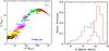 |
Fig. 13 Left panel: synthetic M − R relationship as in Fig. 10, but including only synthetic planets with a final semimajor axis smaller than 1 AU. The color coding and the observational comparison sample is the same as in Fig. 10. Right panel: distribution of radii of planets with masses between 100 and 300 M⊕. The red solid line is for planets with a semimajor axis less than 1 AU, while the black dashed-dotted line shows planets outside of this distance. Planets reaching the inner border of the computational disk have been excluded. The age of the population is 5 Gyr. |
Figure 10 shows the M − R relationship for synthetic planets at all semimajor axes, including planets at large orbital distances. Observationally, most of the known transiting planets have in contrast small semimajor axes. To see the impact of the semimajor axis on the radii, we plot agin in Fig. 13, left-hand panel, the M − R relationship, but now including only synthetic planets with a semimajor axis between 0.1 and 1 AU. The extrasolar planets in the observational comparison sample all have semimajor axes less than 1.1 AU (the planets of the solar system are found at larger distances, of course).
7.7.1. Semimajor axis – radius anticorrelation
Comparing the synthetic planets at smaller distances with the entire population shows that there is a clear difference. At all masses, the lower part of the envelope of M − R points corresponding to those planets with the smallest radii for a given mass are not found if only the planets inside 1 AU are considered. This reduces the vertical width of the area populated by M − R combinations, so that Kepler-10c and CoRot-10b now lie at the lower boundary of the region populated by synthetic planets. When all semimajor axes are included, they are more embedded in the cloud of points. This is because the maximum mass fraction of heavy elements Z for a given total mass is lower for planets inside 1 AU than for those further out. For example, planets with a total mass of 100 M⊕ can contain up to ~90% solids (in rare cases, though) when considering all semimajor axes (Fig. 10). When limiting to a ≤ 1 AU, the heavy element fraction is at most ~60%, as can be seen in Fig. 13.
This is a consequence of the following. The reservoir of solids available for a planet to accrete in a disk with a dust-to-gas ratio fD/G scales with distance r as fD/GΣ(r,t = 0)r2, where Σ(r,t = 0) is the initial surface density of gas. This quantity is given by Eq. (A.1), and thus scales in the inner, relevant parts of the disk as r-0.9. This means that the amount of mass contained in an annulus increases with semimajor axis. This trend gets amplified by the increase of the solid surface density at the iceline. It is clear that this radial dependence gets blurred by orbital migration, but as the simulations show, the general pattern remains conserved.
It is interesting to see that the actual known extrasolar planets of the comparison sample (which have semimajor axes between 0.1 and 1.1 AU) mostly cluster close to the upper edge of the synthetic population, at least for intermediate masses between ~50 to 300 M⊕, and thus seem more similar to the synthetic population inside 1 AU than to synthetic planets further out. No planet with a mass of, e.g., 100 M⊕ and a radius of only 6 R⊕ has been detected to date, despite such metal-rich objects existing in the synthetic population at large distances (Fig. 10). The right-hand panel of Fig. 13 compares the distribution of radii for a similar mass domain for planets in- or outside 1 AU. The difference is very obvious. The better match of the observed planets with the synthetic population inside 1 AU could indicate that also in nature close-in giant planets contain a smaller fraction of heavy elements than their counterparts further out, which formed in a larger reservoir of solids. Kepler-18d has a mass similar to the ice giants in the solar system, but is much poorer in solids (Sect. 7.4.1). This could point in the same direction.
This makes it possible to make the following two statements. First, for the ongoing high-precision transit searches, it is predicted that they will find intermediate and giant planets with a higher fraction of heavy elements (i.e., smaller radius) as they detect planets at larger semimajor axes. Second, this anti-correlation of semimajor axis and radius via Z might offer a possibility to distinguish between disk migration and other mechanisms, like scattering (Malmberg et al. 2011) or Kozai migration (Fabrycky & Tremaine 2007), as formation mechanisms of close-in hot Jupiters. This is because it is at least not obvious that the latter two mechanisms would also lead to a semimajor axis – Z correlation as found here for disk migration.
7.7.2. Possible complications
A number of complications arise. First, it seems reasonable to assume that a higher bulk content in metals goes along with a higher atmospheric opacity. Higher opacities are well-known to delay the contraction of giant planets (e.g., Burrows et al. 2011; Paper I). In this work, in contrast, we use opacities for solar composition gas in all cases. The impact of higher opacities for more metal-rich planets would counteract the semimajor axis-radius anti-correlation. Second, the evolution of the radius of a giant planet is also influenced directly by its semimajor axis via the intensity of the stellar irradiation. When the irradiation flux is not deposited deep in the interior of the planet, this does not have a very drastic influence on the radius for a > 0.1 AU. For instance, a Jovian mass planet at 0.1 AU has at 4.5 Gyr a radius that is about 6% larger than a counterpart at 10 AU (Fortney et al. 2007). At least for planets inside 0.1 AU, there are however special inflation mechanisms that affect the radius much stronger, as illustrated by the large number of transiting planets with anomalously large “bloated” radii. It is currently not clear out to which distance these inflation mechanisms are effective deepening on, e.g., the planetary mass or composition. The inflation also leads to an anti-correlation of semimajor axis and radius, i.e., goes in the same direction as the correlation describe here due to the composition, thus complicating the picture.
In summary, we see that the combined constraints of planet mass, radius, semimajor axis and metallicity provide powerful observational constraints for planet formation and evolution theory, in particular when they are coupled to population synthesis calculations that make it possible to see the correlations between these quantities. However, a step to be taken in future for more accurate analyses is a more self-consistent coupling of bulk interior composition and atmospheric properties in terms of composition and opacity.
7.8. Mean radius as function of mass
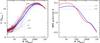 |
Fig. 14 Left panel: synthetic M − R
relationship with analytical approximations for the mean
radius |
Several studies (e.g., Howard et al. 2012;
Wolfgang & Laughlin 2012; Gaidos et al.
2012) have analyzed combined radial RV and
Kepler data sets because they enable insight into the mean density of
the planets. An important quantity in this context is the power-law
exponent β, which relates planetary mass and radius
 (23)It is clear that
in reality, there cannot be a single value of β (and k)
for all planetary masses and compositions. Still, it remains a useful quantity when
comparing theory and observations.
(23)It is clear that
in reality, there cannot be a single value of β (and k)
for all planetary masses and compositions. Still, it remains a useful quantity when
comparing theory and observations.
Observationally, a fit to the terrestrial planets of the solar system yields β = 0.33, like for constant density spheres (Laughlin & Wolfgang 2012), while a fit including the Earth and Saturn (Lissauer et al. 2011b) gives β = 0.48, with k = 1 in both cases. From theoretical calculations, one expects for scaled versions of the Earth in the 1 − 10 M⊕ regime β ≈ 0.27 (Valencia et al. 2006) and β ≈ − 1/8 for massive gaseous planets of about 10 MX (Chabrier et al. 2009), as expected from polytropic models. The negative values show that in this domain the radius decreases with mass. At the maximum of the M − R relationship at about 4 MX (Fig. 10), β must be equal to zero. This means that with increasing mass, a decrease of β occurs. This is a consequence of the combined effects of a change in the interior composition of the planets with mass (the gas fraction increases) and increasing degeneracy of the matter. The specific dependence of β on mass is a proxy for the bulk interior composition of the planets.
7.8.1. Analytical expression for the mean radius
To calculate β, we first have to find an analytical expression for the
mean radius as function of mass  for which the best-fitting parameters for the synthetic population are determined. We
employ the function proposed by Traub (2011),
which has four
parameters b,M0,w,p and
is given as
for which the best-fitting parameters for the synthetic population are determined. We
employ the function proposed by Traub (2011),
which has four
parameters b,M0,w,p and
is given as  (24)where log denotes the
logarithm to the base 10. The units in the fit are Earth masses and radii. Compared to
the original function of Traub (2011), we have
omitted an additional additive constant that is found to be unnecessary. In the
equation, the parameter p controls how abruptly the radius increases
when going from terrestrial planets to the maximum in the giant planet regime. It also
controls how flat the maximum in the giant planet regime is. The
parameter w controls the width of the peak in the radius function.
The parameter M0 is the mass (in units of Earth masses)
corresponding to the maximum radius (i.e., four to five Jovian masses),
while b provides a vertical scaling. The value of b
corresponds to the radius (in units of Earth radii)
at M = M0.
(24)where log denotes the
logarithm to the base 10. The units in the fit are Earth masses and radii. Compared to
the original function of Traub (2011), we have
omitted an additional additive constant that is found to be unnecessary. In the
equation, the parameter p controls how abruptly the radius increases
when going from terrestrial planets to the maximum in the giant planet regime. It also
controls how flat the maximum in the giant planet regime is. The
parameter w controls the width of the peak in the radius function.
The parameter M0 is the mass (in units of Earth masses)
corresponding to the maximum radius (i.e., four to five Jovian masses),
while b provides a vertical scaling. The value of b
corresponds to the radius (in units of Earth radii)
at M = M0.
We have fitted our nominal population at 5 Gyr with this function using a nonlinear least-squares Marquardt-Levenberg algorithm to find the parameters. We only include planets with a mass larger than 2 M⊕. The result is shown in Table 5 and Fig. 14. The best-fitting parameters are given for all planets that have not reached the inner border of the computational disk (i.e., 0.1 < a/AU) and for a selected semimajor axis range 0.1 < a/AU ≤ 1 to study again the effect of the semimajor axis. Planets that reach the inner border of the computational disk are excluded from the analysis since their fate is more uncertain.
Fitting parameters for the  relationship.
The left-hand panel of Fig. 14 shows that the fit (thick lines) yields a good representation of the mean synthetic M − R relationship. In the plot, the thin colored lines show the mean radius found directly with a running mean with a window 0.15 dex wide in log (M/M⊕). The fitting function and the running mean lie in general close to each other, except for a few special fine features that the fitting function cannot reproduce. As expected from the discussion in the last section, the line including only planets inside 1 AU lies at larger radii for intermediate mass planets. With the two sets of parameters, one finds a radius of about 1.8 and 1.6 R⊕ for a 1 M⊕ planet. Clearly, this is a consequence of only simulating planets with primordial H2/He atmospheres.
7.8.2. Mass-radius power-law exponent
The power-law exponent β is given as
 .
The power-law exponent for Traub’s (2011) fit is
given as (ln is the natural logarithm)
.
The power-law exponent for Traub’s (2011) fit is
given as (ln is the natural logarithm)  (25)Three different regimes
can be distinguished for β. The mean planetary density decreases with
increasing mass for β > 1/3
and is independent of mass for β = 1/3, while values
of β smaller than 1/3 indicate that the density is increasing with
mass. The right-hand panel of Fig. 14 shows the
value of β as a function of mass, again for the two different semimajor
axis ranges. The exact numerical values of β partially depend on the
specific fitting function. Using, for instance, polynomial functions instead of
Eq. (24) leads to variations
of β by of order 0.05 to 0.1, but preserves the general pattern.
At small masses, the values of β are relatively large.
For M ≲ 30 M⊕ and when all planets
with a > 0.1 AU are included (blue line),
then β lies between 0.3 and 0.33, close to the constant density case.
This is the result of two counteracting effects: the increase of the gas-mass fraction
in the planets with increasing mass tends to lower β, while the growing
effect of gravitational self-compression of the more compressible gas tends to
increase β. When only planets inside 1 AU are included (red line),
then β is higher (0.35 to 0.4), showing that for these planets, the
density decreases with increasing mass, due to the smaller heavy element content
(Sect. 7.7). At a mass of roughly
100 M⊕, β starts to decrease as the
effect of self-gravitational compression takes over, reaching β = 0 at
a few Jovian masses, as expected.
(25)Three different regimes
can be distinguished for β. The mean planetary density decreases with
increasing mass for β > 1/3
and is independent of mass for β = 1/3, while values
of β smaller than 1/3 indicate that the density is increasing with
mass. The right-hand panel of Fig. 14 shows the
value of β as a function of mass, again for the two different semimajor
axis ranges. The exact numerical values of β partially depend on the
specific fitting function. Using, for instance, polynomial functions instead of
Eq. (24) leads to variations
of β by of order 0.05 to 0.1, but preserves the general pattern.
At small masses, the values of β are relatively large.
For M ≲ 30 M⊕ and when all planets
with a > 0.1 AU are included (blue line),
then β lies between 0.3 and 0.33, close to the constant density case.
This is the result of two counteracting effects: the increase of the gas-mass fraction
in the planets with increasing mass tends to lower β, while the growing
effect of gravitational self-compression of the more compressible gas tends to
increase β. When only planets inside 1 AU are included (red line),
then β is higher (0.35 to 0.4), showing that for these planets, the
density decreases with increasing mass, due to the smaller heavy element content
(Sect. 7.7). At a mass of roughly
100 M⊕, β starts to decrease as the
effect of self-gravitational compression takes over, reaching β = 0 at
a few Jovian masses, as expected.
Towards the lowest masses (2 M⊕), β decreases slightly with decreasing mass. This is because at sufficient irradiation from the host star the radius of low-mass planets with a significant H2/He atmosphere increases with decreasing total mass when the heavy element fraction Z is held constant (see Fig. 3). This would correspond to negative values of β. The effect that for the synthetic planets Z is itself increasing with decreasing mass, however, overcompensates this. Due to this imprint of formation (lower mass cores can only bind smaller envelopes during the formation phase), very low values of β do not occur at low planetary masses, especially as we have excluded planets with a ≤ 0.1 AU. The fact that the power-law exponent for low-mass planets with H2/He atmospheres is found to be similar to that of solid planets without atmospheres could make the observational distinction more difficult. In terms of absolute sizes, the two planetary types are however clearly distinct.
We stress that the fit is not expected to provide a good representation of the planetary M − R relationship at low masses in the terrestrial and super-Earth regime. The terrestrial planets of the solar system and some low-mass extrasolar planets like CoRot-7b or Kepler-10b do not possess primordial H2/He envelopes. But the comparison of the predicted and the actual M − R relationship allows insight into the actual nature of such objects, in particular when studying the fraction of silicate-iron or water planets versus mini-Neptunes (Wolfgang & Laughlin 2012; Gaidos et al. 2012).
7.9. Radius distribution for given mass intervals
In the previous section, the mean radius as function of mass was studied. The mean radius can however not catch that for every mass planets with different internal compositions, and thus different radii, form in the synthesis. The importance of such a multi-valued M − R relationship for the interpretation of Kepler and RV data has been stressed by Wolfgang & Laughlin (2012). These authors also consider terrestrial planets without any atmosphere, while we only consider planets with primordial H2/He atmospheres. But already for this single type of planet, there is a large diversity in M − R relations. We therefore plot in Fig. 15 the distribution of the radii for nine mass intervals, ranging from super-Earth planets to objects in the brown dwarf regime. In each panel, the radii of planets with semimajor axes of 0.1 < a/AU ≤ 3 are included. Planets reaching the feeding limit are not included here, as their evolution is most affected by mechanisms that we do not model (e.g., evaporation). The outer border is chosen so that the distributions do not become too dominated by planets at even larger distances, facilitating comparison with observational data.
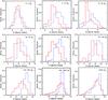 |
Fig. 15 Distribution of radii of planets with primordial H2/He envelopes for nine mass domains as indicated in the plot. Synthetic planets with 0.1 < a ≤ 3 AU are included. The red solid line is the nominal population, while the blue dashed-dotted line is a population where isothermal type I migration rates reduced by a factor 10 were used. In the panels showing the lowest mass domains, the fine gray lines show the distribution of the core radii. The age of the population is 5 Gyr. |
In each panel, the distribution for the nominal population is shown. Additionally, we plot the radius distribution of another, non-nominal population. This population was calculated in an identical way as the nominal one, except that instead of the new type I migration model (Sect. 7.1.1), we use the migration rates derived by Tanaka et al. (2002) for a locally isothermal disk, reduced by a global efficiency factor fI = 0.1. The comparison of the results for the two populations makes it possible to quantify the impact of an aspect of the planet formation model that is still not very well understood.
In the first two panels showing the lowest mass intervals, we also plot the core radius distribution. One sees that the total radii are typically much larger than the core radii, despite the fact that these planets are dominated by solids, as can be seen in Fig. 10. The effect that an H2/He envelope of, e.g., 1% in mass around a super-Earth planet strongly increases the radius is well known (e.g., Rogers et al. 2011; Fig. 3). We comment that the low grain opacity that is assumed during the formation phase (fopa = 0.003, see Mordasini et al. 2012c) is responsible for low-mass cores of, e.g., 5 M⊕ accreting envelopes with masses up to ~15% of the total mass during the lifetime of the protoplanetary disk.
Table 6 lists the numerical values of the mean, standard deviation and skewness of the radius distribution of the different mass bins. A positive (negative) skewness indicates that an asymmetric tail is extending to larger (smaller) radii, while a distribution, which is approximately Gaussian, has a vanishing skewness.
Statistical properties of the radius distribution (in Earth radii) of planets with a primordial H2/He envelope at an age of 5 Gyr.
The histogram and the table show that the mean is increasing with mass except for the
highest mass range, as expected. Note that the mean values listed here only agree in an
approximative way with the mean radius  found with Eq. (24). This is because the
two values were derived with a different ansatz (fit over the entire population versus
mean in a given mass domain) and the semimajor axis domains of the planets included in the
analyses are different. The table shows that the standard deviations can be significant,
as is also the total spread of the radii.
found with Eq. (24). This is because the
two values were derived with a different ansatz (fit over the entire population versus
mean in a given mass domain) and the semimajor axis domains of the planets included in the
analyses are different. The table shows that the standard deviations can be significant,
as is also the total spread of the radii.
Regarding the skewness, one sees that a clear pattern only develops for the largest masses. In the mass bin going from 300 to 1000 M⊕, the clearly negative skewness is due to the general shape of the planetary M − R relationship (see Fig. 10) and the fact that some planets in this mass regime contain so many solids that this has a non-negligible effect on the total radius. For the largest mass bin (M > 3000 M⊕), the negative skewness is in contrast caused by the decrease of R with M at such masses.
7.9.1. Impact of the migration model
While the distributions of the two populations are to first order similar, we note that in almost all panels the distribution of the non-nominal population (isothermal type I migration) is shifted towards larger radii. This means that the planets in the non-nominal population have in general a smaller heavy element fraction Z, which can be understood from the different migration models: the new type I migration model allows for both in- and outward migration. In some cases, this means that the net inward migration is smaller, saving in this way planets from getting close to the star. This does, however, not mean that the total annulus in the disk visited by the planet is small, as the absolute migration rates are also high in the non-isothermal regimes, at least as long as a planet does not get captured into a convergence zone (cf. Lyra et al. 2010; Mordasini et al. 2011a). Since we follow Pollack et al. (1996) in assuming low planetesimal random velocities, the total mass of heavy elements that a planet can accrete is proportional to the annulus of the disk swept by it. This annulus is larger for the non-isothermal migration at full strength than for the isothermal migration reduced arbitrarily by a factor ten. This leads to the difference in the heavy element fraction. Only for the planets more massive than 3000 M⊕ does the difference in the heavy element content between the two populations have nearly no visible consequences any more for the total radius. These planets are too strongly dominated by gas.
When comparing the distributions found here with observations, one should keep in mind that the lower the mass range, the larger the uncertainties. Planets with a mass less than ~10 M⊕ will be affected in the strongest way by the limitation that we do not model any growth process once the protoplanetary disk is gone. We only consider primordial atmospheres, neglect evaporation, and compositional changes due to outgassing as well as non-solar opacities.
7.10. Core and total radius
In Sect. 2.1, we studied the radius of the solid cores of the planets as a function of mass, composition, and external pressure. Figure 16 shows the mass-core radius relationship in addition to the normal M − R diagram. Lines indicate the theoretical M − R for planets without a gaseous envelope.
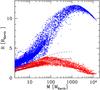 |
Fig. 16 Total and core radius as a function of mass for all planets with M > 2 M⊕ at 5 Gyr. The total radius is shown by blue diagonal crosses, while the core radius is shown by red open squares. The dashed line is the M − R relation for solid planets with an icy composition (approximative solar composition beyond the iceline with 75% ice, 17% silicates and 8% iron). The solid line is for solid planets with an Earth-like rocky composition (2:1 silicate-to-iron ratio). These two lines show the radius if no external pressure is acting. |
Concerning the core radius of low-mass planets, we see that at low total masses (M ≲ 10 M⊕) the core radii cluster close to two groups, which are found at (or slightly below) the dashed and solid lines which indicating a purely icy and rocky composition, respectively. This is expected, as the composition of the two classes of solids is the same in all simulations and corresponds to a solar-like composition (see Sect. 2.1.1). In reality, due to the fact that stars do not have simply a scaled solar composition (e.g., Delgado Mena et al. 2010), there will be a spread both in the composition of refractory and volatile material in the planets (Bond et al. 2010). Giant impacts can additionally modify the iron and water fraction (e.g., Marcus et al. 2009). At these masses (M ≲ 10 M⊕), there are however also some cores that lie between the solid and the dashed line. These are planets that have migrated from outside the iceline into the inner part of the disk, so that they have a mixed composition. The frequency of such close-in “ocean” planets is an important and possibly observable diagnostics of the efficiency of migration. Some core radii lie slightly below the two lines. This comes from the fact that for such cases the pressure exerted by the gaseous envelope is already sufficient to compress the core by a small degree.
When comparing total and core radii of low-mass planets, we see that there are some cases with a total radius that lies between the solid and the dashed line. These are planets that are made of a rocky core and tenuous amounts of gas, resulting in a radius smaller than that of an atmosphere-free icy planet. This is a manifestation of the well-known degeneracy of the M − R relation for low-mass planets. The combination of mass and radius measurements with spectroscopy (e.g., with the Exoplanet Characterization Observatory (EChO) mission, Tinetti et al. 2011) is therefore very important for a better understanding of this part of the planetary M − R relationship.
At masses between 10 to 100 M⊕, the effect of the compression of the core due to a massive envelope becomes clearly visible, so that the points indicating the actual core radii diverge from the lines indicating radii of planets without significant envelopes. At very high masses (M ≳ 10 MX), cores get very strongly compressed to sizes that are smaller than the core radii of the low-mass planets (Rcore ≲ 1 R⊕). Clearly, it is questionable whether a solid core can survive for 5 Gyr at the extreme conditions found in the center of such planets without being eroded, as we currently assume for simplicity. Recent results on the solubility of ice in conditions as found in Jupiter’s center (Wilson & Militzer 2012) indicate that at least for this planet, core erosion is possible. It is therefore of interest to take such effects into account. On the other hand, it is also clear that the higher the total mass, the smaller the relative fraction it contains in solids as indicated by the color coding in Fig. 10. This plot shows that planets with masses higher than ~10 MX have a core mass fraction Z of 5% to less than 1%, decreasing with total mass. This means that the total radius is only slightly influenced by the core mass, as reflected in the vertical width of the M − R relationship in Fig. 10, which becomes very narrow at such large masses. This finding could partially be changed if we included different opacities (e.g., Burrows et al. 2011).
8. Summary
In the first part of this paper, we have described several improvements and extensions of our combined formation and evolution model.
8.1. Planet module
First, we included the calculation of the radius of the solid core as a function of its mass, composition, and (for giant planet cores) external pressure by solving the internal structure equations for a differentiated planet. We compared our results with previously published studies (e.g., Seager et al. 2007) and found very good agreement (Sect. 2.1.1). We can therefore make relatively accurate predictions for the radii of core-dominated planets, necessary for comparison with high-precision transit missions like Kepler. We further found that the variable core density only has a small impact on the formation phase of a giant planet, but that it needs to be considered for correct total radii of (giant) planets at late times. These radii are essential to estimate the heavy element content of a giant planet (Sect. 5).
Second, we have developed a simple model for the core luminosity due to the decay of long-lived radionuclides. We assumed a chondritic composition of the mantel and took into account the temporal decay of the nuclides (Sect. 2.3). For a low-mass, close-in super-Earth planet with a ~1% primordial H2/He atmosphere we demonstrated that the radioactive decay becomes the dominant intrinsic heat source at late times. This leaves traces in the temporal evolution of the radius of the planet. We compared our results with Rogers et al. (2011) and found good agreement (Sect. 6). This means that we can address in population synthesis calculations the radii of low-mass planets with tenuous primordial envelopes. This is an important subject because low-density, low-mass planets are currently being detected in large numbers (Borucki et al. 2011) and because these detections are linked to the habitability of low-mass planets.
8.2. Disk module
We have presented improvements of the protoplanetary gas disk module, which is a 1+1D α model including the effects of stellar irradiation and photoevaporation. We now use more realistic initial conditions (Andrews et al. 2009), a free outer radius of the disk that allows spreading and shrinking, and an updated photoevaporation model that takes into account external and internal photoevaporation (Sect. 3.1). With this model, we studied the stability against self-gravity and found that disks with masses up to 0.091 or 0.16 M⊙ (without and with stellar irradiation, respectively) are stable for the characteristic radius and initial surface density slope we assume. We also found that the radius of the lowest Toomre parameter in these disks occurs around 25 AU, close to the location we determined analytically (Appendix A).
8.3. Planetary mass-radius relationship
In the second part of the paper, we have used the updated model to conduct planetary population synthesis calculations. In contrast to earlier syntheses, we can now not only calculate the planetary semimajor axis-mass diagram, but also the M − R diagram. Also, the mass-luminosity and semimajor axis-luminosity diagrams are now a self-consistent result of the model that will be presented in future work. The planetary M − R diagram is of similar importance as the semimajor axis-mass diagram because it enables a first characterization of a planet via its bulk composition.
We have presented how the planetary M − R relationship for planets with primordial H2/He envelopes (the only type of atmosphere we currently model) comes into existence during the formation phase (when planets grow) and how it then evolves over gigayear timescales during the evolutionary phase at constant mass. During the presence of the nebula (Sect. 7.2), two regimes exist for the radii: low-mass, subcritical cores have very large radii comparable to the Hill sphere (or Bondi) radius because their envelopes are attached to the background nebula, whereas supercritical cores have massive, collapsed envelopes with radii of a few RX. Most planets, however, do not trigger runaway gas accretion, but instead undergo a phase of rapid contraction when the nebula disappears.
During the evolutionary phase (Sect. 7.3) for t ≳ 0.5 Gyr, the basic shape of the M − R relationship is similar to an elongated “S”, which can be understood from the fundamental principles of the core accretion model, and the EOS. Due to their long Kelvin-Helmholtz timescale, low-mass planets cannot bind massive gas envelopes, whereas super-critical cores necessarily must trigger runway gas accretion (at least if they form during the lifetime of the protoplanetary disk). This naturally leads to two “forbidden” regions in the M − R plane: one at low masses with large radii and one at high masses with small radii (Sect. 7.3.3).
The radius of a planet for a given composition and age can also be calculated in purely evolutionary calculations. The spread in possible associated radii for a given mass interval (i.e., the vertical width of the M − R relationship) and the distribution of the radii in a specific mass range can, however, only be obtained from combined formation and evolution calculations. We find that, depending on the mass domain, there is a large diversity in the associated radii. At a mass of ~40 M⊕ for example, radii vary by a factor ~3. This is mainly due to different bulk compositions, reflecting different formation histories. We present the synthetic radius distribution for various mass intervals in Sect. 7.9.
When comparing the synthetic M − R relationship with the observed one (Sect. 7.4), one finds good agreement with the planets of the solar system and for actual exoplanets with a > 0.1 AU, which corresponds to the minimal orbital distance of the synthetic planets. All exoplanets with a ≥ 0.1 AU and the planets of the solar system fall in the M − R envelope populated with synthetic planets (Fig. 10), except for one case (KOI-423b). We derive approximate heavy elements contents for the individual observed planets (Sect. 7.4.1). The general trend is that the fraction of iron, silicates and ices decreases with increasing mass, but there is significant spread for individual objects.
We then show the synthetic planetary radius distribution at 5 Gyr, which is a fundamental result of population synthesis calculations (Sect. 7.5). The radius distribution is bimodal and characterized by a strong increase towards small radii and by a second, lower local maximum at a radius of about 1 RX. The increase towards small radii is a consequence of the increase of the planetary mass function towards low M and the fact that low-mass planets cannot accrete much nebular gas. This means that low-mass planets also have small radii. The second local maximum at about 1 RXis due to a fundamental property of matter (degeneracy) causing the radius to be nearly independent of mass in the giant planet domain. Due to this, planets from a wide mass range all fall in the same radius bin, leading to the local maximum at about 1 RX.
A comparison of the synthetic radius distribution with the observations of the Kepler satellite (Howard et al. 2012) shows a good agreement for R ≳ 2 R⊕, but a divergence for smaller radii (Fig. 12). While our quantitative results for low radii are to be taken with great caution, this could indicate that for R ≳ 2 R⊕ the radius distribution can be relatively well described with planets with primordial H2/He atmospheres (as in the model), while at smaller radii, planets of a different nature dominate. This result seems to be in good agreement with analyses combining data from Kepler and RV surveys (Wolfgang & Laughlin 2012; Gaidos et al. 2012). We predict that in the next few years, Kepler should find the second, local maximum at about 1 RX. We also predict that the typical radii of planets with 10 ≲ M/M⊕ ≲ 1000 will decrease with distance. This stems from a positive correlation of the semimajor axis and the typical fraction of heavy elements in a planet. The reason for this is that the amount of solids in an annulus increases for our disk surface density profile (Sect. 7.7).
To facilitate comparison with observations, we used the analytical expression of Traub (2011) to derive the mean radius as function of mass in the synthetic population (Sect. 7.8) and studied the M − R power-law index β (M ∝ Rβ). The value of β is between 0.3 to 0.4 for planets with M ≲ 100 M⊕. At higher masses, β decreases to reach zero at about 4 MX, and negative values at even higher masses. As we only considered primordial H2/He atmospheres, it is expected that at low masses the observed M − R relation will diverge from the synthetic result.
9. Conclusion
With the extensions and improvements presented in Paper I and this study, we are now able to characterize extrasolar planets in their most important physical quantities, like semimajor axis, mass, composition, radius, and luminosity from one single model. These quantities are calculated in a self-consistent way for the coupled formation and evolution of a planet during its entire life, from a tiny seed embryo in the protoplanetary disk to a gigayear-old planet. Our goal is to have in the end synthetic populations that can be compared directly with all important observational techniques used to find and characterize exoplanets. We believe that a better theoretical understanding of the very complex patterns in the various data sets (like transiting planets of very different compositions, systems of compact close-in low-mass planets, cold Neptunes beyond the iceline or massive, directly imaged giant planets at large distances) can best be developed by comparing theoretical results to a combination of all these data sets. In the current case, the combined results of transit and RV measurements make it possible to conclude that first, for a > 0.1 AU, the actual and the synthetic M − R relationships are in good agreement, and second, that for radii larger than roughly 2 R⊕, the synthetic radius distribution is similar to the one detected by Kepler. Finally, we find that the planetary radius distribution is bimodal, with the global maximum at low radii and a second smaller maximum at about 1 RX. We predict that Kepler will detect this maximum in the next few years.
Online material
Appendix A: Stability of irradiated α disks against self-gravity
In population synthesis calculations (e.g., Ida & Lin 2004; Mordasini et al. 2009a), one uses distributions of (initial) protoplanetary disk masses in order to reflect the varying initial conditions for planet formation.
As discussed in Sect. 3.2, massive cold disks get self-gravitationally unstable, which would invalidate the usage of a classical α model with one constant α across the disk. Ida & Lin (2004) and Mordasini et al. (2009a) have therefore cut off the uppermost part of the observed disk mass distribution with the argument that they cannot be stable. The cut off was usually done at the (often assumed) disk mass stability limit of about a tenth of the stellar mass, without a direct calculation of this stability limit. Observationally, high disk masses can be mimicked by residual dust in the remains of the envelope from which the star formed, contributing to the observed flux (Andrews & Williams 2005).
In this Appendix, we use our upgraded disk model to determine the maximum stable disk mass for both irradiated and non-irradiated disk and make some more general remarks about the stability of irradiated α disks against the development of spiral waves and clumping.
For simplicity, we use for the initial disk profile (Eq. (7)) a power-law exponent γ = 0.9 and a
characteristic radius Rc = 30 AU. Both values correspond to
the maxima of the distributions observed by Andrews et al. (2010). With these values, the initial gas surface density is
![Mathematical equation: \appendix \setcounter{section}{1} \begin{equation} \Sigma(r,t=0)=\Sigma_0\left(\frac{r}{5.2\, \mathrm{AU}}\right)^{-0.9}\exp\left[-\left(\frac{r}{30\, \mathrm{AU}}\right)^{1.1}\right]\cdot \label{eq:newprofile} \end{equation}](/articles/aa/full_html/2012/11/aa18464-11/aa18464-11-eq354.png) (A.1)It is clear
that this procedure faces difficulty because it implicitly assumes that we can use the
observed dust grains to trace the mass and evolution of the gas. Especially grain growth
could make this assumption partially invalid (e.g., Andrews & Williams 2007).
(A.1)It is clear
that this procedure faces difficulty because it implicitly assumes that we can use the
observed dust grains to trace the mass and evolution of the gas. Especially grain growth
could make this assumption partially invalid (e.g., Andrews & Williams 2007).
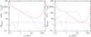 |
Fig. A.1 Toomre parameter QToomre (red solid line) and τcoolΩ (blue dotted line) as a function of semimajor axis a at a moment shortly after the beginning of disk evolution. The horizontal lines correspond to the critical values of QToomre,crit = 1.7 and τcoolΩ = 3, respectively. The left panel is for a disk with an initial mass Md(t = 0) = 0.024 M⊙, while the right one corresponds to a higher mass, Md(t = 0) = 0.11 M⊙. |
When integrating Eq. (7) from
r = 0 to infinity using the parameters mentioned before, one finds a
total initial disk mass (cf. Miguel et al. 2011) of 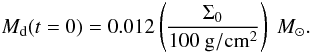 (A.2)Thus, the MMSN of
Weidenschilling (1977, 2005) corresponds to Σ0 ≈ 200 g/cm2, while for
Hayashi’s (1981) MMSN of
0.013 M⊙, Σ0 ≈ 108 g/cm2. It is
likely that the true initial mass of the solar nebula was a few times larger than these
minimal masses (Weidenschilling 2005).
(A.2)Thus, the MMSN of
Weidenschilling (1977, 2005) corresponds to Σ0 ≈ 200 g/cm2, while for
Hayashi’s (1981) MMSN of
0.013 M⊙, Σ0 ≈ 108 g/cm2. It is
likely that the true initial mass of the solar nebula was a few times larger than these
minimal masses (Weidenschilling 2005).
We note that we do not allow in the model accretion rates larger than 3 × 10⁻⁷ M⊙/yr in order to avoid convection in the vertical direction, but if necessary reduce locally the initial Σ in order not to exceed this limit. Therefore, the initial gas mass for disks with Σ0 larger than ~1000 g/cm2 is somewhat smaller than predicted by Eq. (A.2). For Σ0 = 2000 g/cm2, the initial mass is, for example, about 20% smaller than given by Eq. (A.2). We note further that in contrast to earlier models, we can now include the total disk mass inside the computational domain and not only the fraction contained in the innermost 30 AU (Mordasini et al. 2009a).
A.1. QToomre and τcoolΩ as function of distance
Figure A.1 shows QToomre (solid red lines) and τcoolΩ (blue dotted lines) as a function of distance from the star for two disks (see also Bell et al. 1997) at t ≈ 0 (the moment we start the disk evolution). The left-hand panel shows a 1 − 2 × MMSN disk (Md(t = 0) = 0.024 M⊙, Σ0 = 200 g/cm2), while the right one shows a more massive disk with Md(t = 0) = 0.11 M⊙ (Σ0 = 1000 g/cm2). Both examples are calculated including the effect of stellar irradiation on the disk temperature structure, M∗ = 1 M⊙, α = 7 × 10⁻³ and the initial surface density profile discussed above.
We see that for both disks, QToomre reaches a minimum at about 25 AU. For the MMSN disk, the minimum value is about 12, while for the more massive disk, it is 2.5. The critical value of QToomre,crit ≈ 1.7 is not reached. Regarding the cooling, the particular structure of the curve is due to opacity transitions. We see that in the inner parts of the disk and outside 15 − 25 AU, there are parts of the disk that could in principle cool quickly enough, so that τcoolΩ < 3. The cooling timescale is the time in which the disk would cool if we suddenly switched off the heating mechanisms. This is however meaningless for gravitational fragmentation due to the too high values of Q everywhere in the disks. Therefore, fragmentation does not occur, either.
We have studied the overall minimal QToomre,min occurring in disks as a function of time, radius, and Σ0 in order to determine the maximum Σ0 that can be used. In these calculations, we again assume α = 7 × 10⁻³ and M∗ = 1 M⊙. It is found that the minimal QToomre always occur very shortly after the start of the disk evolution (within some 104 years) and that afterwards QToomre always increase. Thus, the minimal QToomre are a direct consequence of the initial conditions (as expected), and the disks evolve towards stability.
A.2. Radius of maximum instability
The orbital distance where the overall minimal
QToomre,min occur correspond to
about 20 AU for disks calculated without stellar irradiation and, as also seen in the
two examples in Fig. A.1, to about 25 AU for
disks with irradiation, independent of the disk mass and as long as
Md(t = 0) ≲ 0.1 − 0.2 M⊙.
For more massive disks, the distance of the minimal Q increases. This
result can be understood at least for the irradiated disks if we assume that in the
outer parts the temperature structure is given by the stellar irradiation only. We can
consider two cases: first, an optically thin disk with
Tmid ∝ r − 1/2.
In this case, the orbital
distance RToomre,min,t
where the minimal QToomre,min occurs is
given for γ < 7/4 as
(using Eqs. (7), (10) and
Tmid ∝ r − 1/2)
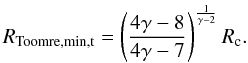 (A.3)This corresponds
to ratios
RToomre,min,t/Rc = 1/4,
3/4, 0.791, 0.886 for a disk surface density exponent (Eq. (7))
γ = 3/2, 1, 0.9, and 1/2.
(A.3)This corresponds
to ratios
RToomre,min,t/Rc = 1/4,
3/4, 0.791, 0.886 for a disk surface density exponent (Eq. (7))
γ = 3/2, 1, 0.9, and 1/2.
Second, we can consider a passively irradiated disk without viscous dissipation,
where for orbital distances between about 0.4 and 84 AU,
Tmid ∝ r − 3/7
(Chiang & Goldreich 1997). In this
case, one finds an orbital
distance RToomre,min,p
where the minimal QToomre,min occurs at
 (A.4)This corresponds
to ratios
RToomre,min,p/Rc = 0.18,
0.71, 0.76, 0.87 for γ = 3/2, 1, 0.9, and 1/2. We
see that the results for an optically thin and a passively irradiated disk are
similar. This is due to the fact that the temperature depends in both cases in a
similar way on the distance.
(A.4)This corresponds
to ratios
RToomre,min,p/Rc = 0.18,
0.71, 0.76, 0.87 for γ = 3/2, 1, 0.9, and 1/2. We
see that the results for an optically thin and a passively irradiated disk are
similar. This is due to the fact that the temperature depends in both cases in a
similar way on the distance.
For Rc = 30 AU and γ = 0.9, this leads for a passively irradiated disk (which is the situation assumed here, see Fouchet et al. 2012) to a RToomre,min,p = 22.8 AU, close to the result ( ≈ 25 AU) seen in the simulations. The somewhat larger value in the simulations is likely due to residual viscous heating.
In Fig. A.2 we plot the overall
minimum QToomre,min (i.e., the lowest
value reached at any distance and time) as a function of Σ0
(or equivalently the initial disk mass), for disks with (red solid) and without (blue
dotted) irradiation. In both cases, Q follows a simple power-law that
scales as  ,
as expected from Eq. (10).
,
as expected from Eq. (10).
One sees that Q is higher in disks with irradiation, which is expected as these disks are hotter and thus more stable, in particular in the outer regions, where Q becomes small and where viscous heating is not important.
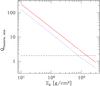 |
Fig. A.2 Overall minimal Toomre parameter QToomre,min as a function of initial gas surface density at 5.2 AU, Σ0 which is a direct proxy of the initial disk mass (Eq. (A.2)). The red solid line is for disks with irradiation, the dotted blue one is for disks where viscosity is the only heating source. The dashed line gives the critical value of 1.7. |
From Fig. A.2 we find a maximum initial gas surface density Σ0,max (measured at 5.2 AU) leading to stable disks (QToomre,crit = 1.7) for disks without irradiation of 790 g/cm2, corresponding to an initial disk mass of 0.091 M⊙, while for disks with irradiation, the maximum allowed value is 1510 g/cm2, corresponding to an initial mass of 0.16 M⊙.
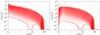 |
Fig. B.1 Gas surface density Σ in a protoplanetary disk as a function of distance and time. The surface density is plotted in intervals of 2 × 10⁴ years. The uppermost line shows a state shortly after the beginning of disk evolution. The lowermost line is the profile when the calculation is stopped. The two panels differ from each other by the boundary condition that is used at the inner edge of the disk at 0.1 AU, as described in the text. All other parameters are identical and given as M∗ = 1 M⊙, α = 7 × 10⁻³ and Σ0 = 200 g/cm2. |
A.3. Global instability
At disk masses higher than ~10 − 25% the mass of the central object, the possibility of global gravitational instability must be considered, too (e.g., Harsono et al. 2011).
The particular case of global instability to m = 1 modes (one-armed spirals) has been studied numerically and analytically in Adams et al. (1989) and Shu et al. (1990). If this mode is amplified by the SLING mechanism (which is due to the fact that for a one-armed spiral, the star is displaced through the conservation of the center of mass), there is a finite threshold for the instability to set in, which is a function of the Toomre criterion. For the case that QToomre = 1 at the outer disk edge, it is possible to derive analytically a critical disk mass, below which the disk is gravitationally stable against all modes. In a linear stability analysis, Shu et al. (1990) find for this situation a critical “maximum-mass solar nebula” at Mdisk/(Mdisk + M∗) = 3/(4π), corresponding to Mdisk/M∗ = 0.31.
The analytical analysis of Shu et al. (1990) suffers from a number of limitations (cf. Noh et al. 1992 for a discussion), and might not be applicable in the strict sense in the context here. There are two reasons for this: Our disks have a smooth outer edge, so that they might not reflect the density waves, and in addition, for our disks, the minimal Q does not occur at the outer disk edge, but further in (Eq. (A.4)). If we compare the critical disk mass of Shu et al. (1990), Mdisk/M∗ = 0.31, we find, despite the limitations with the most massive disk stable to local disturbances for the model here (Mdisk/M∗ = 0.16), we find that the disks should also be globally stable.
Since the works of Adams et al. (1989) and Shu et al. (1990), many studies have revisited the question of (global) disk stability. While a direct connection to the SLING mechanism can in general not be made (Nelson et al. 1998), it is nevertheless found that at constant Q, with increasing Mdisk/M∗, the character of the instability changes. At low Mdisk, thin, multi-armed structures develop that are characterized by high-order patterns (m ≳ 5), whereas at high Mdisk, global, low order (m = 2 − 5) instabilities dominate (Nelson et al. 1998). The transition between the two regimes occurs at approximately Mdisk/M∗ = 0.2 − 0.4. These results are confirmed at much higher numerical resolution by Harsono et al. (2011) and Lodato & Rice (2004). The latter authors find that local effects dominate as long as the disk mass is less than 0.25 M∗ and the disk aspect ratio H/R ≲ 0.1. Our massive disks are characterized by H/R between 0.06 to 0.09 in their outer parts, so that they fulfill this criterion.
These results indicate that the transition from local to global instabilities might rather be a gradual one and not set in at a specific disk mass, as originally advocated by Shu et al. (1990). The disk mass where global effects become important seems to be at about 0.25 M∗ (Nelson et al. 1998; Lodato & Rice 2004; Harsono et al. 2011), which is comparable to the original criterion by Shu et al. (1990). These results indicate that our most massive, Toomre-stable disk with 0.16 M⊙ should also be stable to global modes. We must, however, keep in mind that the numerical simulations mentioned here did not use exactly the same surface density and temperature profile. Therefore, in order to get a firm conclusion, dedicated hydrodynamic simulations are necessary.
Appendix B: Characteristic disk evolution under the influence of photoevaporation
In this Appendix, we illustrate the characteristic evolution of the protoplanetary disks under the combined action of viscosity and photoevaporation, as found in the update model, in order to check our results against previous studies. Figure B.1 shows the gas surface density as a function of time for a disk with α = 7 × 10⁻³, Σ0 = 200 g/cm2, and a mean external photoevaporation rate over the lifetime of the disk of about 7 × 10⁻⁹ M⊙/yr. The effects of irradiation on the thermal structure of the disk is taken into account as described in Fouchet et al. (2012). These initial conditions result in a disk lifetime of 2.0 Myr (remaining disk mass 10-5 M⊙). In the figure, a line is plotted all 2 × 10⁴ years, and the minimal allowed surface density is set to 10-3 g/cm2.
The two panels of the figure differ only by the inner boundary condition at Rmin = 0.1 AU. In the left-hand panel, we use the same boundary conditions as in our earlier models, which means that the flux through the innermost cell instantaneously adopts to the flux coming from further out. This is equivalent to the statement that the disk structure would continue to some smaller radius inside 0.1 AU, which is not modeled. In the right-hand panel, Σ is forced to fall to zero at 0.1 AU. Physically, we can associate the two situations with different sizes of the magnetospheric cavity, i.e., with a weak and a strong magnetic field of the host star, respectively (e.g., Bouvier et al. 2007). A detailed description of the structure of the disk close to the host star that takes into account magnetic fields will be presented in an upcoming work (Cabral et al., in prep.).
While the inner boundary condition has a very strong impact on the migration behavior of low-mass planets close to the star (Benitez-Llambay et al. 2011), it has otherwise no effect on the characteristic evolution of the disk.
B.1. Phases during disk evolution
Figure B.1 shows that the evolution of the disk can approximatively be separated in four phases:
-
1.
The initial exterior radius specified by the initial conditions getsquickly reduced by external photoevaporation to a radius wheremass removal due to photoevaporation, and the viscousspreading of the disk are in a quasi-equilibrium, as described byAdams et al. (2004). In the specific case, the radiusdecreases from initially about 200 AU to ~100 AU. In the inner part, the disk very quickly evolves from the initial profile towards equilibrium.
-
2.
In the second, dominant phase a quasi self-similar evolution of the disk occurs. The inner part of the disk (r ≲ 10 AU) is in near equilibrium (i.e., the mass accretion rate is nearly constant as a function of radius), and the slope of the gas surface density γ is approximately −0.9 (but varying between −0.4 and −1.5 due to opacity transitions). The outer radius is slowly moving inwards, from about 100 AU to 60 AU. For more massive disk, this equilibrium radius is further out.
-
3.
Once the surface density has fallen to about 0.01−0.1 g/cm2 at ~10 AU, a gap opens somewhat outside of Rg,II. The evolution of the disk now speeds up, which corresponds to the so-called “two-timescale” behavior (Clarke et al. 2001).
-
4.
Quickly afterwards, the total disk mass has fallen to 10-5 M⊙, where we stop the calculation. We note that the evolution at very small Σ is not important for our purpose of planet-formation modeling. Therefore, we currently do not include the effect of the direct radiation field, which would clear the disk quickly from inside out once the gap has opened (Alexander & Armitage 2009).
Such an evolution is very similar to the findings of previous studies (Matsuyama et al. 2003; Clarke et al. 2001). We note that the evolution can become more complex if there is additionally a planet accreting significant amounts of gas. This is the case if the planetary core becomes massive enough to trigger gas runaway accretion, so that a giant planet forms. Such a planet then effectively acts as a sink cell in the disk (see Paper I), so that another gap would form at its position towards the end of disk evolution, even if we neglect the tidal gap formation.
With the inclusion of a both detailed model for the photoevaporation and the calculation of the luminosity of the planets in the gas runaway accretion phase (where forming giant planets can be bright, cf. Paper I), we are able to address new observational constraints. As shown by Fouchet et al. (2012), we can use the disk structure to calculate the spectral energy distribution, in which we can now include the contributions from the star, the disk, and the growing planet. As with an accreting star, we expect two contributions from a giant planet undergoing rapid gas accretion: a contribution in the infrared coming from the internal luminosity, and a hard component from the accretion shock. This will be addressed in a dedicated study (Mordasini et al., in prep.). With upcoming observational facilities like the Atacama Large Millimeter/submillimeter Array (ALMA), observing planet formation as it happens (Wolf et al. 2002; Klahr & Kley 2006) will become possible and put a whole new class of constraints on formation models.
We use the expression “core” in the astrophysical “giant planet” sense to denote the part of the planet not consisting of hydrogen and helium. This is different from the geophysical meaning, where the core is the central part of a planet consisting of iron-nickel, but not including the silicates (the mantle) and possibly ices.
With “super-Earth”, we denote planets with masses between 1 and 10 M⊕, independent of their composition.
The total number of simulated synthetic planets is about 35 000, which requires about one week of computational time on ~100 CPUs.
Acknowledgments
Christoph Mordasini acknowledges the support as an Alexander von Humboldt fellow. We are thankful for the continuous support by the Swiss National Science Foundation. Yann Alibert thanks the European Research Council for the grant 239605. We thank Willy Benz for fruitful discussions and an anonymous referee for helpful comments.
References
- Adams, F. C., Ruden, S. P., & Shu, F. H. 1989, ApJ, 347, 959 [NASA ADS] [CrossRef] [Google Scholar]
- Adams, F. C., Hollenbach, D., Laughlin, G., & Gorti, U. 2004, ApJ, 611, 360 [NASA ADS] [CrossRef] [Google Scholar]
- Alexander, R. D., & Armitage, P. J. 2009, ApJ, 704, 989 [NASA ADS] [CrossRef] [Google Scholar]
- Alibert, Y., Mordasini, C., & Benz, W. 2004, A&A, 417, L25 [NASA ADS] [CrossRef] [EDP Sciences] [Google Scholar]
- Alibert, Y., Mordasini, C., Benz, W., & Winisdoerffer, C. 2005, A&A, 434, 343 [NASA ADS] [CrossRef] [EDP Sciences] [Google Scholar]
- Alibert, Y., Mordasini, C., & Benz, W. 2011, A&A, 526, A63 [NASA ADS] [CrossRef] [EDP Sciences] [Google Scholar]
- Andrews, S. M., & Williams, J. P. 2005, ApJ, 631, 1134 [NASA ADS] [CrossRef] [Google Scholar]
- Andrews, S. M., & Williams, J. P. 2007, ApJ, 671, 1800 [CrossRef] [Google Scholar]
- Andrews, S. M., Wilner, D. J., Hughes, A. M., Qi, C., & Dullemond, C. P. 2009, ApJ, 700, 1502 [NASA ADS] [CrossRef] [Google Scholar]
- Andrews, S. M., Wilner, D. J., Hughes, A. M., Qi, C., & Dullemond, C. P. 2010, ApJ, 723, 1241 [NASA ADS] [CrossRef] [Google Scholar]
- Anic, A., Alibert, Y., & Benz, W. 2007, A&A, 466, 717 [NASA ADS] [CrossRef] [EDP Sciences] [Google Scholar]
- Benz, W., & Asphaug, E. 1999, Icarus, 142, 5 [NASA ADS] [CrossRef] [Google Scholar]
- Baraffe, I., Chabrier, G., Barman, T. S., Allard, F., & Hauschildt, P. H. 2003, A&A, 402, 701 [NASA ADS] [CrossRef] [EDP Sciences] [Google Scholar]
- Baraffe, I., Chabrier, G., & Barman, T. S. 2008, A&A, 482, 315 [NASA ADS] [CrossRef] [EDP Sciences] [Google Scholar]
- Baraffe, I., Chabrier, G., & Barman, T. 2010, Rep. Prog. Phys., 73, 016901 [NASA ADS] [CrossRef] [Google Scholar]
- Baruteau, C., & Masset, F. S. 2008, ApJ, 672, 1054 [NASA ADS] [CrossRef] [Google Scholar]
- Batalha, N. M., Borucki, W. J., Bryson, S. T., et al. 2011, ApJ, 729, 27 [NASA ADS] [CrossRef] [Google Scholar]
- Batalha, N. M., Rowe, J. F., Bryson, S. T., et al. 2012, ApJS, submitted [arXiv:1202.5852] [Google Scholar]
- Batygin, K., Stevenson, D. J., & Bodenheimer, P. H. 2011, ApJ, 738, 1 [NASA ADS] [CrossRef] [Google Scholar]
- Beckwith, S. V. W., & Sargent, A. I. 1996, Nature, 383, 139 [NASA ADS] [CrossRef] [PubMed] [Google Scholar]
- Bell, K. R., & Lin, D. N. C. 1994, ApJ, 427,987 [NASA ADS] [CrossRef] [Google Scholar]
- Bell, K. R., Cassen, P. M., Klahr, H. H., & Henning, T. 1997, ApJ, 486, 372 [NASA ADS] [CrossRef] [Google Scholar]
- Benítez-Llambay, P., Masset, F. S., & Beaugé, C. 2011, A&A, 528, A2 [NASA ADS] [CrossRef] [EDP Sciences] [Google Scholar]
- Benz, W., Anic, A., Horner, J., & Whitby, J. A. 2007, Space Sci. Rev., 132, 189 [NASA ADS] [CrossRef] [Google Scholar]
- Bodenheimer, P. 1992, Evolutionary Processes in Interacting Binaries, 151, 9 [NASA ADS] [CrossRef] [Google Scholar]
- Bond, J. C., O’Brien, D. P., & Lauretta, D. S. 2010, ApJ, 715, 1050 [NASA ADS] [CrossRef] [Google Scholar]
- Bonomo, A. S., Santerne, A., Alonso, R., et al. 2010, A&A, 520, A65 [NASA ADS] [CrossRef] [EDP Sciences] [Google Scholar]
- Borucki, W. J., Koch, D. G., Basri, G., et al. 2011, ApJ, 736, 19 [NASA ADS] [CrossRef] [Google Scholar]
- Bouchy, F., Bonomo, A. S., Santerne, A., et al. 2011, A&A, 533, A83 [NASA ADS] [CrossRef] [EDP Sciences] [Google Scholar]
- Bouvier, J., Alencar, S. H. P., Harries, T. J., Johns-Krull, C. M., & Romanova, M. M. 2007, Protostars and Planets V, eds. B. Reipurth, D. Jewitt, & K. Keil (Tucson: University of Arizona Press), 479 [Google Scholar]
- Bryden, G., Chen, X., Lin, D. N. C., Nelson, R. P., & Papaloizou, J. C. B. 1999, ApJ, 514, 344 [NASA ADS] [CrossRef] [Google Scholar]
- Burrows, A. S., Marley, M. S., Hubbard, W. B., et al. 1997, ApJ, 491, 856 [NASA ADS] [CrossRef] [Google Scholar]
- Burrows, A., Hubeny, I., Budaj, J., & Hubbard, W. B. 2007, ApJ, 661, 502 [NASA ADS] [CrossRef] [Google Scholar]
- Burrows, A., Heng, K., & Nampaisarn, T. 2011, ApJ, 736, 47 [NASA ADS] [CrossRef] [Google Scholar]
- Cameron, A. G. W., & Truran, J. W. 1977, Icarus, 30, 447 [NASA ADS] [CrossRef] [Google Scholar]
- Castillo-Rogez, J., Johnson, T. V., Lee, M. H., et al. 2009, Icarus, 204, 658 [NASA ADS] [CrossRef] [Google Scholar]
- Chabrier, G., Baraffe, I., Leconte, J., Gallardo, J., & Barman, T. S. 2009, AIP Conf. Ser., 1094, 102 [Google Scholar]
- Chabrier, G., Leconte, J., & Baraffe, I. 2011, IAU Symp., 276, 171 [NASA ADS] [Google Scholar]
- Chiang, E. I., & Goldreich, P. 1997, ApJ, 490, 368 [NASA ADS] [CrossRef] [Google Scholar]
- Christodoulou, D. M., & Narayan, R. 1992, ApJ, 388, 451 [NASA ADS] [CrossRef] [Google Scholar]
- Clarke, C. J., Gendrin, A., & Sotomayor, M. 2001, MNRAS, 328, 485 [NASA ADS] [CrossRef] [Google Scholar]
- Cochran, W. D., Fabrycky, D. C., Torres, G., et al. 2011, ApJS, 197, 7 [NASA ADS] [CrossRef] [Google Scholar]
- Cox, J. P., & Giuli, R. T. 1968, Principles of Stellar Structure (New York: Gordon & Breach) [Google Scholar]
- Crida, A., Morbidelli, A., & Masset, F. S. 2006, Icarus, 181, 587 [Google Scholar]
- D’Angelo, G., Durisen, R. H., & Lissauer, J. J. 2010, in Exoplanets, ed. S. Seager (Tucson: University of Arizona Press), Space Sci. Ser., 319 [Google Scholar]
- Delgado Mena, E., Israelian, G., GonzálezHernández, J. I., et al. 2010, ApJ, 725, 2349 [NASA ADS] [CrossRef] [Google Scholar]
- Demory, B.-O., & Seager, S. 2011, ApJS, 197, 12 [NASA ADS] [CrossRef] [Google Scholar]
- Dong, S., Katz, B., & Socrates, A. 2012 [arXiv:1204.1056] [Google Scholar]
- Doyle, L. R., Carter, J. A., Fabrycky, D. C., et al. 2011, Science, 333, 1602 [NASA ADS] [CrossRef] [MathSciNet] [PubMed] [Google Scholar]
- Fabrycky, D., & Tremaine, S. 2007, ApJ, 669, 1298 [NASA ADS] [CrossRef] [Google Scholar]
- Fabrycky, D. C., Ford, E. B., Steffen, J. H., et al. 2012, ApJ, 750, 114 [NASA ADS] [CrossRef] [Google Scholar]
- Fedele, D., van den Ancker, M. E., Henning, T., Jayawardhana, R., & Oliveira, J. M. 2010, A&A, 510, A72 [NASA ADS] [CrossRef] [EDP Sciences] [Google Scholar]
- Figueira, P., Pont, F., Mordasini, C., et al. 2009, A&A, 493, 671 [NASA ADS] [CrossRef] [EDP Sciences] [Google Scholar]
- Fortier, A., Alibert, Y., Carron, F., Benz, W., & Dittkrist, K.-M. 2012, A&A, in press, DOI: 10.51/0004-6361/201220241 [Google Scholar]
- Fortney, J. J., & Nettelmann, N. 2010, Space Sci. Rev., 152, 423 [NASA ADS] [CrossRef] [Google Scholar]
- Fortney, J. J., Marley, M. S., & Barnes, J. W. 2007, ApJ, 659, 1661 [NASA ADS] [CrossRef] [Google Scholar]
- Fortney, J. J., Baraffe, I., & Militzer, B. 2010, in Exoplanets, ed. S. Seager (Tucson: University of Arizona Press), Space Sci. Ser., 397 [Google Scholar]
- Fortney, J. J., Ikoma, M., Nettelmann, N., Guillot, T., & Marley, M. S. 2011, ApJ, 729, 32 [NASA ADS] [CrossRef] [Google Scholar]
- Fouchet, L., Alibert, Y., Mordasini, C., & Benz, W. 2012, A&A, 540, A107 [NASA ADS] [CrossRef] [EDP Sciences] [Google Scholar]
- Freedman, R. S., Marley, M. S., & Lodders, K. 2008, ApJS, 174, 504 [NASA ADS] [CrossRef] [Google Scholar]
- Fressin, F., Torres, G., Désert, J.-M., et al. 2011, ApJS, 197, 5 [NASA ADS] [CrossRef] [Google Scholar]
- Gaidos, E., Fischer, D. A., Mann, A. W., & Lépine, S. 2012, ApJ, 746, 36 [NASA ADS] [CrossRef] [Google Scholar]
- Gammie, C. F. 2001, ApJ, 553, 174 [NASA ADS] [CrossRef] [Google Scholar]
- Gautier, T. N., III, Charbonneau, D., Rowe, J. F., et al. 2012, ApJ, 749, 15 [NASA ADS] [CrossRef] [Google Scholar]
- Grasset, O., Schneider, J., & Sotin, C. 2009, ApJ, 693, 722 [NASA ADS] [CrossRef] [Google Scholar]
- Guillot, T. 1999, Science, 286, 72 [NASA ADS] [CrossRef] [PubMed] [Google Scholar]
- Guillot, T. 2010, A&A, 520, A27 [NASA ADS] [CrossRef] [EDP Sciences] [Google Scholar]
- Guillot, T., & Gautier, D. 2009, in Treatise on Geophysics, eds. G. Shubert, & T. Spohn, 10, 439 [Google Scholar]
- Guillot, T., & Showman, A. P. 2002, A&A, 385, 156 [NASA ADS] [CrossRef] [EDP Sciences] [Google Scholar]
- Guillot, T., Stevenson, D. J., Hubbard, W. B., & Saumon, D. 2004, in Jupiter, ed. F. Bagenal (Cambridge: Cambridge Univ. Press), 35 [Google Scholar]
- Guillot, T., Santos, N. C., Pont, F., et al. 2006, A&A, 453, L21 [NASA ADS] [CrossRef] [EDP Sciences] [Google Scholar]
- Harsono, D., Alexander, R. D., & Levin, Y. 2011, MNRAS, 413, 423 [NASA ADS] [CrossRef] [Google Scholar]
- Havel, M., Guillot, T., Valencia, D., & Crida, A. 2011, A&A, 531, A3 [NASA ADS] [CrossRef] [EDP Sciences] [Google Scholar]
- Hayashi, C. 1981, Prog. Theor. Phys. Suppl., 70, 35 [NASA ADS] [CrossRef] [MathSciNet] [Google Scholar]
- Hellary, P., & Nelson, R. P. 2012, MNRAS, 419, 2737 [NASA ADS] [CrossRef] [Google Scholar]
- Helled, R., Anderson, J. D., Podolak, M., & Schubert, G. 2011, ApJ, 726, 15 [NASA ADS] [CrossRef] [Google Scholar]
- Heemskerk, M. H. M., Papaloizou, J. C., & Savonije, G. J. 1992, A&A, 260, 161 [NASA ADS] [Google Scholar]
- Heng, K., Hayek, W., Pont, F., & Sing, D. K. 2011, MNRAS, 420, 20 [Google Scholar]
- Hofmeister, A. M., & Criss, R. E. 2005, Tectonophysics, 395, 159 [NASA ADS] [CrossRef] [Google Scholar]
- Hollenbach, D., Johnstone, D., Lizano, S., & Shu, F. 1994, ApJ, 428, 654 [NASA ADS] [CrossRef] [Google Scholar]
- Holman, M. J., Fabrycky, D. C., Ragozzine, D., et al. 2010, Science, 330, 51 [NASA ADS] [CrossRef] [PubMed] [Google Scholar]
- Hori, Y., & Ikoma, M. 2011, MNRAS, 416, 1419 [NASA ADS] [CrossRef] [Google Scholar]
- Hubbard, W. B., Nellis, W. J., Mitchell, A. C., et al. 1991, Science, 253, 648 [NASA ADS] [CrossRef] [Google Scholar]
- Howard, A. W., Marcy, G. W., Bryson, S. T., et al. 2011, Talk at Extreme solar systems II conference, Jackson Hole, http://ciera.northwestern.edu/Jackson2011/talks/howard_andrew.pdf [Google Scholar]
- Howard, A. W., Marcy, G. W., Bryson, S. T., et al. 2012, ApJS, 201, 15 [NASA ADS] [CrossRef] [Google Scholar]
- Ida, S., & Lin, D. N. C. 2004, ApJ, 604, 388 [NASA ADS] [CrossRef] [PubMed] [Google Scholar]
- Ida, S., & Lin, D. N. C. 2008, ApJ, 673, 487 [NASA ADS] [CrossRef] [Google Scholar]
- Ida, S., & Lin, D. N. C. 2010, ApJ, 719, 810 [NASA ADS] [CrossRef] [Google Scholar]
- Ikoma, M., Nakazawa, K., & Emori, H. 2000, ApJ, 537, 1013 [NASA ADS] [CrossRef] [Google Scholar]
- Johnstone, D., Hollenbach, D., & Bally, J. 1998, ApJ, 499, 758 [NASA ADS] [CrossRef] [Google Scholar]
- Kallemeyn, G. W., Rubin, A. E., Wang, D., & Wasson, J. T. 1989, Geochim. Cosmochim. Acta, 53, 2747 [NASA ADS] [CrossRef] [Google Scholar]
- Kretke, K. A., & Lin, D. N. C. 2012, ApJ, 755, 74 [NASA ADS] [CrossRef] [Google Scholar]
- Kippenhahn, R., & Weigert, A. 1990, Stellar Structure and Evolution (Berlin: Springer) [Google Scholar]
- Klahr, H., & Kley, W. 2006, A&A, 445, 747 [NASA ADS] [CrossRef] [EDP Sciences] [Google Scholar]
- Kley, W., & Dirksen, G. 2006, A&A, 447, 369 [NASA ADS] [CrossRef] [EDP Sciences] [Google Scholar]
- Kley, W., & Crida, A. 2008, A&A, 487, L9 [NASA ADS] [CrossRef] [EDP Sciences] [Google Scholar]
- Kley, W., Bitsch, B., & Klahr, H. 2009, A&A, 506, 971 [NASA ADS] [CrossRef] [EDP Sciences] [Google Scholar]
- Kratter, K. M., Murray-Clay, R. A., & Youdin, A. N. 2010, ApJ, 710, 1375 [NASA ADS] [CrossRef] [Google Scholar]
- Lammer, H., Odert, P., Leitzinger, M., et al. 2009, A&A, 506, 399 [NASA ADS] [CrossRef] [EDP Sciences] [Google Scholar]
- Latham, D. W., Rowe, J. F., Quinn, S. N., et al. 2011, ApJ, 732, L24 [NASA ADS] [CrossRef] [Google Scholar]
- Leconte, J., & Chabrier, G. 2012, A&A, 540, A20 [NASA ADS] [CrossRef] [EDP Sciences] [Google Scholar]
- Léger, A., Rouan, D., Schneider, J., et al. 2009, A&A, 506, 287 [NASA ADS] [CrossRef] [EDP Sciences] [MathSciNet] [Google Scholar]
- Lissauer, J. J., Hubickyj, O., D’Angelo, G., & Bodenheimer, P. H. 2009, Icarus, 199, 338 [NASA ADS] [CrossRef] [Google Scholar]
- Lissauer, J. J., Fabrycky, D. C., Ford, E. B., et al. 2011a, Nature, 470, 53 [NASA ADS] [CrossRef] [PubMed] [Google Scholar]
- Lissauer, J. J., Ragozzine, D., Fabrycky, D. C., et al. 2011b, ApJS, 197, 8 [NASA ADS] [CrossRef] [Google Scholar]
- Lodato, G., & Rice, W. K. M. 2004, MNRAS, 351, 630 [Google Scholar]
- Lodders, K. 2003, ApJ, 591, 1220 [NASA ADS] [CrossRef] [Google Scholar]
- Lowrie, W. 2007, Fundamentals of Geophysics (Cambridge: Cambridge University Press) [Google Scholar]
- Lubow, S. H., Seibert, M., & Artymowicz, P. 1999, ApJ, 526, 1001 [NASA ADS] [CrossRef] [Google Scholar]
- Lynden-Bell, D., & Pringle, J. E. 1974, MNRAS, 168, 603 [NASA ADS] [CrossRef] [Google Scholar]
- Lyra, W., Paardekooper, S.-J., & Low, M.-M. M. M. 2010, ApJ, 715, L68 [NASA ADS] [CrossRef] [Google Scholar]
- Malmberg, D., Davies, M. B., & Heggie, D. C. 2011, MNRAS, 411, 859 [NASA ADS] [CrossRef] [Google Scholar]
- Marcus, R. A., Stewart, S. T., Sasselov, D., & Hernquist, L. 2009, ApJ, 700, L118 [NASA ADS] [CrossRef] [Google Scholar]
- Marcus, R. A., Sasselov, D., Hernquist, L., & Stewart, S. T. 2010, ApJ, 712, L73 [NASA ADS] [CrossRef] [Google Scholar]
- Mason, B. 1963, Space Sci. Rev., 1, 621 [NASA ADS] [CrossRef] [Google Scholar]
- Matsuyama, I., Johnstone, D., & Hartmann, L. W. 2003, ApJ, 582, 893 [NASA ADS] [CrossRef] [Google Scholar]
- Marley, M. S., Fortney, J. J., Hubickyj, O., Bodenheimer, P., & Lissauer, J. J. 2007, ApJ, 655, 541 [NASA ADS] [CrossRef] [Google Scholar]
- Mayor, M., Marmier, M., Lovis, C., et al. 2011, A&A, submitted [arXiv:1109.2497] [Google Scholar]
- Miguel, Y., Guilera, O. M., & Brunini, A. 2011, MNRAS, 417, 314 [CrossRef] [Google Scholar]
- Miller, N., & Fortney, J. J. 2011, ApJ, 736, L29 [NASA ADS] [CrossRef] [Google Scholar]
- Milne, E. A. 1936, MNRAS, 96, 184 [NASA ADS] [Google Scholar]
- Min, M., Dullemond, C. P., Kama, M., & Dominik, C. 2011, Icarus, 212, 416 [NASA ADS] [CrossRef] [Google Scholar]
- Mordasini, C., Alibert, Y., & Benz, W. 2005, in Proceedings of Haute Provence Observatory Colloquium, ed. L. Arnold, 85 [Google Scholar]
- Mordasini, C., Alibert, Y., & Benz, W. 2009a, A&A, 501, 1139 [NASA ADS] [CrossRef] [EDP Sciences] [Google Scholar]
- Mordasini, C., Alibert, Y., Benz, W., & Naef, D. 2009b, A&A, 501, 1161 [NASA ADS] [CrossRef] [EDP Sciences] [Google Scholar]
- Mordasini, C., Dittkrist, K.-M., Alibert, Y., et al. 2011a, IAU Symp., 276, 72 [NASA ADS] [Google Scholar]
- Mordasini, C., Alibert, Y., Klahr, H., & Benz, W. 2011b, Proc. Detection and Dynamics of Transiting Exoplanets, eds. F. Bouchy, R. Díaz, & C. Moutou, 11, 04001 (extended version: [arXiv:1102.4146]) [Google Scholar]
- Mordasini, C., Alibert, Y., Benz, W., Klahr, H., & Henning, T. 2012a, A&A, 541, A97 [NASA ADS] [CrossRef] [EDP Sciences] [Google Scholar]
- Mordasini, C., Alibert, Y., Klahr, H., & Henning, T. 2012b, A&A, 547, A111 (Paper I) [NASA ADS] [CrossRef] [EDP Sciences] [Google Scholar]
- Mordasini, C., Klahr, H., Alibert, Y., & Henning, T. 2012c, A&A, submitted [Google Scholar]
- Movshovitz, N., Bodenheimer, P. H., Podolak, M., & Lissauer, J. J. 2010, Icarus, 209, 616 [NASA ADS] [CrossRef] [Google Scholar]
- Murray-Clay, R. A., Chiang, E. I., & Murray, N. 2009, ApJ, 693, 23 [Google Scholar]
- Nelson, A. F., Benz, W., Adams, F. C., & Arnett, D. 1998, ApJ, 502, 342 [NASA ADS] [CrossRef] [Google Scholar]
- Nettelmann, N., Fortney, J. J., Kramm, U., & Redmer, R. 2011, ApJ, 733, 2 [Google Scholar]
- Noh, H., Vishniac, E. T., & Cochran, W. D. 1992, ApJ, 397, 347 [NASA ADS] [CrossRef] [Google Scholar]
- Paardekooper, S.-J., & Mellema, G. 2006, A&A, 459, L17 [NASA ADS] [CrossRef] [EDP Sciences] [Google Scholar]
- Paardekooper, S.-J., Baruteau, C., Crida, A., & Kley, W. 2010, MNRAS, 401, 1950 [NASA ADS] [CrossRef] [Google Scholar]
- Papaloizou, J. C. B., & Lin, D. N. C. 1995, ARA&A, 33, 505 [NASA ADS] [CrossRef] [Google Scholar]
- Papaloizou, J. C. B., Nelson, R. P., & Masset, F. 2001, A&A, 366, 263 [NASA ADS] [CrossRef] [EDP Sciences] [Google Scholar]
- Pollack, J. B., Hubickyj, O., Bodenheimer, P., et al. 1996, Icarus, 124, 62 [NASA ADS] [CrossRef] [Google Scholar]
- Prialnik, D., Bar-Nun, A., & Podolak, M. 1987, ApJ, 319, 993 [NASA ADS] [CrossRef] [Google Scholar]
- Rafikov, R. R. 2005, ApJ, 621, 69 [Google Scholar]
- Roccatagliata, V., Bouwman, J., Henning, T., et al. 2011, ApJ, 733, 113 [NASA ADS] [CrossRef] [Google Scholar]
- Rogers, L. A., Bodenheimer, P., Lissauer, J. J., & Seager, S. 2011, ApJ, 738, 59 [NASA ADS] [CrossRef] [Google Scholar]
- Schlaufman, K. C., Lin, D. N. C., & Ida, S. 2010, ApJ, 724, L53 [NASA ADS] [CrossRef] [Google Scholar]
- Seager, S., Kuchner, M., Hier-Majumder, C., & Militzer, B. 2007, ApJ, 669, 1279 [NASA ADS] [CrossRef] [Google Scholar]
- Shakura, N. I., & Sunyaev, R. A. 1973, A&A, 24, 337 [NASA ADS] [Google Scholar]
- Shu, F. H., Tremaine, S., Adams, F. C., & Ruden, S. P. 1990, ApJ, 358, 495 [NASA ADS] [CrossRef] [Google Scholar]
- Spiegel, D. S., & Burrows, A. 2012, ApJ, 745, 174 [NASA ADS] [CrossRef] [Google Scholar]
- Spiegel, D. S., Burrows, A., & Milsom, J. A. 2011, ApJ, 727, 57 [NASA ADS] [CrossRef] [Google Scholar]
- Stevenson, D. J. 1982, Planet. Space Sci., 30, 755 [NASA ADS] [CrossRef] [Google Scholar]
- Stevenson, D. J. 1985, Icarus, 62, 4 [NASA ADS] [CrossRef] [Google Scholar]
- Tanaka, H., Takeuchi, T., & Ward, W. R. 2002, ApJ, 565, 1257 [NASA ADS] [CrossRef] [Google Scholar]
- Thommes, E. W., Matsumura, S., & Rasio, F. A. 2008, Science, 321, 814 [NASA ADS] [CrossRef] [PubMed] [Google Scholar]
- Tinetti, G., Beaulieu, J. P., Henning, T., et al. 2011, Exp. Astron., 34, 311 [Google Scholar]
- Toomre, A. 1981, in The structure and evolution of normal galaxies, Proc. of the Advanced Study Institute, eds. S. M. Fall, & D. Lynden-Bell (Cambridge: Cambridge Univ. Press), 111 [Google Scholar]
- Traub, W. A. 2011, Talk at Strange New Worlds conference, Flagstaff, http://nexsci.caltech.edu/conferences/Flagstaff/talks/Traub.pdf [Google Scholar]
- Traub, W. A. 2012, ApJ, 745, 20 [NASA ADS] [CrossRef] [Google Scholar]
- Urey, H. C. 1955, Proc. Natl. Acad. Sct. U.S., 41, 127 [Google Scholar]
- Valencia, D., O’Connell, R. J., & Sasselov, D. D. 2006, Icarus, 181, 545 [NASA ADS] [CrossRef] [Google Scholar]
- Valencia, D., Ikoma, M., Guillot, T., & Nettelmann, N. 2010, A&A, 516, A20 [NASA ADS] [CrossRef] [EDP Sciences] [Google Scholar]
- Wasserburg, G. J., MacDonald, G. J. F., Hoyle, F., & Fowler, W. A. 1964, Science, 143, 465 [NASA ADS] [CrossRef] [Google Scholar]
- Weidenschilling, S. J. 1977, Astrophys. Space Sci., 51, 153 [NASA ADS] [CrossRef] [Google Scholar]
- Weidenschilling, S. J. 2005, Space Sci. Rev., 116, 53 [NASA ADS] [CrossRef] [Google Scholar]
- Welsh, W. F., Orosz, J. A., Carter, J. A., et al. 2012, Nature, 481, 475 [NASA ADS] [CrossRef] [PubMed] [Google Scholar]
- Wilson, H. F., & Militzer, B. 2012, Phys. Rev. Lett., 108, 111101 [NASA ADS] [CrossRef] [PubMed] [Google Scholar]
- Wolf, S., Gueth, F., Henning, T., & Kley, W. 2002, ApJ, 566, L97 [NASA ADS] [CrossRef] [Google Scholar]
- Wolfgang, A., & Laughlin, G. 2012, ApJ, 750, 148 [NASA ADS] [CrossRef] [Google Scholar]
- Wright, J. T., Fakhouri, O., Marcy, G. W., et al. 2011, PASP, 123, 412 [NASA ADS] [CrossRef] [Google Scholar]
- Wuchterl, G. 2011, IAU Symp., 276, 76 [NASA ADS] [Google Scholar]
- Youdin, A. N. 2011, ApJ, 742, 38 [NASA ADS] [CrossRef] [Google Scholar]
- Zapolsky, H. S., & Salpeter, E. E. 1969, ApJ, 158, 809 [NASA ADS] [CrossRef] [Google Scholar]
All Tables
Statistical properties of the radius distribution (in Earth radii) of planets with a primordial H2/He envelope at an age of 5 Gyr.
All Figures
|
Fig. 1 Total planetary or core radii and mean densities as a function of mass for different compositions. The red solid curve corresponds to a rocky planet with a 2:1 silicate-to-iron ratio, similar to Earth. The green dotted curve is for planets consisting of 50% ice, 33% silicates and 17% iron. The blue dashed line shows radii for planets consisting entirely of ice. These three models are calculated without an external pressure on the surface and, therefore, apply to low-mass planets without significant envelopes. The thin red and blue dotted lines show the result from Seager et al. (2007) for comparison. The thin black lines correspond to cores of giant planets. The short-dashed-dotted line is for a 75% ice, 25% rocky core inside an old, Jovian mass planet (Pext = 4 × 10¹³ dyn/cm2). The long-dashed-dotted line is for a core of the same composition inside an old, 10 MX super-Jupiter planet (Pext = 6 × 10¹⁵ dyn/cm2). |
| In the text | |
|
Fig. 2 Left panel: influence of the ice mass fraction fice on the radius. The reminder of the mass has a rocky composition. Radii are plotted for planets of M = 0.1 M⊕ (red solid line), 1 M⊕ (green dotted line), 10 M⊕ (blue dashed), 100 M⊕ (magenta dashed-dotted), and 1000 M⊕ (cyan short-long dashed), all without an external pressure. The thin black short-dashed-dotted line is for a 10 M⊕ core of an old 1 MX giant planet, and the thin black long-dashed-dotted line is for the 10 M⊕ core of a 10 MX giant. Right panel: radius as a function of external pressure Pext for pure ice planets. The (thick) lines represent the same planet masses as in the left panel. |
| In the text | |
|
Fig. 3 Radii of low-mass planets with H2/He atmospheres. In all panels, the core radius is shown, and the total radius for different envelope mass fractions f, as labeled in the figures. In the left panel, thick lines show the result from this work (simple gray atmospheres), while thin lines are the results of Rogers et al. (2011) calculated with the more accurate “two-stream” approximation of Guillot (2010). Planets in the right panel have a purely rocky core, otherwise an ice mass fraction fice = 0.67 is used. The intrinsic luminosity per mass is 10-6.5 erg g-1 s-1 in all cases. The equilibrium temperature is indicated in the panels. To the right of the black dotted line, the gray atmosphere should not introduce errors larger than ~ 15% in the calculations with Teq = 250 K. |
| In the text | |
|
Fig. 4 Radiogenic heat production rate in one gram of chondritic material as a function of time due to the decay of long-living nuclides. The lines show the contribution from the different radionuclides (as labeled in the figure), as well as the total rate (red solid line). |
| In the text | |
|
Fig. 5 Effect of variable core density on the in situ formation and evolution of Jupiter. In each panel, red solid lines show the case of a variable core density, while blue dotted lines correspond to a constant core density of 3.2 g/cm3. The top left panel shows the core mass as a function of time during the formation phase; afterwards it is constant. The top right panel is the radius of the core. The local maximum for the variable density case occurs at about 1 Myr. The bottom left panel is the mean core density. The bottom right panel finally shows the total radius of the planet during the long-term evolution. |
| In the text | |
|
Fig. 6 Temporal evolution of the luminosity and the radius of a close-in, super-Earth planet with a tenuous H2/He envelope (MZ = 4.2 M⊕, MXY = 0.045 M⊕, i.e., about 1%). Left panel: intrinsic luminosity as a function of time. The red solid line is the total intrinsic luminosity, while the blue dotted line is Lradio. The left axis gives L in units of present-day intrinsic Jovian luminosities. The right panel shows the total radius (red solid line) and the radius of the solid core (blue dotted line). The inset figure shows the total radius at late times. Note the delayed contraction between about 0.2 and 2 Gyr due to radiogenic heating. Atmospheric mass loss and outgassing are neglected, so that one directly sees the effect of Lradio. These simplifications could, however, also mean that the evolution is in reality more complex than shown here. |
| In the text | |
|
Fig. 7 Evolutionary sequence of the p − T structure of the envelope. The first structure (rightmost line) is at 5 Myr, the last structure (leftmost line) is at a hypothetical age of 16 Gyr. The entire internal structure is shown, which means that the lower end of a line corresponds to the core-envelope interface, while the top end corresponds to the τ = 2/3 surface. Red indicates convective parts, black radiative layers. The actual upper part of the envelope/atmosphere will be more complex than shown here, since we only use a simple gray atmosphere in the current model. |
| In the text | |
|
Fig. 8 Temporal evolution of the planetary M − R diagram during the formation phase. The colors show the fraction of heavy elements Z = MZ/M in a planet. Orange: Z ≤ 1%. Red: 1 < Z ≤ 5%. Green: 5 < Z ≤ 20%. Blue: 20 < Z ≤ 40%. Cyan: 40 < Z ≤ 60%. Magenta: 60 < Z ≤ 80%. Yellow: 80 < Z ≤ 95%. Brown: 95 < Z ≤ 99%. Black: Z > 99%. |
| In the text | |
|
Fig. 9 Temporal evolution of the planetary M − R diagram after the final masses have been reached. The colors show the fraction of heavy elements Z = MZ/M in a planet. Orange: Z ≤ 1%. Red: 1 < Z ≤ 5%. Green: 5 < Z ≤ 20%. Blue: 20 < Z ≤ 40%. Cyan: 40 < Z ≤ 60%. Magenta: 60 < Z ≤ 80%. Yellow: 80 < Z ≤ 95%. Brown: 95 < Z ≤ 99%. Black: Z > 99%. |
| In the text | |
|
Fig. 10 Comparison of the synthetic and the observed M − R relationship. The synthetic population and all actual planets with known mass and radius (both in the solar system and around other stars) and a semimajor axis of at least 0.1 AU are shown. For extrasolar planets, error bars are given. The color code for the internal composition of the synthetic planets is the same as in Fig. 9. The synthetic population only contains planets with primordial H2/He atmospheres, thus at low masses discoveries of planets lying below the synthetic population are expected. The two “forbidden” regions in the top left and bottom right are a consequence of the core accretion formation process (and the EOS). This leads to a characteristic, elongated “S” shape of the planetary M − R relationship. |
| In the text | |
|
Fig. 11 Predicted radius distribution for planets with primordial H2/He atmospheres and a radius R > 2 R⊕. Synthetic planets at all semimajor axes have been included. The age of the population is 5 Gyr. |
| In the text | |
|
Fig. 12 Left panel: number of planets per star in a given radius bin and an orbital period P < 50 d (a < 0.27 AU for a 1 M⊙ star). The thick red line is the synthetic population. The blue line with error bars is from Howard et al. (2012) for the Kepler data of Feb. 2011 (Borucki et al. 2011). The black dotted line is the preliminary analysis of Howard et al. (2011) for the data of Sep. 2011 (Batalha et al. 2012). The observational data in the hatched region with R < 2 R⊕ is incomplete. Right panel: normalized fraction of radii of the same synthetic planets as on the left, but with finer bins, and including only planets with R > 2 R⊕. |
| In the text | |
|
Fig. 13 Left panel: synthetic M − R relationship as in Fig. 10, but including only synthetic planets with a final semimajor axis smaller than 1 AU. The color coding and the observational comparison sample is the same as in Fig. 10. Right panel: distribution of radii of planets with masses between 100 and 300 M⊕. The red solid line is for planets with a semimajor axis less than 1 AU, while the black dashed-dotted line shows planets outside of this distance. Planets reaching the inner border of the computational disk have been excluded. The age of the population is 5 Gyr. |
| In the text | |
|
Fig. 14 Left panel: synthetic M − R
relationship with analytical approximations for the mean
radius |
| In the text | |
|
Fig. 15 Distribution of radii of planets with primordial H2/He envelopes for nine mass domains as indicated in the plot. Synthetic planets with 0.1 < a ≤ 3 AU are included. The red solid line is the nominal population, while the blue dashed-dotted line is a population where isothermal type I migration rates reduced by a factor 10 were used. In the panels showing the lowest mass domains, the fine gray lines show the distribution of the core radii. The age of the population is 5 Gyr. |
| In the text | |
|
Fig. 16 Total and core radius as a function of mass for all planets with M > 2 M⊕ at 5 Gyr. The total radius is shown by blue diagonal crosses, while the core radius is shown by red open squares. The dashed line is the M − R relation for solid planets with an icy composition (approximative solar composition beyond the iceline with 75% ice, 17% silicates and 8% iron). The solid line is for solid planets with an Earth-like rocky composition (2:1 silicate-to-iron ratio). These two lines show the radius if no external pressure is acting. |
| In the text | |
|
Fig. A.1 Toomre parameter QToomre (red solid line) and τcoolΩ (blue dotted line) as a function of semimajor axis a at a moment shortly after the beginning of disk evolution. The horizontal lines correspond to the critical values of QToomre,crit = 1.7 and τcoolΩ = 3, respectively. The left panel is for a disk with an initial mass Md(t = 0) = 0.024 M⊙, while the right one corresponds to a higher mass, Md(t = 0) = 0.11 M⊙. |
| In the text | |
|
Fig. A.2 Overall minimal Toomre parameter QToomre,min as a function of initial gas surface density at 5.2 AU, Σ0 which is a direct proxy of the initial disk mass (Eq. (A.2)). The red solid line is for disks with irradiation, the dotted blue one is for disks where viscosity is the only heating source. The dashed line gives the critical value of 1.7. |
| In the text | |
|
Fig. B.1 Gas surface density Σ in a protoplanetary disk as a function of distance and time. The surface density is plotted in intervals of 2 × 10⁴ years. The uppermost line shows a state shortly after the beginning of disk evolution. The lowermost line is the profile when the calculation is stopped. The two panels differ from each other by the boundary condition that is used at the inner edge of the disk at 0.1 AU, as described in the text. All other parameters are identical and given as M∗ = 1 M⊙, α = 7 × 10⁻³ and Σ0 = 200 g/cm2. |
| In the text | |
Current usage metrics show cumulative count of Article Views (full-text article views including HTML views, PDF and ePub downloads, according to the available data) and Abstracts Views on Vision4Press platform.
Data correspond to usage on the plateform after 2015. The current usage metrics is available 48-96 hours after online publication and is updated daily on week days.
Initial download of the metrics may take a while.