| Issue |
A&A
Volume 546, October 2012
|
|
|---|---|---|
| Article Number | A106 | |
| Number of page(s) | 14 | |
| Section | Cosmology (including clusters of galaxies) | |
| DOI | https://doi.org/10.1051/0004-6361/201218973 | |
| Published online | 16 October 2012 | |
The dark matter distribution in z ~ 0.5 clusters of galaxies
I. Determining scaling relations with weak lensing masses ⋆
1
Université de Toulouse, UPS-Observatoire
Midi-Pyrénées, IRAP, Toulouse,
France
e-mail: foex.gael@gmail.com
2
CNRS, Institut de Recherche en Astrophysique et Planétologie
(IRAP), 14 avenue Edouard
Belin, 31400
Toulouse,
France
3
CNRS, Institut de Recherche en Astrophysique et Planétologie
(IRAP), 9 avenue Colonel
Roche, 31028
Toulouse Cedex 4,
France
4
Laboratoire AIM, IRFU/Service d’Astrophysique, CEA/DSM, CNRS and
Université Paris Diderot, Bât. 709, CEA-Saclay, 91191
Gif-sur-Yvette Cedex,
France
5
Laboratoire d’Astrophysique de Marseille (LAM), Université
d’Aix-Marseille & CNRS, UMR 7326, 38 rue Frédéric Joliot-Curie, 13388
Marseille Cedex 13,
France
6
Dark Cosmology Centre, Niels Bohr Institute, University of
Copenhagen, Juliane Maries Vej
30, 2100
Copenhagen,
Denmark
Received: 6 February 2012
Accepted: 19 August 2012
The total mass of clusters of galaxies is a key parameter for studing massive halos. It relates to numerous gravitational and baryonic processes at play in the framework of large-scale structure formation, thus rendering its determination both important and challenging. From a sample of the 11 X-ray bright clusters selected from the EXCPRES sample, we investigate the optical and X-ray properties of clusters with respect to their total mass derived from weak gravitational lensing. From multicolor, wide-field imaging obtained with MegaCam at CFHT, we derive the shear profile of each individual cluster of galaxies. We carefully investigate all systematic sources related to the weak lensing mass determination. The weak lensing masses are then compared to the X-ray masses obtained from the analysis of XMM-Newton observations assuming hydrostatic equilibrium. We find good agreement between the two mass proxies although a few outliers with either perturbed morphology or poor quality data prevent deriving robust mass estimates. The weak lensing mass is also correlated with the optical richness and the total optical luminosity, as well as with the X-ray luminosity, to provide scaling relations within the redshift range 0.4 < z < 0.6. These relations are in good agreement with previous works at lower redshifts. For the LX − M relation we combine our sample with two other cluster and group samples from the literature, thus covering two decades in mass and X-ray luminosity, with a regular and coherent correlation between the two physical quantities.
Key words: gravitational lensing: weak / X-rays: galaxies: clusters / cosmology: observations / dark matter / galaxies: clusters: general
Based on observations obtained with MegaPrime/MegaCam, a joint project of CFHT and CEA/DAPNIA, at the Canada-France-Hawaii Telescope (CFHT), which is operated by the National Research Council (NRC) of Canada, the Institut National des Science de l’Univers of the Centre National de la Recherche Scientifique (CNRS) of France, and the University of Hawaii.
© ESO, 2012
1. Introduction
Clusters of galaxies have been attracting considerable interest for their cosmological applications for a few decades. The observed cluster abundance, converted into a mass function, can be compared to cosmological numerical simulations to put tight constraints on cosmological parameters, such as the amplitude of matter fluctuations or the dark energy density (Bahcall & Cen 1992; White et al. 1993; Haiman et al. 2001; Wang et al. 2004; Albrecht et al. 2006; Mandelbaum & Seljak 2007; Rozo et al. 2009). The main limitation in the use of this mass function is the practical determination of the masses themselves. In the simplest model of structure formation and evolution, which involves a pure gravitational collapse of dark matter halos, groups and clusters are expected to form a population of self-similar objects characterized by simple relations linking the total mass to other physical quantities (Kaiser 1986). These scaling relations represent an efficient way to convert simple observables to masses for large samples of objects. However, the link between the total mass of an object and its baryonic tracers has not been fully understood. Several processes break the self-similarity and introduce a scatter around the theoretical relation that needs to be accounted for when determining the mass function (see Voit 2005, for a review). Hydrodynamic simulations offer a way to complete this model, because they can define more realistic relations between the cluster total mass and the X-ray observables (e.g. Kravtsov et al. 2006; Nagai et al. 2007). But the physics of the baryons within these simulations is not well constrained. Therefore, it is of prime importance to characterize and calibrate scaling relations with observational results based on accurate direct mass measurements. Such empirical relations can also improve our understanding of several nongravitational processes disturbing the evolution of the large-scale structures.
Among the several ways to derive the total mass of a cluster of galaxies, an efficient one is to use the X-ray emission of the intracluster gas. The distribution in density and temperature can be measured and, assuming the hydrostatic equilibrium of the cluster, it is possible to derive the dark matter potential shape. This kind of approach has been applied successfully to many X-ray observations (Pointecouteau et al. 2005; Vikhlinin et al. 2006; Buote et al. 2007). However, masses derived from the X-ray measurements suffer systematics from nonrelaxed objects or from nonthermal pressure support, and tends to underestimate the true total mass of clusters by ~10–15% as seen in numerical simulations (Kay 2004; Nagai et al. 2007; Lau et al. 2009; Meneghetti et al. 2010) and suggested by observational results (e.g. Mahdavi et al. 2008).
Gravitational lensing is another way to derive the total projected mass, without any assumption about the dynamical state of the cluster. The strong lensing regime that occurs in the center of some clusters leads to elongated arcs and multiple images of background galaxies, which probe the central mass distribution. In parallel, the weak lensing regime leads to estimates of the total mass through the statistical distortion of background galaxies up to large projected distances from the cluster center (e.g. Bartelmann & Schneider 2001, for a review). However, this method only gives reliable results for massive clusters in which the weak lensing signal is detectable with high enough accuracy. It is also limited to intermediate-redshift clusters for which the distant background galaxies are far enough behind the cluster. Gravitational lensing masses are also subject to systematics such as the determination of the redshift distribution of the sources or projection effects of matter structures near the cluster or along the line-of-sight (Metzler et al. 2001; Hoekstra 2003; Meneghetti et al. 2010).
Because all these mass estimators have their own weaknesses and limits and because they fail to properly recover the total mass in specific cases, there have been attempts to provide joint analysis of the mass profiles that combine strong and weak lensing (Kneib et al. 2003; Bradač et al. 2005; Merten et al. 2009; Oguri et al. 2012) or lensing and X-ray measurements (Mahdavi et al. 2007; Morandi et al. 2010). But the difficulty of getting data of similar quality to combine them efficiently has up to now limited the use of such analysis.
To better quantify the scaling relations of clusters with weak lensing masses, we present in this paper the study of a sample of 11 intermediate-redshift clusters that are part of the EXCPRES sample. These clusters have been observed in X-ray with XMM-Newton (Arnaud et al., in prep.) and in wide field optical imaging with Megacam at the Canada-France-Hawaii Telescope (Foex et al., in prep., hereafter Paper II). The paper is organized as follows. In Sect. 2 we present the sample of the 11 clusters selected for this study. Section 3 is dedicated to the lensing methodology with special attention to the shape measurements of the background galaxies and the normalization of the lensing signal. Lensing masses are determined from the shear signal in Sect. 4 where we also make the comparison with the X-ray masses. Scaling relations are built and discussed in Sect. 5, and some conclusions are drawn in Sect. 6. In the whole paper, we assume a standard Λ-CDM cosmology with ΩM = 0.3, ΩΛ = 0.7, and H0 = 70 h70 km s-1 Mpc-1.
2. The cluster sample description
The eleven clusters used in the present study are a subsample of the EXCPRES sample (Evolution of X-ray galaxy Cluster Properties in a REpresentative Sample, Arnaud et al., in prep.). This is a representative X-ray selected sample of clusters in the redshift range 0.4 < z < 0.6, compiled from published X-ray selected samples at the end of 2004 (e.g., EMSS, NORAS, REFLEX, B-SHARC, S-SHARC, 160SD, and WARPS-I samples). EXCPRES is designed to study the evolution of the X-ray properties of clusters. Objects are selected only on the basis of their X-ray luminosities, as measured in the aforementioned surveys, and their redshift. The EXCPRES clusters are selected in the LX − z plane around a median redshift of z = 0.5, so that there are about five clusters in roughly equal logarithmically-spaced luminosity bins (factor of ~2 variation between bins). No selection is added with respect to the dynamical state, ensuring that no bias is introduced by the sample construction process, making it ideal for studing scaling relations and their evolution. The final sample contains 20 clusters.
The main issue to deal within such a sample of clusters is the selection bias. The three clusters from the surveys with a strict X-ray surface brightness limit (B-SHARC and REFLEX) are at one to two times the survey limit, i.e. in the regime where the bias is not negligible. For the other clusters from the EMSS and NORAS surveys, which have no defined flux limits, it is difficult to say whether there is a bias. NORAS clusters are, however, below the 3e-12 flux limit where the survey is 50% complete, so very likely introduce a bias. Therefore, there is most likely a Malmquist bias, which should be taken into account for the study of the LX − M relation. However, it is basically impossible to estimate precisely this bias owing to the variety of cluster surveys from which we constructed the EXCPRES sample. Also, both the LX − M relations from Rykoff et al. (2008) and Leauthaud et al. (2010) (compared and combined with our results in Sect. 5.3) are not corrected for the Malmquist bias. This issue represents a limitation on precise studies of the LX − M scaling relation. However, for the MX − MWL mass relation, the original main goal of this paper, the Malmquist bias effect should not be important. It could play a role via possible residual bias in dynamical state: X-ray surveys tend to select highly peaked cool core (thus relaxed) clusters close to the survey flux limit because the are overluminous for their mass. Thus the sample may contain more relaxed clusters than the underlying population. This may affect the MX − MWL relation as one expects better agreement for relaxed objects, however, in view of the error bars and dispersion (see Fig. 6), this is not the major worry.
EXCPRES is deliberately built in a similar way to the local representative sample REXCESS (Böhringer et al. 2007), so the scaling and structural properties of REXCESS (Croston et al. 2008; Pratt et al. 2009; Arnaud et al. 2010) are used as a local reference for EXCPRES.
Only clusters with an X-ray luminosity LX > 5 × 1044 erg/s in the [0.5–2.0] keV band within the detection radius were selected for an optical follow-up. This threshold in LX ensures that the total mass of each cluster is high enough to provide a significant weak lensing signal. These measured XMM-Newton luminosities were converted into the [0.1–2.4] keV energy band for further analysis and comparison with other works (see Sect. 5.3). They are reported Table 1, together with global temperatures derived within apertures, maximizing the signal-to-noise ratio (S/N) for the XMM-Newton spectroscopic analysis. In the framework of the EXCPRES project, the weak lensing measurement of these eleven clusters allows a one-to-one comparison of the X-ray and weak lensing mass proxies to assess the reliability of the total mass estimate from only X-ray data.
General properties of the clusters.
3. Weak lensing
Gravitational lensing distorts the intrinsic image of the background galaxies. This is usually quantified by the change in the shape parameters of the sources. But the intrinsic shape is convolved by the effect of the atmosphere and the instrumental distortion before it is measured on CCD images. The point spread function (PSF) correction is therefore a critical step in the weak lensing analysis so it has to be done with great care. This is usually validated thanks to realistic simulations of data. We describe below the details of how we implemented our weak lensing pipeline up to measuring the total mass of the clusters.
3.1. Object selection
The very first step in any weak lensing analysis consists in detecting and sorting galaxies and stars. This is explained in detail in Paper I, but we summarize the methodology as follows. Using SExtractor in dual mode, we detect the objects on the  image while astrometric and photometric parameters are measured on all individual g′, r′, i′, and z′ images. Stars, galaxies, and false detections are sorted according to several criteria: position in the magnitude/central flux diagram, which displays the star branch, size with respect to the size of the PSF, and stellarity index, according to the CLASS_STAR parameter. Objects in the masked area are also removed. After this selection step, galaxy densities are on the order of 30 arcmin-2, and the completeness magnitude ranges from 24.5 to 25 in the r′ band, depending on the data quality in the different cluster fields.
To correct for the PSF smearing, we use the Im2shape software (Bridle et al. 2002), which has already demonstrated its potential to recover the intrinsic shape of the galaxies (Cypriano et al. 2004; Bardeau et al. 2005, 2007; Limousin et al. 2007a,b). Starting with a given model for the shape of each object, the code convolves it with the local estimate of the PSF. For simplicity, both the PSF and the object are modeled with a single elliptical Gaussian profile. When exploring the space parameters with an MCMC sampler, the most likely model is found by minimizing the residuals, the whole distribution being used to estimate robust statistical errors on each parameter.
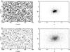 |
Fig. 1 PSF treatment applied to stars: in the top-left panel we show the stars ellipticity before the Im2shape deconvolution. The corresponding distribution in terms of ellipticity components (e1, e2) is shown in the top-right panel. Bottom-left panel shows the stars after the deconvolution by the PSF field (see text), and the bottom-right panel the corresponding distribution of (e1, e2), which is more uniformly distributed than before the deconvolution. Both left panels shows in red the scale corrsponding to a semimajor axis of 1′′. |
We first determine the local PSF by looking at the shape of the stars. The resulting PSF field is cleaned and smoothed by looking at the ten nearest stars at each point and removing those that differ by more than 1.5σ from the local average shape. This ensures any jump in the PSF pattern is avoided, e.g. near the masked area. We also exclude objects having an ellipticity greater than 0.2, thus reducing the contamination of the stars catalog by false detections and faint galaxies. The PSF map over the whole field of view is then obtained by averaging the ellipticities of the five nearest stars at each galaxy position. We checked that our Im2shape implementation can recover point-like objects by applying this PSF correction to each star. Figure 2 shows the results of the shape parameters measurements for these stars: the size distribution is dominated by point sources, and the orientation is more uniformly distributed after the PSF correction. Figure 1 also shows that the regular pattern of the stars ellipticities due to the PSF (top row) disappears after the deconvolution.
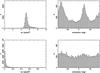 |
Fig. 2 Distribution of the area (left) and orientation (right) of the stars selected in the field of RX J2228.5+2036. The top panels represent the stars before the PSF deconvolution by Im2shape, while the bottom panels show the distribution after deconvolution, with an average size close to point like objects and a uniform orientation of the stars. |
3.2. Validation of the shape measurements with simulated data
To check the performance of our Im2shape implementation, we tested our pipeline on the simulated fields provided by the STEP collaboration (the Shear Testing Programme, Heymans et al. 2006). STEP1 simulations were built to compare the accuracy of different lensing pipelines for ground-based images. They provide a set of images reproducing CFHT-like observations with representative densities of stars and galaxies. These simulations combine several PSF models and shear intensities. We ran our lensing pipeline on each corresponding data set, compared our results to the input configurations and derived an average shear calibration bias and PSF residual.
Our implementation of Im2shape differs slightly from the one proposed by Bridle in the STEP1 simulations: for simplicity and efficiency we fitted both the PSF and the galaxy shapes by a single elliptical Gaussian instead of two concentric ones. This avoids having to deal with two different values of the galaxies ellipticity when measuring the shear profiles. Despite this simplification, our method is very satisfactory because we obtain a calibration bias ⟨m⟩ ≃ −0.1 ± 0.02 and a PSF residual σc ≃ 2 × 10⁻³, a value consistent with shot noise (see Eq. (11) of Heymans et al. 2006). These two values can be compared to the results from other weak lensing methods that are summarized in Fig. 3 of Heymans et al. (2006), so in the present case we introduced an underestimation of the true shear around 10% but with no significant systematics. In the rest of the paper we therefore increase all measures of the shear by a 10% factor before we use them to derive cluster masses.
3.3. Shear radial profiles
When quantifying the shape of a galaxy, we use the complex ellipticity defined by Bonnet & Mellier (1995). It relates the tensor of the galaxy brightness second moments to its shape. Applying the lensing transformation between the source and image planes, one finds the simple relation (Seitz & Schneider 1997): 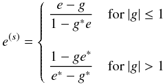 (1)where ∗ denotes the complex conjugate, and e(s) is the complex ellipticity in the source plan and e in the image plan. g is the reduced shear
  (2)which is a nonlinear function of the two lensing functions: the (complex) shear γ and the convergence κ, which is related to the projected mass density.
We assume spherical symmetry of the mass distribution and consider that unlensed galaxies are randomly oriented on the sky plane. This is observationally confirmed since the distribution of the field galaxy ellipticities can be fitted by a Gaussian  (Tyson & Seitzer 1988; Brainerd et al. 1996). In the weak-lensing approximation (i.e. κ ≪ 1), we get an unbiased estimator of the reduced shear by averaging the shape of background galaxies in concentric annuli around the cluster center. Spherical symmetry also implies that the averaged radial component of the shear vanishes, i.e. ⟨e⊥⟩ = 0, while the tangential component of the lensed galaxies traces the reduced shear ⟨e//⟩ = g. We also assume that ⟨e(s)⟩ = 0 with an intrinsic dispersion σe ≈ 0.25. The measure of this averaged tangential component ⟨e//⟩ at different distances provides a reduced shear profile g(r), which is used to recover the total mass of the deflector.
We fix the center of the lens at the position of the brightest galaxy (BCG). The nonparametric mass reconstructions of the cluster sample that will be presented in Paper II show separations between the cluster mass center and the location of the BCG smaller than 30′′ for all clusters except the most disturbed ones or those with a low S/N mass reconstruction. Real shifts between the BCG and the mass center are expected, especially in the most massive dark matter haloes or in nonrelaxed clusters (see e.g. Skibba et al. 2011, for a discussion of the central galaxy paradigm). However, Dietrich et al. (2012) also show with simulated data that for mass reconstructions done with ground-based data, shifts are observed with a median value of 1′ between the true and the reconstructed mass center, so here we cannot reliably disentangle artifacts in the 2D mass reconstructions from real shifts between the BCG and the mass center. Moreover, given the redshifts and mass of the clusters, small miscenterings only disturb the central data points in the shear profile. As discussed in Mandelbaum et al. (2010), excluding the central parts of the profiles in the fitting procedure reduces the underestimation of the mass because of miscentering. Basic simulations (lensing a typical catalog of sources by a cluster representative of the sample in terms of mass and redshift) show that our fitting methodology gives consistent masses within their error bars up top miscentering of 1′. Therefore we consider that the BCG is a good estimator in our case of the actual mass center and that this assumption does not have any consequence on the total mass determination.
Shear profiles are built in nonoverlapping logarithmic annuli with rout = 1.2rin, in order to have similar S/N in each bin. Thanks to the wide field images taken with Megacam, we are able to measure shear profiles up to 600 to 800′′ from the BCG. We limit the fit of the shear profile in the central region to an inner radius set at 25′′ (which roughly corresponds to the Einstein radius of the clusters) except for four clusters that present a shear signal that is too disturbed in the central part. In these cases, the limit is fixed to the radius where the signal becomes significantly positive. This inner limit reduces the impact of miscentering and avoids complications due to the nonlinearity of the reduced shear with mass density. It also avoids the noise induced by galaxies whose shape is badly estimated because they are too close to bright cluster galaxies (e.g. Cypriano et al. 2004).
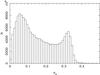 |
Fig. 3 Distribution of the errors on the galaxies ellipticity estimator given by Im2shape (here for RX J2228.5+2036). The minimum of the histogram is reached for an uncertainty σe ~ 0.25. This value gives a natural cut to clean up the catalogs of galaxies used to measure the shear profiles. |
Within these limits, 10 to 15 data points are available in the shear profile (see Figs. 10–20). To improve the statistical weight of the results, we chose to construct 25 shifted profiles by moving the position of the lower bound of the first bin by 1/25 of its width. This allows reduction of the sampling effects in the first points of the profile where the averaged tangential ellipticity can significantly change according to the way the galaxies are binned. Each of these 25 profiles are fitted using a standard χ2 minimization. Because the distribution of field galaxies ellipticity is Gaussian, e.g. Brainerd et al. (1996), the likelihood follows Gaussian statistics. By doing so, we limit the correlation that would arise with overlapping bins.
To improve the shear estimator, we weighted the average value of the tangential component of the galaxies’ ellipticity with the inverse of the ellipticities distribution variance  :
:  (3)where σ// is the quadratic sum of the errors (σe1,σe2) given by Im2shape for each object and the intrinsic dispersion of the galaxies ellipticities σint = 0.25. We also cut our catalogs of galaxies by limiting the uncertainties returned by Im2shape to (σe1,σe2) < 0.25. This value corresponds to the average minimum in the uncertainty distributions (Fig. 3), the objects above this threshold being most likely false detections or very faint/small galaxies. Also thanks to our weighting scheme, removing them does not have any consequences on the final mass estimates (see Cypriano et al. 2004, for details).
To assess the uncertainties on the best fit parameters, we proceed as follows. Assuming that the measures gi have a Gaussian uncertainty σi (although the distribution of the errors appear to be highly non-Gaussian in Fig. 3, ellipticities for each galaxy generated by Im2shape have a Gaussian distribution), we generated 1000 Monte Carlo draws on each of the 25 shifted shear profiles, and applied the χ2 procedure. We then obtain 25 000 values of the best fit parameters. The mode of the resulting distribution gives the most likely solution along with the 1, 2, and 3σ assymetric errors.
3.4. Normalization of the shear profiles
To limit the contamination of the source catalogs, we introduced several magnitude and color cuts, which are discussed in details in Paper II. In summary, we limit the magnitude range to 21–m_comp+0.5 in r′ and remove all objects located within a color-band defined by the bright ellipticals red sequence up to mr = 23. This reduces the galaxy density by about one third even if some contamination by bluer galaxies remains. To overcome this problem, we followed the method proposed by Hoekstra (2007), which assumes that the number density of cluster members simply decreases with radius as 1/r. We adjusted the normalization by fitting the profile of galaxies excess relative to the background level and we corrected the measured shear according to the distance to the cluster center (Fig. 4). Since the richness of a cluster scales with its mass, this contamination is higher for more massive objects, so we applied the renormalization procedure for each cluster instead of using an average correction as in Hoekstra (2007).
 |
Fig. 4 Density profile of the background galaxies used for the fit of the shear profile in the field of MS 1621.5+2640. Despite the removal of the galaxies within the red sequence, a substantial fraction of cluster members remain. The density profile is fit (dashed red line) to give the boosting factor applied to the shear profile. |
Photometric redshift information is also needed to correct for two effects that change the normalization of the shear profiles. The first one is an assessment of the fraction of foreground galaxies in the catalogs and the second is the determination of the average redshift distribution of the background sources. To get a reliable faint-galaxy redshift distribution, we used the photometric redshifts of galaxies in reference fields, neglecting the cosmic variance between different fields (Cypriano et al. 2004; Hoekstra 2007; Limousin et al. 2009; Oguri et al. 2009). Observations in the CFHTLS Deep fields obtained with the same instrument form the ideal data set for our study (Gavazzi & Soucail 2007). They are much deeper than the present observations, so we can consider that their catalogs are complete up to our magnitude limit. We used the photometric redshifts determined with the HyperZ software (Bolzonella et al. 2000). They were calibrated and validated by comparison with spectroscopic redshifts obtained in the VVDS D1 field (Le Fèvre et al. 2005) and in the Growth Deep survey (Weiner et al. 2005). Once our photometric selection criteria were applied to the CFHTLS catalogs, we obtained a redshift distribution that is supposed to be representative of the catalogs we use for the weak lensing analysis.
We used this distribution of photometric redshifts to determine the strength of the shear signal via the geometrical factor β(zL,zS) = DLS/DOS where DLS is the angular-diameter distance between the lens and the source and DOS the distance to the source. Both the convergence κ and the shear γ can be rewritten as (Hoekstra et al. 2000)  (4)where βs = β/β∞ and β∞,γ∞,κ∞ are the corresponding functions for a source at infinity. In the weak-lensing approximation, g ≈ γ, the redshift dependence of the signal is easy to take into account since the average reduced shear simply equals its value taken with the average geometrical factor. For galaxy clusters at low redshift, it is straightforward to replace ⟨β⟩ by the β value of an average redshift zs, usually set to one (Okabe & Umetsu 2008; Radovich et al. 2008). In the present case, the geometrical factor varies significantly with the sources redshifts so we computed the factor ⟨β(z)⟩ for the whole distribution of field galaxies. We account for the contamination by foreground galaxies given our selection criteria by setting β(zphot < zcluster) = 0 (values in a range of 20% to 30% depending on the cluster). Such an approach is only valid in the weak-lensing regime because of the nonlinearity of the reduced shear with β (see e.g. Seitz & Schneider 1997; Hoekstra et al. 2000). However, as with remove the central parts from the fits, we expect these ⟨β(z)⟩ to be a good approximation. The averaged geometrical factors are given in Table 2, along with the effective redshift defined as β(zeff) = ⟨β(z)⟩.
Summary of the weak lensing analysis.
4. Weak-lensing masses
4.1. Mass models
We restrict our analysis to the two mostly used parametric mass models: the singular isothermal sphere (SIS) and the NFW model (Navarro et al. 1995). The SIS mass model is the simplest one for describing a relaxed massive sphere with a constant and isotropic velocity dispersion σv. The mass density profile writes as  and simple expressions are derived for the lensing functions γ(r) = κ(r) = RE/2r where the Einstein radius scales as
  . This mass model is a poor description of the actual mass distribution of clusters, so the fitting results of this mass model is not used to derive the total clusters mass in the rest of this work. However, it allows easy comparisons with other mass estimators, such the dynamical analysis of the galaxies members that are also characterized by a velocity dispersion σv. It also provides an estimate of the Einstein radius RE, which can be compared to results from strong-lensing analysis. This quantity requires an estimate of the geometrical factor to be converted from σv. Values given in Table 2 are derived using a source redshift zs = 2, which leads to radii in the range 20″−40″. These values are not directly estimated from the signal in the central part as done in strong lensing analysis but derived from the fit of the weak lensing shear profile.
The NFW mass profile (Navarro et al. 1997, 2004) was introduced to model the mass distribution of a cold dark matter halo formed in a gravitational scenario of structures formation. It involves a shape parameter, the concentration c, and a normalization parameter often expressed as the scale radius rs:  where ρc is the critical mass density of the Universe at the redshift of the cluster, and δc a dimensionless factor related to the contrast density of a virialized dark matter halo
  by
by  We also define R200 = c rs, often called the virial radius, and the mass enclosed within this radius
  and Δ = 200 roughly corresponds to the virialized part of clusters. X-ray studies more often make use of Δ = 500, a density contrast more easily reached by the X-ray detection. Given the above relations, it is straightforward to analytically switch masses and radii from one Δ value to another.
With two free parameters, the NFW model provides more freedom to adjust the mass profile of galaxy clusters. However, there is a well-known degeneracy between the total mass M200 and the concentration parameter c when fitting the shear profile in the weak lensing regime. This comes from a lack of information on the mass distribution near the cluster center. The observed c − M degeneracy shows a much steeper slope than the theoretical one (Okabe et al. 2010a), and only a combination of strong and weak lensing can raise it and provide useful constraints on the concentration parameter. In the present case, with no strong lensing modeling of all the clusters in the sample, we decided to fix the concentration parameter and only fit the total mass M200. Indeed for most of the clusters, the fit of both parameters leads to unrealistic values of c, either larger than 20 or, in most cases, fixed to the lower limit of the fit c = 2. Since a low concentration is associated to a lower mass when fitting a given shear profile, this leads to the apparent bias observed in Fig. 5, which is only an artifact due to poor constraints in the central parts of the shear profiles. For a more secure mass estimator we therefore fixed the concentration parameter c to a canonical value for massive clusters, c200 = 4, and fit the mass profile with only one free parameter.
It is interesting to note that the ratio between the NFW mass M200 and the SIS mass integrated within R200 is close to one for the whole sample:  . This reflects the fact that in this study of high redshifts clusters of galaxies, weak lensing data only provide constraints on the total mass on large scales. It cannot efficiently constrain the radial mass profile contrary to clusters at lower redshifts where some disagreements are found between the two mass models (Okabe et al. 2010a).
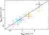 |
Fig. 5 Comparison between the total mass M200 (expressed in units of |

In summary, we have in hand the results of the fit by an SIS profile (σv and RE) for each cluster as well as those by an NFW profile (M200 and R200). The mass and the radius taken at Δ = 500 are also computed for comparison with the results of the X-ray analysis. All these values are given in Table 2. Because we are interested here in calibrating the scaling relation and scatter of individual clusters around the best fits, we have not included the systematic uncertainty owing to the projection effects of the large-scale structures. This effect should be less than 10% for rich clusters at intermediate redshifts (Hoekstra 2001). We also did not include the error on the geometrical factor ⟨β⟩. Its value varies in a range 3−6% depending on the cluster when the different CFHTLS Deep fields are used to estimate it. Moreover, in the present case, these two quantities are second-order effects, and the main source of uncertainties remains the intrinsic ellipticity of the lensed galaxies (e.g. Hoekstra 2007).
4.2. Comparison of the X-ray and weak lensing masses
Raw XMM-Newton data were processed as described in Pointecouteau et al. (2005) and Pratt et al. (2007). As for the REXCESS sample (Croston et al. 2008), surface brightness profiles were PSF-corrected, deprojected, and converted to 3D density profiles using the nonparametric method described in Croston et al. (2006). The 2D temperature profiles were extracted from XMM-Newton spectroscopy as described in Pratt et al. (2010). The 3D profiles were recovered assuming analytical functions taking into account the PSF mixing effects and weighting the contribution of temperatures in various rings. A Monte Carlo procedure was used to compute the errors (Arnaud et al. 2010). The hydrostatic mass equation was then applied to the density and temperature profiles and to their logarithmic gradients to derive the observed mass profile for each cluster. Again a Monte Carlo method was applied to determine the errors on each point, taking overconstraints on the 3D profile imposed by the use of a parametric model into account. Observed mass profiles were finally fitted with an NFW profile, thereby constraining the shape and the normalization parameters, i.e. c500 and M500.
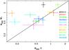 |
Fig. 6 Masses obtained with the weak lensing analysis (y-axis) versus the hydrostatic equilibrium masses obtained with the X-ray analysis (x-axis). All masses are given in units of |

Figure 6 shows the comparison between the weak lensing and the hydrostatic equilibrium masses derived from the X-ray data for the eleven clusters. The comparison is made at a density contrast Δ = 500 to avoid any extrapolation of the X-ray data. The weak lensing masses M200 are simply converted into M500 by assuming a concentration parameter c200 = 4. This means that we are not comparing weak lensing and hydrostatic masses evaluated in the same physical radius. We are instead focusing here on a raw comparison between fitting results.
Over the whole sample, we almost reach a 1σ agreement between the two mass estimators since seven clusters (i.e. ~64%) have compatible masses within their 1σ interval of individual uncertainties, with small scatter and no strong systematics, Fig. 7. With the eleven clusters, we obtain an average mass ratio 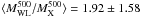 . Removing MS 1241.5+1710 that is almost 3σ away from this average ratio, we find ⟨MWL/MX⟩ = 1.49 ± 0.75, a much less scattered value. We recover here the “classical” result that is a moderate excess for the weak lensing masses.
Similar studies were previously done on clusters at lower redshifts (Zhang et al. 2008; Mahdavi et al. 2008; Zhang et al. 2010), but it is the first time we show this kind of comparison in such a high redshift range. Unfortunately, the weak lensing mass profiles are not constrained enough to allow a more detailed study of the variation with radius of the mass ratio MWL/MX. A combination with strong lensing information would be needed to overcome this difficulty. It will be explored in a forthcoming paper for the EXCPRES clusters for which strong lensing features are detected (4 out of the 11 clusters).
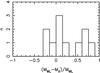 |
Fig. 7 Relative difference distribution between the weak lensing masses and the X-ray masses for the 11 clusters of our sample. Masses are given at the density contrast Δ = 500. |
For the four outliers identified in Fig. 6, their individual properties will be presented in Paper II. However it remains difficult to fully understand on a case by case basis why these clusters show such discrepancies. It certainly results from the mixed effect of intrinsic physical departures from hydrostatic equilibrium and the limited quality of the lensing data. Some differences are also statistically expected in unbiased samples of clusters and can be characterized with numerical simulations (Meneghetti et al. 2010). However, because of the limited size of the sample, we did not separate dynamically perturbed clusters from the relaxed one to try highlighting variations in the normalization and scatter of the MWL − MX relation.
Summary of the fitting results for the scaling relations (M/M0) = A × (Obs./Obs.0)α.
5. Mass-observable correlations
5.1. Methodology
Because both masses and observables have uncertainties with possible correlations (e.g. the richness depends on R200 and thus on the total mass), a simple χ2 minimization cannot be used to calibrate scaling relations. Moreover, we expect to have an intrinsic dispersion around the main scaling relation, which needs to be included and evaluated, so we preferred to perform a linear regression using the orthogonal BCES estimators (Bivariate Correlated Errors and intrinsic Scatter, Akritas & Bershady 1996). This approach has already been used by several groups for calibrating mass-observable scaling relations (Morandi et al. 2007; Pratt et al. 2009), which are expected to be characterized by power laws and so fitted by linear relations y = ax + b in the log-log plan. For each relation, both variables are normalized by a pivot close to their mean. This insures that the logarithmic slope and normalization of the relation are nearly independent parameters.
Once the best fit of the correlation is obtained, the total dispersion over the N points,  (5)equals the quadratic sum of the statistical dispersion σstat and the intrinsic one σint, which thus can be expressed as
 ![\begin{equation} \sigma_{\rm int}^{2}=\frac{1}{N-2}\sum_{i=1}^{N}\left[(y_{i}-\alpha x_{i}-B)^{2}-\frac{N-2}{N}\left(\sigma_{y_{i}}^{2}+\alpha^{2}\sigma_{x_{i}}^{2}\right)\right] . \end{equation}](/articles/aa/full_html/2012/10/aa18973-12/aa18973-12-eq266.png) (6)For each relation, we also estimated the Spearman correlation coefficient ρ:
(6)For each relation, we also estimated the Spearman correlation coefficient ρ:  (7)where di is the ranking difference of the ith sorted mass and observable vector. This correlation coefficient shows the monotonic degree of the relation between the two variables (ρ = −1 for a strictly decreasing relation, ρ = + 1 in the opposite case). Compared to the classical Pearson coefficient, the Spearman coefficient does not depend on the slope of the correlation. Such a coefficient has been used in similar studies to quantify the strength of a correlation, e.g. Lin et al. (2004).
5.2. Optical scaling laws
First, we compared the weak lensing mass M200 to the optical richness N200. We defined N200 as number of galaxies within R200 that belong to the cluster red sequence (the precise definition will be presented in Paper II). We kept only the brightest members with L < 0.4L⋆, where L⋆ is derived from the values of Ilbert et al. (2005) and according to the cluster redshifts. Richnesses are corrected from the background contamination but are not corrected from any luminosity cut or any color selection. The aim is to remain consistent with previous studies that focus on the bright elliptical cluster galaxies.
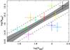 |
Fig. 8 Mass-richness scaling relation calibrated with the NFW lensing masses M200. The black line shows the best BCES orthogonal fit. The region limited by the two dashed lines corresponds to the intrinsic dispersion of the galaxy clusters around the best fit. The shaded area gives the statistical 1σ uncertainty given by the best fit parameters. |
The BCES calibration of this M200 − N200 relation, given in Table 3 (with masses in units of  and richnesses normalized to 80), presents a correlation with a logarithmic slope α = 1.04 ± 0.38 (Fig. 8). Despite a rather large uncertainty, the slope is very close to 1, in agreement with the simplest model of structures formation (Kravtsov et al. 2004). The uncertainties of the BCES fit are dominated by the intrinsic dispersion due to the limited size of the cluster sample and increased by one outlier, RX J2228.5+2036. These results are coherent with previous studies conducted at lower redshifts (Becker et al. 2007; Johnston et al. 2007; Reyes et al. 2008; Rykoff et al. 2008; Mandelbaum et al. 2008; Rozo et al. 2009). We also compared the X-ray masses with the cluster richnesses. This leads to a correlation with a slope α = 1.14 ± 0.18. In addition, we also looked at a possible correlation between the mass and the richness evaluated in a given physical radius. In practice, we used the richness determined within 1 Mpc (roughly equal to 0.5R200). The BCES estimator gives a slope α = 1.60 ± 0.92, a result with a very large uncertainty that is useless with the present data.
To compare these different approaches, we computed the relative error R = |(MWL − Mproxy)/MWL| averaged over the sample of clusters after removing the main outlier RX J2228.5+2036. The M − N200 relation leads to R = 0.27, while we find R = 0.41 with the M − N1 Mpc relation. Even if the conversion between richness and mass within a fixed aperture is less physical than the use of the virial radius R200, we show here that it is still acceptable. Clearly the uncertainties in the scaling relations are dominated by the intrinsic dispersion more than by the choice of the working radius (see also Andreon & Hurn 2010). Accurate determination of R200 is a second-order effect, and using a simple fixed aperture for the measure of the cluster richness can already lead to a correct mass proxy. This is particularly true since our sample covers a restricted interval in both mass and redshift, so the fixed aperture is not far from a fixed density contrast.
Second, we tested the relationship between mass and optical luminosity. The M − L correlation gives a roughly constant mass-to-light ratio as the BCES estimator returns a slope α = 0.95 ± 0.37 (see Table 3 with masses in units of and luminosities normalized to  ). To be consistent with other similar works, we did not correct the total luminosities from incompleteness. Our catalogs are limited to 0.4 L⋆, and a correcting factor of ~1.6 should be included to get the total luminosity, assuming a standard Schechter luminosity function. This is done in Paper II, which discusses the M/L ratio of the clusters in detail. The correlation between X-ray masses and optical luminosities gives α = 1.20 ± 0.20, a value also compatible with a constant mass-to-light ratio. As for the M − N relation, the calibration with the X-ray masses gives a smaller intrinsic dispersion.
Previous studies tend to find a slope in the M − L relation that is slightly larger than one (Lin et al. 2004; Popesso et al. 2005; Bardeau et al. 2007; Reyes et al. 2008). This tendency is predicted by some of the semi-analytical models of galaxy formation, at least for massive clusters (Marinoni & Hudson 2002) in which the star formation efficiency can be inhibited by the long cooling times of hot gas on high-mass scales. Merging processes and galaxies interactions can also affect the luminosity of galaxies and are more efficient in massive clusters. But because of the narrow mass range covered by our cluster sample, it is difficult to draw firm conclusions on any possible variation in the M/L ratio with mass. It would be necessary to add galaxy groups in the sample, although accurate mass determinations are quite difficult for low-mass structures.
Moreover, the complex method of determining the value of R200 represents a problem for estimating L200, so we repeated the same procedure as described above and compared the masses with luminosities integrated inside a 1 Mpc radius. We also calculated the average relative errors on the mass. We obtain R = 0.47 for masses derived from the M − L1 Mpc relation, while we get R = 0.33 when we use the M − L200 relation. Again, the intrinsic dispersion is the main source of uncertainties, since the precise determination of R200 is a second-order effect.
5.3. X-ray scaling laws
We focus here only on scaling laws fitted with the weak lensing masses taken at Δ = 200. The calibration of the LX − M relation has been the subject of many studies, mainly at low redshifts. Mass estimators are usually derived from X-ray data (Markevitch 1998; Arnaud et al. 2002; Reiprich & Böhringer 2002; Popesso et al. 2005; Morandi et al. 2007; Pratt et al. 2009; Vikhlinin et al. 2009). Several attempts to use weak lensing masses have also been proposed more recently (Hoekstra 2007; Bardeau et al. 2007; Rykoff et al. 2008; Leauthaud et al. 2010; Okabe et al. 2010b). Most these studies converge towards a power law that differs from the relation expected in the hierarchical scenario of structure formation where the X-ray luminosity scales with the mass as  . The Fz factor stands for the evolution of the scaling relation and reduces to h(z), the reduced Hubble constant, for models of structures formation based only on gravitation and assuming a fixed density contrast to derive masses (Voit 2005).
Several processes can affect the properties of a cluster, generating both an intrinsic dispersion around the expected LX − M relation and a break of self-similarity. Most previous studies point towards a slope that is slightly steeper than the expected one, i.e. α = 1.6–1.8 instead of 4/3. The intrinsic dispersion is found to be quite large, up to almost 50% (Reiprich & Böhringer 2002). However, it appears that, when cool cores are removed, this intrinsic dispersion is smaller (Allen 1998; Markevitch 1998; Voit et al. 2002; Maughan 2007; Pratt et al. 2009). Indeed, the X-ray luminosity is strongly affected by the physical mechanisms ruling the baryonic content of clusters (pre-heating, radiative cooling, feedback of supernovae and active galactic nuclei, etc.), and so is the LX − M with respect to the simplest gravitational model. These processes are modeled in up-to-date numerical simulations that combine the gravitational evolution of dark matter structures with the hydrodynamical behavior of the intracluster gas (Borgani et al. 2004; Kay 2004; Borgani 2008). These simulations also seem to favor a slope of the LX − M relation that is steeper than the canonical one.
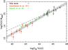 |
Fig. 9 Weak-lensing masses versus X-ray luminosities using the EXCPRES clusters (black boxes) combined with the stacked clusters and groups of Rykoff et al. (2008) (green circles) and of Leauthaud et al. (2010) (red crosses). The solid lines show the best BCES fit and the corresponding intrinsic dispersion for the three data sets. For comparison, the BCES best fit obtained with only the EXCPRES weak lensing subsample is plotted (dashed line). |
The results of the BCES estimator for the  relation are presented in Table 3 (with masses in units of
  and X-ray luminosities in units of
  ). Although our LX measurements do not purely equate LX,200 (see Table 1), our best fit relation is in good agreement with previous works since we find a slope α = 2.06 ± 0.44. Despite a strong correlation, we also observe a large scatter around the best fit with σint = 0.19.
These encouraging results should nonetheless be taken with caution because our subsample of the EXCPRES clusters was designed to keep only the most luminous clusters in the sample. It therefore covers a limited range in X-ray luminosity. To explore a broader range, we combined this sample with clusters from two studies: (i) the COSMOS galaxy groups analyzed in Leauthaud et al. (2010) and (ii) the maxBCG galaxy groups and clusters presented in Rykoff et al. (2008, Fig. 9). Both use stacks of objects with similar richness to improve the statistics of the shear profiles for low-mass objects. Their X-ray luminosities are also stacked within R200 apertures, whereas our values of the luminosities are computed within the detection radius (see Table 1). However, we checked that the ratio between Rdet and R200 for our sample is ~0.9 on average. We therefore consider that the present values are close enough to the values within R200, thus allowing us to compare and combine them with the aforementioned works. This combination of the three data sets allows covering an extended range in mass and luminosity. We fit them simultaneously and the best fit relation gives a slope of α = 1.57 ± 0.07. This slope is less than from our data alone, but still in disagreement with the hierarchical prediction of 4/3. The intrinsic dispersion stays roughly unchanged over the combined sample.
Although it is not nowadays often used as a mass proxy, we then checked the MWL − T relation. We derived a slope of α = 1.33 ± 0.42, a value compatible with the self-similar prediction of 1.5 within the 1σ limit (see Table 3 with masses in units of and temperatures normalized to 5 keV). This weak-lensing calibration is compatible with those by Hoekstra (2007) and Okabe et al. (2010b), who derive slopes of α = 1.34 ± 0.29 and α = 1.49 ± 0.58 respectively.
We also computed the average relative error R between the weak-lensing masses and the mass proxies determined with X-ray data. The LX − M relation gives R = 0.28, and the M − T leads to R = 0.31. These two values are close to those previously obtained for the M − N and M − L correlations with optical data.
6. Summary and conclusions
In this paper we have provided for the first time a thorough weak lensing analysis of a sample of 11 galaxy clusters (a sub-sample of the EXCPRES sample – Arnaud et al., in prep.) in a relatively high-redshift range, 0.4 < z < 0.6. We conducted a careful validation of our weak lensing pipeline, thanks in particular to the STEP simulations that allowed us to recalibrate our shear measurements. The shear profiles were fitted with an NFW profile with a fixed concentration parameter c200 = 4. This is due to the lack of good constraints on the shear profile near the center so only the total mass M200 is a reliable measure. These weak lensing masses were compared to the X-ray masses derived from XMM-Newton data. Over the eleven clusters, we find a good match between these two mass estimators for seven clusters while we found four outliers, thus having almost 1σ agreement in the two methods. Such results are consistent with other similar studies performed for lower redshift samples.
The primary goal of this study was to look for correlations between the total mass of galaxy clusters and several baryonic tracers. In our sample of massive clusters, we found that the total mass is proportional to the optical richness of galaxies. This result is in good agreement with previous works at lower redshifts (Becker et al. 2007; Johnston et al. 2007; Reyes et al. 2008; Rykoff et al. 2008; Mandelbaum et al. 2008; Rozo et al. 2009). We reached the same conclusion for the correlation between mass and optical luminosity, with a constant ratio M/L, even if the correlation is weaker with a larger intrinsic dispersion. Using XMM-Newton data and the weak lensing masses, we built scaling relations with the X-ray total luminosity and the global spectroscopic temperature. Although weakly constrained due to limited coverage of the mass range, both correlations give results in good agreement with previous studies: (i) the mass-luminosity relation presents a non-self-similar slope, larger than expected from a purely gravitational model of structure formation; (ii) the mass-temperature relation is roughly compatible with the hierarchical prediction. We have extended our investigation of the LX − M relation by combining our cluster sample with two samples of groups and clusters for which weak lensing masses were obtained (Rykoff et al. 2008; Leauthaud et al. 2010). The resulting LX − M200 relation covers nearly two decades in mass and displays a regular shape with a well constrained slope.
Even if the limited size of our sample and its reduced mass range coverage allowed us to only probe the high end of the mass distribution of clusters, we demonstrated the synergy with the X-ray measurements (i.e., mass, luminosity, and temperature). More specifically, we confirmed that the scaling relations with the lensing mass proxy are already in place at z ~ 0.5, with, at first order, no significant departures from the same relations at lower redshift (assuming a self-similar evolution). The limited quality of the lensing data for our sample restricts the added value of a joint analysis, but the weak lensing and X-ray coverage of cluster proved to be complementary. Indeed X-ray data allows efficiently probing of the central regions out to about R500. Beyond this radius the X-ray brightness rapidly drops, whereas the weak-lensing signal picks up to characterize the outer parts of massive halos. A perspective work would be to investigate the strong lensing signal (see Table1) of each cluster in our sample, in order to perform a full lensing analysis from the inner part (with the strong lensing signal) to the outer parts (with the weak lensing signal). This would provide a coherent mass proxy estimator to be compared directly with X-ray and dynamical proxies.
Finally, in the perspective of large optical surveys such as the Euclid space mission, self-calibrated mass proxies will be needed for any full scientific exploitation of the mission. The M − N relation is an obvious candidate, whose tight calibration will require validation against other relations and mass proxies, such as the X-ray mass. The M − N relation we provide in this paper is an early result in the redshift range 0.4 < z < 0.6. It illustrates the difficulty constraining this particular scaling relation. Provided the N estimator is made as universal as possible, which can be a nontrivial task, this relation is promising in the framework of optical surveys.
Acknowledgments
We wish to thank Roser Pello for many fruitful discussions. She provided the catalogs of photometric redshifts built from the CFHTLS Deep fields that are used in this work. We are grateful to the TERAPIX team who processed part of the data efficiently. We also thank the Programme National de Cosmologie et Galaxies of the CNRS for financial support. M.L. acknowledges the Centre National de la Recherche Scientifique (CNRS) for its support. The Dark Cosmology Centre is funded by the Danish National Research Foundation. The present work is based on observations obtained with XMM-Newton an ESA science mission with instruments and contributions directly funded by ESA Member States and the USA (NASA). This research used the facilities of the Canadian Astronomy Data Centre operated by the National Research Council of Canada with the support of the Canadian Space Agency. This work is based on observations obtained with MegaPrime/MegaCam, a joint project of CFHT and CEA/DAPNIA, at the Canada-France-Hawaii Telescope (CFHT), which is operated by the National Research Council (NRC) of Canada, the Institut National des Science de l’Univers of the Centre National de la Recherche Scientifique (CNRS) of France, and the University of Hawaii.
References
- Akritas, M. G., & Bershady, M. A. 1996, ApJ, 470, 706 [NASA ADS] [CrossRef] [Google Scholar]
- Albrecht, A., Bernstein, G., Cahn, R., et al. 2006, unpublished [arXiv:0609591] [Google Scholar]
- Allen, S. W. 1998, MNRAS, 296, 392 [NASA ADS] [CrossRef] [Google Scholar]
- Andreon, S., & Hurn, M. A. 2010, MNRAS, 404, 1922 [NASA ADS] [Google Scholar]
- Arnaud, M., Aghanim, N., & Neumann, D. M. 2002, A&A, 389, 1 [NASA ADS] [CrossRef] [EDP Sciences] [Google Scholar]
- Arnaud, M., Pratt, G. W., Piffaretti, R., et al. 2010, A&A, 517, A92 [NASA ADS] [CrossRef] [EDP Sciences] [Google Scholar]
- Bahcall, N. A., & Cen, R. 1992, ApJ, 398, L81 [NASA ADS] [CrossRef] [Google Scholar]
- Bardeau, S., Kneib, J.-P., Czoske, O., et al. 2005, A&A, 434, 433 [NASA ADS] [CrossRef] [EDP Sciences] [Google Scholar]
- Bardeau, S., Soucail, G., Kneib, J.-P., et al. 2007, A&A, 470, 449 [NASA ADS] [CrossRef] [EDP Sciences] [Google Scholar]
- Bartelmann, M., & Schneider, P. 2001, Phys. Rep., 340, 291 [NASA ADS] [CrossRef] [Google Scholar]
- Becker, M. R., McKay, T. A., Koester, B., et al. 2007, ApJ, 669, 905 [NASA ADS] [CrossRef] [Google Scholar]
- Böhringer, H., Schuecker, P., Pratt, G. W., et al. 2007, A&A, 469, 363 [NASA ADS] [CrossRef] [EDP Sciences] [Google Scholar]
- Bolzonella, M., Miralles, J.-M., & Pelló, R. 2000, A&A, 363, 476 [NASA ADS] [Google Scholar]
- Bonnet, H., & Mellier, Y. 1995, A&A, 303, 331 [NASA ADS] [Google Scholar]
- Borgani, S. 2008, in A Pan-Chromatic View of Clusters of Galaxies and the Large-Scale Structure, eds. M. Plionis, O. López-Cruz, & D. Hughes, Lect. Notes Phys. (Berlin: Springer Verlag), 740, 287 [Google Scholar]
- Borgani, S., Murante, G., Springel, V., et al. 2004, MNRAS, 348, 1078 [NASA ADS] [CrossRef] [Google Scholar]
- Bradač, M., Schneider, P., Lombardi, M., & Erben, T. 2005, A&A, 437, 39 [NASA ADS] [CrossRef] [EDP Sciences] [Google Scholar]
- Brainerd, T. G., Blandford, R. D., & Smail, I. 1996, ApJ, 466, 623 [NASA ADS] [CrossRef] [Google Scholar]
- Bridle, S., Gull, S., Bardeau, S., & Kneib, J.-P. 2002, in Proc. Yale Cosmology Workshop: The Shapes of Galaxies and their Dark Halos, ed. N. Priyamvada (World Scientific) [Google Scholar]
- Buote, D. A., Gastaldello, F., Humphrey, P. J., et al. 2007, ApJ, 664, 123 [NASA ADS] [CrossRef] [Google Scholar]
- Croston, J. H., Arnaud, M., Pointecouteau, E., & Pratt, G. W. 2006, A&A, 459, 1007 [NASA ADS] [CrossRef] [EDP Sciences] [Google Scholar]
- Croston, J. H., Pratt, G. W., Böhringer, H., et al. 2008, A&A, 487, 431 [NASA ADS] [CrossRef] [EDP Sciences] [Google Scholar]
- Cypriano, E. S., Sodré, Jr., L., Kneib, J., & Campusano, L. E. 2004, ApJ, 613, 95 [NASA ADS] [CrossRef] [Google Scholar]
- Dietrich, J. P., Böhnert, A., Lombardi, M., Hilbert, S., & Hartlap, J. 2012, MNRAS, 419, 3547 [NASA ADS] [CrossRef] [Google Scholar]
- Gavazzi, R., & Soucail, G. 2007, A&A, 462, 459 [NASA ADS] [CrossRef] [EDP Sciences] [Google Scholar]
- Haiman, Z., Mohr, J. J., & Holder, G. P. 2001, ApJ, 553, 545 [NASA ADS] [CrossRef] [Google Scholar]
- Heymans, C., Van Waerbeke, L., Bacon, D., et al. 2006, MNRAS, 368, 1323 [NASA ADS] [CrossRef] [Google Scholar]
- Hoekstra, H. 2001, A&A, 370, 743 [NASA ADS] [CrossRef] [EDP Sciences] [Google Scholar]
- Hoekstra, H. 2003, MNRAS, 339, 1155 [NASA ADS] [CrossRef] [Google Scholar]
- Hoekstra, H. 2007, MNRAS, 379, 317 [NASA ADS] [CrossRef] [Google Scholar]
- Hoekstra, H., Franx, M., & Kuijken, K. 2000, ApJ, 532, 88 [NASA ADS] [CrossRef] [Google Scholar]
- Ilbert, O., Tresse, L., Zucca, E., et al. 2005, A&A, 439, 863 [NASA ADS] [CrossRef] [EDP Sciences] [Google Scholar]
- Johnston, D. E., Sheldon, E. S., Wechsler, R. H., et al. 2007, unpublished [arXiv:0709.1159] [Google Scholar]
- Kaiser, N. 1986, MNRAS, 222, 323 [NASA ADS] [CrossRef] [Google Scholar]
- Kay, S. T. 2004, MNRAS, 347, L13 [NASA ADS] [CrossRef] [Google Scholar]
- Kneib, J., Hudelot, P., Ellis, R. S., et al. 2003, ApJ, 598, 804 [NASA ADS] [CrossRef] [Google Scholar]
- Kravtsov, A. V., Berlind, A. A., Wechsler, R. H., et al. 2004, ApJ, 609, 35 [NASA ADS] [CrossRef] [Google Scholar]
- Kravtsov, A. V., Vikhlinin, A., & Nagai, D. 2006, ApJ, 650, 128 [NASA ADS] [CrossRef] [Google Scholar]
- Lau, E. T., Kravtsov, A. V., & Nagai, D. 2009, ApJ, 705, 1129 [NASA ADS] [CrossRef] [Google Scholar]
- Le Fèvre, O., Vettolani, G., Garilli, B., et al. 2005, A&A, 439, 845 [NASA ADS] [CrossRef] [EDP Sciences] [Google Scholar]
- Leauthaud, A., Finoguenov, A., Kneib, J., et al. 2010, ApJ, 709, 97 [NASA ADS] [CrossRef] [Google Scholar]
- Limousin, M., Kneib, J. P., Bardeau, S., et al. 2007a, A&A, 461, 881 [NASA ADS] [CrossRef] [EDP Sciences] [Google Scholar]
- Limousin, M., Richard, J., Jullo, E., et al. 2007b, ApJ, 668, 643 [NASA ADS] [CrossRef] [Google Scholar]
- Limousin, M., Cabanac, R., Gavazzi, R., et al. 2009, A&A, 502, 445 [NASA ADS] [CrossRef] [EDP Sciences] [Google Scholar]
- Lin, Y., Mohr, J. J., & Stanford, S. A. 2004, ApJ, 610, 745 [NASA ADS] [CrossRef] [Google Scholar]
- Mahdavi, A., Hoekstra, H., Babul, A., & Henry, J. P. 2008, MNRAS, 384, 1567 [NASA ADS] [CrossRef] [Google Scholar]
- Mahdavi, A., Hoekstra, H., Babul, A., et al. 2007, ApJ, 664, 162 [NASA ADS] [CrossRef] [Google Scholar]
- Mandelbaum, R., & Seljak, U. 2007, J. Cosmology Astropart. Phys., 6, 24 [NASA ADS] [CrossRef] [Google Scholar]
- Mandelbaum, R., Seljak, U., Hirata, C. M., et al. 2008, MNRAS, 386, 781 [NASA ADS] [CrossRef] [Google Scholar]
- Mandelbaum, R., Seljak, U., Baldauf, T., & Smith, R. E. 2010, MNRAS, 405, 2078 [NASA ADS] [Google Scholar]
- Marinoni, C., & Hudson, M. J. 2002, ApJ, 569, 101 [NASA ADS] [CrossRef] [Google Scholar]
- Markevitch, M. 1998, ApJ, 504, 27 [NASA ADS] [CrossRef] [Google Scholar]
- Maughan, B. J. 2007, ApJ, 668, 772 [NASA ADS] [CrossRef] [Google Scholar]
- Meneghetti, M., Rasia, E., Merten, J., et al. 2010, A&A, 514, A93 [NASA ADS] [CrossRef] [EDP Sciences] [Google Scholar]
- Merten, J., Cacciato, M., Meneghetti, M., Mignone, C., & Bartelmann, M. 2009, A&A, 500, 681 [NASA ADS] [CrossRef] [EDP Sciences] [Google Scholar]
- Metzler, C. A., White, M., & Loken, C. 2001, ApJ, 547, 560 [NASA ADS] [CrossRef] [Google Scholar]
- Morandi, A., Ettori, S., & Moscardini, L. 2007, MNRAS, 379, 518 [NASA ADS] [CrossRef] [Google Scholar]
- Morandi, A., Pedersen, K., & Limousin, M. 2010, ApJ, 713, 491 [NASA ADS] [CrossRef] [Google Scholar]
- Nagai, D., Vikhlinin, A., & Kravtsov, A. V. 2007, ApJ, 655, 98 [NASA ADS] [CrossRef] [Google Scholar]
- Navarro, J. F., Frenk, C. S., & White, S. D. M. 1995, MNRAS, 275, 720 [NASA ADS] [CrossRef] [Google Scholar]
- Navarro, J. F., Frenk, C. S., & White, S. D. M. 1997, ApJ, 490, 493 [NASA ADS] [CrossRef] [Google Scholar]
- Navarro, J. F., Hayashi, E., Power, C., et al. 2004, MNRAS, 349, 1039 [NASA ADS] [CrossRef] [Google Scholar]
- Oguri, M., Hennawi, J. F., Gladders, M. D., et al. 2009, ApJ, 699, 1038 [NASA ADS] [CrossRef] [Google Scholar]
- Oguri, M., Bayliss, M. B., Dahle, H., et al. 2012, MNRAS, 420, 3213 [NASA ADS] [CrossRef] [Google Scholar]
- Okabe, N., & Umetsu, K. 2008, PASJ, 60, 345 [NASA ADS] [Google Scholar]
- Okabe, N., Takada, M., Umetsu, K., Futamase, T., & Smith, G. P. 2010a, PASJ, 62, 811 [NASA ADS] [Google Scholar]
- Okabe, N., Zhang, Y., Finoguenov, A., et al. 2010b, ApJ, 721, 875 [NASA ADS] [CrossRef] [Google Scholar]
- Pointecouteau, E., Arnaud, M., & Pratt, G. W. 2005, A&A, 435, 1 [NASA ADS] [CrossRef] [EDP Sciences] [Google Scholar]
- Popesso, P., Biviano, A., Böhringer, H., Romaniello, M., & Voges, W. 2005, A&A, 433, 431 [NASA ADS] [CrossRef] [EDP Sciences] [Google Scholar]
- Pratt, G. W., Böhringer, H., Croston, J. H., et al. 2007, A&A, 461, 71 [NASA ADS] [CrossRef] [EDP Sciences] [Google Scholar]
- Pratt, G. W., Croston, J. H., Arnaud, M., & Böhringer, H. 2009, A&A, 498, 361 [NASA ADS] [CrossRef] [EDP Sciences] [Google Scholar]
- Pratt, G. W., Arnaud, M., Piffaretti, R., et al. 2010, A&A, 511, A85 [NASA ADS] [CrossRef] [EDP Sciences] [Google Scholar]
- Radovich, M., Puddu, E., Romano, A., Grado, A., & Getman, F. 2008, A&A, 487, 55 [NASA ADS] [CrossRef] [EDP Sciences] [Google Scholar]
- Reiprich, T. H., & Böhringer, H. 2002, ApJ, 567, 716 [NASA ADS] [CrossRef] [Google Scholar]
- Reyes, R., Mandelbaum, R., Hirata, C., Bahcall, N., & Seljak, U. 2008, MNRAS, 390, 1157 [NASA ADS] [CrossRef] [Google Scholar]
- Rozo, E., Rykoff, E. S., Evrard, A., et al. 2009, ApJ, 699, 768 [NASA ADS] [CrossRef] [Google Scholar]
- Rykoff, E. S., Evrard, A. E., McKay, T. A., et al. 2008, MNRAS, 387, L28 [NASA ADS] [Google Scholar]
- Seitz, C., & Schneider, P. 1997, A&A, 318, 687 [NASA ADS] [Google Scholar]
- Skibba, R. A., van den Bosch, F. C., Yang, X., et al. 2011, MNRAS, 410, 417 [NASA ADS] [CrossRef] [Google Scholar]
- Tyson, J. A., & Seitzer, P. 1988, ApJ, 335, 552 [NASA ADS] [CrossRef] [Google Scholar]
- Vikhlinin, A., Kravtsov, A., Forman, W., et al. 2006, ApJ, 640, 691 [NASA ADS] [CrossRef] [Google Scholar]
- Vikhlinin, A., Kravtsov, A. V., Burenin, R. A., et al. 2009, ApJ, 692, 1060 [NASA ADS] [CrossRef] [Google Scholar]
- Voit, G. M. 2005, Rev. Mod. Phys., 77, 207 [NASA ADS] [CrossRef] [Google Scholar]
- Voit, G. M., Bryan, G. L., Balogh, M. L., & Bower, R. G. 2002, ApJ, 576, 601 [NASA ADS] [CrossRef] [Google Scholar]
- Wang, S., Khoury, J., Haiman, Z., & May, M. 2004, Phys. Rev. D, 70, 123008 [NASA ADS] [CrossRef] [Google Scholar]
- Weiner, B. J., Phillips, A. C., Faber, S. M., et al. 2005, ApJ, 620, 595 [NASA ADS] [CrossRef] [Google Scholar]
- White, S. D. M., Navarro, J. F., Evrard, A. E., & Frenk, C. S. 1993, Nature, 366, 429 [NASA ADS] [CrossRef] [Google Scholar]
- Zhang, Y., Finoguenov, A., Böhringer, H., et al. 2008, A&A, 482, 451 [NASA ADS] [CrossRef] [EDP Sciences] [Google Scholar]
- Zhang, Y., Okabe, N., Finoguenov, A., et al. 2010, ApJ, 711, 1033 [NASA ADS] [CrossRef] [Google Scholar]
Appendix A: Additional figures
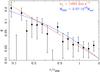 |
Fig. A.1 Reduced shear profile normalized by the virial radius g(r/R200) for the galaxy cluster MS 0015.9+1609. The velocity dispersion σv and the total mass M200 fitted to this profile are given (red curve for the SIS model, blue one for the NFW model). |
All Tables
Summary of the fitting results for the scaling relations (M/M0) = A × (Obs./Obs.0)α.
All Figures
|
Fig. 1 PSF treatment applied to stars: in the top-left panel we show the stars ellipticity before the Im2shape deconvolution. The corresponding distribution in terms of ellipticity components (e1, e2) is shown in the top-right panel. Bottom-left panel shows the stars after the deconvolution by the PSF field (see text), and the bottom-right panel the corresponding distribution of (e1, e2), which is more uniformly distributed than before the deconvolution. Both left panels shows in red the scale corrsponding to a semimajor axis of 1′′. |
| In the text | |
|
Fig. 2 Distribution of the area (left) and orientation (right) of the stars selected in the field of RX J2228.5+2036. The top panels represent the stars before the PSF deconvolution by Im2shape, while the bottom panels show the distribution after deconvolution, with an average size close to point like objects and a uniform orientation of the stars. |
| In the text | |
|
Fig. 3 Distribution of the errors on the galaxies ellipticity estimator given by Im2shape (here for RX J2228.5+2036). The minimum of the histogram is reached for an uncertainty σe ~ 0.25. This value gives a natural cut to clean up the catalogs of galaxies used to measure the shear profiles. |
| In the text | |
|
Fig. 4 Density profile of the background galaxies used for the fit of the shear profile in the field of MS 1621.5+2640. Despite the removal of the galaxies within the red sequence, a substantial fraction of cluster members remain. The density profile is fit (dashed red line) to give the boosting factor applied to the shear profile. |
| In the text | |
|
Fig. 5 Comparison between the total mass M200 (expressed in units of |
| In the text | |
|
Fig. 6 Masses obtained with the weak lensing analysis (y-axis) versus the hydrostatic equilibrium masses obtained with the X-ray analysis (x-axis). All masses are given in units of |
| In the text | |
|
Fig. 7 Relative difference distribution between the weak lensing masses and the X-ray masses for the 11 clusters of our sample. Masses are given at the density contrast Δ = 500. |
| In the text | |
|
Fig. 8 Mass-richness scaling relation calibrated with the NFW lensing masses M200. The black line shows the best BCES orthogonal fit. The region limited by the two dashed lines corresponds to the intrinsic dispersion of the galaxy clusters around the best fit. The shaded area gives the statistical 1σ uncertainty given by the best fit parameters. |
| In the text | |
|
Fig. 9 Weak-lensing masses versus X-ray luminosities using the EXCPRES clusters (black boxes) combined with the stacked clusters and groups of Rykoff et al. (2008) (green circles) and of Leauthaud et al. (2010) (red crosses). The solid lines show the best BCES fit and the corresponding intrinsic dispersion for the three data sets. For comparison, the BCES best fit obtained with only the EXCPRES weak lensing subsample is plotted (dashed line). |
| In the text | |
|
Fig. A.1 Reduced shear profile normalized by the virial radius g(r/R200) for the galaxy cluster MS 0015.9+1609. The velocity dispersion σv and the total mass M200 fitted to this profile are given (red curve for the SIS model, blue one for the NFW model). |
| In the text | |
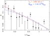 |
Fig. A.2 Same as Fig. A.1 for the cluster MS 0451.6–0305. |
| In the text | |
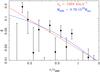 |
Fig. A.3 Same as Fig. A.1 for the cluster RXC J0856.1+3756. |
| In the text | |
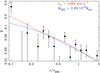 |
Fig. A.4 Same as Fig. A.1 for the cluster RX J0943.0+4659. |
| In the text | |
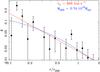 |
Fig. A.5 Same as Fig. A.1 for the cluster RXC J1003.0+3254. |
| In the text | |
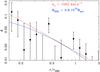 |
Fig. A.6 Same as Fig. A.1 for the cluster RX J1120.1+4318. |
| In the text | |
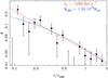 |
Fig. A.7 Same as Fig. A.1 for the cluster RXC J1206.2–0848. |
| In the text | |
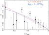 |
Fig. A.8 Same as Fig. A.1 for the cluster MS 1241.5+1710. |
| In the text | |
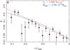 |
Fig. A.9 Same as Fig. A.1 for the cluster RX J1347.5–1144. |
| In the text | |
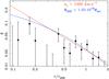 |
Fig. A.10 Same as Fig. A.1 for the cluster MS 1621.5+2640. |
| In the text | |
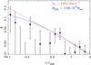 |
Fig. A.11 Same as Fig. A.1 for the cluster RX J2228.5+2036. |
| In the text | |
Current usage metrics show cumulative count of Article Views (full-text article views including HTML views, PDF and ePub downloads, according to the available data) and Abstracts Views on Vision4Press platform.
Data correspond to usage on the plateform after 2015. The current usage metrics is available 48-96 hours after online publication and is updated daily on week days.
Initial download of the metrics may take a while.