| Issue |
A&A
Volume 544, August 2012
|
|
|---|---|---|
| Article Number | L7 | |
| Number of page(s) | 6 | |
| Section | Letters | |
| DOI | https://doi.org/10.1051/0004-6361/201219589 | |
| Published online | 03 August 2012 | |
The first ALMA view of IRAS 16293-2422⋆,⋆⋆
Direct detection of infall onto source B and high-resolution kinematics of source A
1 European Southern Observatory (ESO), Garching, Germany
e-mail: This email address is being protected from spambots. You need JavaScript enabled to view it.
2 UK ARC Node, Jodrell Bank Centre for Astrophysics, School of Physics and Astronomy, University of Manchester, Manchester, M13 9PL, UK
3 INAF–Osservatorio Astrofisico di Arcetri, Largo E. Fermi 5, 50125 Firenze, Italy
4 European Southern Observatory, Alonso de Córdova 3107, Vitacura, Casilla 19001, Santiago 19, Chile
5 Joint ALMA Observatory, Alonso de Córdova 3107, Vitacura, Santiago, Chile
6 North American ALMA Science Center, National Radio Astronomy Observatory, 520 Edgemont Road, Charlottesville, VA 22903, USA
7 Leiden Observatory, Leiden University, PO Box 9513, 2300 RA Leiden, The Netherlands
8 Department of Physics and Astronomy, UCLA, Los Angeles, CA 90095, USA
9 National Astronomical Observatory of Japan, Chile Observatory, 2-21-1 Osawa Mitaka, 181-8588 Tokyo, Japan
Received: 12 May 2012
Accepted: 22 June 2012
Abstract
Aims. We focus on the kinematical properties of a proto-binary to study the infall and rotation of gas toward its two protostellar components.
Methods. We present ALMA Science Verification observations with high-spectral resolution of IRAS 16293-2422 at 220.2 GHz. The wealth of molecular lines in this source and the very high spectral resolution offered by ALMA allow us to study the gas kinematics with unprecedented detail.
Results. We present the first detection of an inverse P-Cygni profile toward source B in the three brightest lines. The line profiles are fitted with a simple two-layer model to derive an infall rate of 4.5 × 10⁻⁵ M⊙ yr-1. This infall detection would rule-out the previously suggested possibility that source B is a T Tauri star. A position velocity diagram for source A shows evidence of rotation with an axis close to the line-of-sight.
Key words: ISM: individual objects: IRAS 16293-2422 / ISM: clouds / stars: formation / ISM: molecules
Appendices are available in electronic form at http://www.aanda.org
Continuum and spectral data are available at the CDS via anonymous ftp to cdsarc.u-strasbg.fr (130.79.128.5) or via http://cdsarc.u-strasbg.fr/viz-bin/qcat?J/A+A/544/L7
© ESO, 2012
1. Introduction
IRAS 16293-2422 (hereafter I16293) is a well-studied Class 0 protostar with a bolometric luminosity of 32 L⊙, embedded in a 3 M⊙envelope of size ~3000 AU (Correia et al. 2004). It is located in the nearby ρ Ophiuchi star-forming region, at a distance of ~120 pc (Knude & Hog 1998; Loinard et al. 2008). I16293 has been shown to consist of two main sources denoted as components A and B (hereafter I16293A and I16293B), separated by 5″ (600 AU) in the plane of the sky (Looney et al. 2000). The structure of I16293A might be more complex than that of I16293B: two centimeter sources (A1 and A2; Wootten 1989) and two submillimeter sources (Aa and Ab; Chandler et al. 2005) were detected toward I16293A, while I16293B has not shown any sign of substructure at these wavelengths so far.
Despite its low luminosity, I16293 has a rich chemistry, with hot-core-like (hot-corino) properties at scales of ~100 AU (e.g., Blake et al. 1994; Ceccarelli et al. 1998; Schöier et al. 2002; Cazaux et al. 2003; Caux et al. 2011; Coutens et al. 2012). Single-dish observations and modeling (van Dishoeck et al. 1995; Ceccarelli et al. 2000; Schöier et al. 2002) suggest that the emission from organic molecules arises from small-scale regions toward the continuum sources, where the temperature (~80–100 K) would allow grain-mantle evaporation. Moreover, recent interferometric observations have shown that some complex species are more abundant toward I16293A than toward I16293B (Bottinelli et al. 2004; Kuan et al. 2004).
Early interferometric studies (Bottinelli et al. 2004; Kuan et al. 2004) have shown that the spectra toward I16293A have broad lines (FWHMs up to 8 km s-1), whereas the lines toward I16293B are much narrower (typically less than 2 km s-1wide). The determination of the centroid velocity toward each source is a matter of debate, where different studies present different results. While Bisschop et al. (2008) argued that the high-excitation lines of the complex organics peak at VLSR = 1.5−2.5 km s-1toward both sources, Jørgensen et al. (2011) reported average systemic velocities of 3.2 and 2.7 km s-1and average line widths of 2.6 and 1.9 km s-1for A and B, respectively.
Several studies (e.g., Kuan et al. 2004; Bottinelli et al. 2004; Rao et al. 2009; Bisschop et al. 2008; Crimier et al. 2010; Jørgensen et al. 2011) have focused on I16293 to characterize the respective nature of the two continuum sources. Indeed, I16293 is known to have a quadrupolar outflow (Walker et al. 1988; Mizuno et al. 1990; Castets et al. 2001; Rao et al. 2009) suggesting the existence of a binary system. However, significant physical differences (chemical and kinematic) exist, suggesting different natures or different evolutionary stages of the two continuum sources A and B. Whereas it is generally agreed that the I16293A component is protostellar in nature, it has been suggested that the I16293B component either represented a more evolved (T Tauri) star (Stark et al. 2004; Takakuwa et al. 2007) or alternatively a very young object (Chandler et al. 2005).
Evidence for large-scale infall toward this protostellar system has been found using single-dish observations (Walker et al. 1986; Narayanan et al. 1998). Chandler et al. (2005) suggested that there is evidence for infall toward I16293B from the tentative absorption feature seen in SO when imaged using only baselines longer than 55 kλ.
2. Data
I16293 was observed on August 16-18, 2011 in ALMA band 6 as part of the ALMA Science Verification effort, yielding a total on-source observing time of 5.4 h. The array was used to point successively at two different positions, (α,δ)J2000 = (16:32:22.99, −24:28:36.100) and (16:32:22.71, −24:28:32.326), allowing the observation of two overlapping fields and obtaining an homogeneous response over the full extent of the binary system from the primary beam response of the ALMA 12-m antennas. The spectral setup consisted of observing the H2CCO 11(1,11)–10(1,10) line at 220.178 GHz, using one baseband centered on 220.182 GHz, with a channel width of 61 kHz and bandwidth of 234.375 MHz. Atmospheric variations at each antenna were monitored continuously using water vapor radiometers (WVRs), in addition to regular observations of a nearby phase reference source. Gain changes were tracked using regular hot/ambient load measurements.
The uncalibrated dataset was released, together with spectrally averaged, low-resolution calibrated images, and is publicly available since April 20121. We calibrated and imaged the original interferometric data with the CASA2 software version 3.3.0. Absolute flux calibration was performed using the CASA Butler-JPL-Horizons 2010 model applied to Neptune observations, which results in an estimated flux uncertainty of ± 10–15%. Bandpass calibration was performed using observations of the strong quasar J1924-292, while time-dependent gain calibration was derived by regularly observing (each 12 min) the nearby quasar J1625-254. The calibrated measurement set was spectrally binned to a channel spacing of 120 kHz (Hanning smoothing, 0.16 km s-1resolution), and then CLEANed using the Clark algorithm. The use of 16 antennas with a longest baseline of 220-m results in maps with a synthesized beam size 2.2′′ × 1.0′′ at 220 GHz. The continuum image was produced by using line-free channels between 220.103 and 220.112 GHz, extracted from the visibilities table and imaged separately. After a first imaging of the continuum map, we performed self-calibration on the continuum data, which lowered the rms noise in the continuum map by a factor of three. The resulting continuum map has a final rms noise level of 3.6 mJy beam-1with a 1.9′′ × 0.9′′ beam (Fig. 1), while the theoretical rms in this map should have been ~0.7 mJy beam-1, if the noise had been completely decorrelated over the 175 channels used to build the continuum map. The continuum was removed from the visibilities to produce the spectral cube, and we applied the self-calibration derived from the continuum emission to the spectral data. The resulting rms in the line-free channels of the spectral cube is ~4.5 mJy beam-1per 120 kHz-channel, while the theoretical noise is 4.3 mJy beam-1.
These ALMA data have a spectral coverage included in the SMA observations of Jørgensen et al. (2011), but the ALMA FWHM-beam is almost a factor 2 lower, while the spectral resolution is increased by a factor 5 and the sensitivity by a factor 15−20.
3. Results
3.1. Continuum emission and molecular complexity
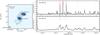 |
Fig. 1 Left: continuum map of I16293 obtained at 220.1 GHz with ALMA. The synthesized beam is shown in the bottom left corner. The rms noise is 3.6 mJy beam-1in the central 20″ region of the map. Contours are drawn to − 3, 3, 10, 22, 39, 61, 88, 120, and 157 time the rms noise, where negative contours are plotted using dotted lines. The peak continuum flux densities for sources A and B are 0.539 ± 0.004 and 1.066 ± 0.004 Jy beam-1, respectively. Right: spectra of sources A and B are shown in the bottom and top panels, respectively. The rms noise in the line-free channels is 4.5 mJy beam-1. The red lines (solid and dotted) show the molecular transitions previously identified by Jørgensen et al. (2011), and the solid lines mark the transition where the inverse P-Cygni profile is found. |
Sources I16293A and I16293B are clearly detected in the continuum map, shown in Fig. 1. The continuum peak fluxes of A and B agree with the fluxes reported previously by Bottinelli et al. (2004) at 230 GHz with a similar beam. The ALMA observations also trace some extended continuum emission connecting sources A and B, which was not detected in the PdBI map of Bottinelli et al. (2004) and is most likely due to spatial filtering and poorer sensitivity of the PdBI observations. This extended continuum emission traces the inner region of the common protostellar envelope as traced by single-dish observations, and includes the position at which Remijan & Hollis (2006) detected an inverse P-Cygni profile in the low-density tracer  (2–1).
The continuum emission is used to estimate the mass as
 where we assumed optically thin emission and a dust opacity per dust mass (κ1.3 mm) of 0.86 cm2 g-1 (thick ice mantles coagulated at 105 cm-3 from Ossenkopf & Henning 1994) and a gas-to-dust ratio of 100. The total flux, measured over the 10-σ region, for sources A and B is 1.30 ± 0.11 and 1.06 ± 0.15 Jy, respectively, which implies a mass of 0.21 and 0.26 M⊙for sources A and B, respectively.
Thanks to the improved sensitivity and spectral resolution offered by ALMA, many (~50) molecular transitions are detected toward the two continuum sources, while previous SMA observations at this frequency only detected six molecular lines toward each object (Jørgensen et al. 2011). The peak spectra toward source A and B are shown in Fig. 1, where we can appreciate the difference in the line profile toward these two objects. A thorough line identification and comparison of chemical properties will be addressed in a future publication.
3.2. Evidence for infalling gas toward source B
Toward I16293B, inverse P-Cygni profiles are unambiguously detected in three molecular lines (see Figs. 2 and C.1). These line profiles are clear evidence for infall in source B. Although an absorption feature in SO (76–66) toward source B was reported by Chandler et al. (2005) as suggestive of infall, the ALMA observations here analyzed are the first observations of the inverse P-Cygni profile toward this source.
The inverse P-Cygni line profiles are modeled to extract the velocity information of the infalling gas and estimate the infall rates. Here we used the simple two-slab model described by Myers et al. (1996) with the modification introduced by Di Francesco et al. (2001) to take into account the continuum source. The model fits the infall velocity of the layers, Vin, its optical depth, τ0, velocity dispersion, σv, and excitation temperature of the layer on the rear, Tr, while the excitation temperature of the foreground layer, Tf, is fixed at 3 K; details of the modeling procedure are described in more detail in Appendix A.
The CH3OCHO-A molecular line with an inverse P-Cygni profile is shown in Fig. 2, with the best two-layer model shown in red (all three molecular lines with an inverse P-Cygni profile are shown in Fig. C.1). The blue excess in the line profiles is not fitted, and therefore the fit is mostly constrained by the absorption feature, see Di Francesco et al. (2001); Kristensen et al. (2012) for similar procedures. Despite its simplicity, the two-layer model contains more parameters than can be fully constrained because of degeneracies in the model, but allows a robust determination of the velocity information. The parameters of the best two-layer model are listed in Table 1.
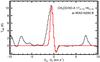 |
Fig. 2 Spectrum toward the continuum peak of I16293B for CH3OCHO-A. The red line shows the best two-layer model of infall fit. The best-fit model parameters are listed in Table 1. See Fig. C.1 for fits of all three molecules. |
Parameters for fitted “two-layer” model.
The infall rate is estimated assuming spherical symmetry as  where at radius rin the infall velocity and density have values of Vin and nin, respectively; and μ is mean molecular weight of the gas (2.3).
The infall radius, rin, can be estimated assuming that the infall velocity is only free-fall,  while also estimating the central mass, M, as that from a uniform density sphere with radius rin and density nin. Therefore, the accretion rate is estimated as
 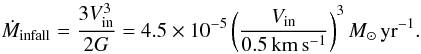 (1)The infall rates obtained using the best fits are 4.2, 4.5, and 4.8 × 10⁻⁵ M⊙ yr-1for CH3OCHO-E, CH3OCHO-A, and H2CCO, respectively.
3.3. Velocity maps
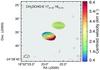 |
Fig. 3 Intensity-weighted velocity for CH3OCHO-E. Contours are drawn to − 3, 3, 10, 22, 39, 61, 88, 120, and 157 times the rms noise of the integrated intensity, 15 mJy beam-1 km s-1, where negative contours are plotted using dotted lines. The beam size is shown at the bottom left corner. See Fig. C.2 for velocity maps of all three molecules. |
The intensity-weighted velocity map for CH3OCHO-E is shown in Fig. 3, where the line-integrated intensity is also overlaid in contours (see Fig. C.2 for maps of all three molecules). The morphology of the emission and its intensity-weighted velocity for CH3OCHO-A and CH3OCHO-E are quite similar, which is not surprising given the almost identical energy level and Einstein coefficients (see Table B.2). For H2CCO, which has a lower energy level than CH3OCHO-A/E, the emission is more extended, but with a similar velocity structure. Source A presents a prominent velocity gradient, with a velocity variation of ~5.5 km s-1across the extent of the molecular emission, which is aligned along the axis connecting the submillimeter sources Aa and Ab previously detected by Chandler et al. (2005). In source B there is no evidence for such a strong velocity gradient, and in fact the velocity variation across the entire source B is ~0.4 km s-1, which is more than an order of magnitude lower than in source A.
The position velocity (PV) diagrams for source A (along the direction shown in Fig. C.2) are consistent with rotation of a disk, which is close to being edge-on (to explain the strong velocity variation). The PV diagrams for the three molecular lines used are shown in Fig. C.3. This orientation would also agree with the orientation of the outflow seen in SiO by Rao et al. (2009). However, the present ALMA data do not rule-out the possibility of two velocity components at scales smaller than our synthesized beam, due for example to the emission of several sources in a multiple system (e.g. Aa, Ab; Chandler et al. 2005).
4. Discussion and conclusion
The molecules where the P-Cygni profile is observed are complex organics, usually associated with the hot-corino and not with the ambient cloud (e.g. Caselli et al. 1993) although some of them have also been detected toward outflows (Arce et al. 2008). Therefore, we can rule out the absorption from the ambient cloud or ambient envelope, and associate the observed P-Cygni profiles to infall from the inner envelope. This infall detection would rule-out the possibility that source B is a young T Tauri star, as previously suggested by Stark et al. (2004). We notice that it is only thanks to the improvement in spectral resolution and sensitivity of the presented ALMA observations compared to previous interferometric observations of this source that the inverse P-Cygni profile could be detected and modeled.
The infall velocity, Vin, derived from the three different molecular lines is the same (0.50 ± 0.01 km s-1) and supersonic. If the velocity dispersion of the absorbing layer is only caused by thermal motions (cs = 0.32 km s-1 for gas at 30 K), the infall velocity is between 1.3 and 1.5 × the sound speed, i.e. supersonic infall. The infall velocity and derived infall rates are consistent with the values derived by Kristensen et al. (2012) for a small sample of low-mass protostars. It is important to note that for source A we could not identify an inverse P-Cygni profile, if present, because of the steep velocity gradient.
The PV diagram for source A is consistent with rotation seen almost edge-on and generated by a central object of 0.53 M⊙, which is consistent with previous estimations using the source kinematics (e.g. Chandler et al. 2005). However, this mass estimate is almost twice as high as the mass estimated using continuum emission (see also Rao et al. 2009). This discrepancy can be reconciled if the dust emission is partially optically thick at submillimeter wavelengths.
The lack of a stronger velocity gradient in source B might be due to either rotation happening at smaller scales than those probed in these observations or because source B is closer to being face-on, which has previously been suggested based on the analysis of the continuum emission (Rodríguez et al. 2005; Loinard et al. 2007).
This work illustrates the new capabilities of ALMA, which open a new window for studying the kinematics and chemistry in the early stages of star-formation. Using ALMA to carry out observations of the kinematics of source A at higher angular resolution will for example allow one to distinguish between the two possible scenarios we propose here to explain the velocity
gradient detected in the present observations, e.g edge-on disk or close binary system.
Online material
Appendix A: The two-layer model
Each inverse P-Cygni profile was fitted using the simple two-slab model described by Myers et al. (1996) with the modification introduced by Di Francesco et al. (2001) to take into account the continuum source, see also Kristensen et al. (2012). The model assumes that the central continuum source is optically thick, emitting as a blackbody of temperature Tc, and filling a fraction of the beam, Φ. Two layers of gas, front and rear, are infalling toward the central source with an infall velocity and velocity dispersion Vin and σv, respectively. The rear layer is illuminated by the background radiation, Tb. If for each layer the peak optical depth is τ0, then the expected line emission at velocity V can be expressed as ![Mathematical equation: \appendix \setcounter{section}{1} \begin{eqnarray} \Delta T_{\rm B}&=& \left(J_{\rm f}-J_{\rm cr}\right) \left[1-{\rm e}^{-\tau_{\rm f}}\right] \nonumber \\&&+\left(1-\Phi\right) (J_{\rm r}-J_{\rm b}) \left[1-{\rm e}^{-(\tau_{\rm r}+\tau_{\rm f})}\right], \end{eqnarray}](/articles/aa/full_html/2012/08/aa19589-12/aa19589-12-eq57.png) (A.1)where
(A.1)where 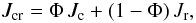 (A.2)and
 ![Mathematical equation: \appendix \setcounter{section}{1} \begin{eqnarray} \tau_{\rm f}&=&\tau_{0}\, \exp{\left[\frac{-(V-(V_{\rm LSR}+V_{\rm in}))^{2}}{2\sigma_{\rm v}^{2}}\right]}\,\\ \tau_{\rm r}&=&\tau_{0}\, \exp{\left[\frac{-(V-(V_{\rm LSR}-V_{\rm in}))^{2}}{2\sigma_{\rm v}^{2}}\right]}, \end{eqnarray}](/articles/aa/full_html/2012/08/aa19589-12/aa19589-12-eq59.png) where VLSR is the source velocity, and the radiation temperature is defined as
where VLSR is the source velocity, and the radiation temperature is defined as ![Mathematical equation: \appendix \setcounter{section}{1} \begin{equation} J_{x}= \frac{T_{0}}{[\exp{(T_{0}/T_{x})}-1]}, \end{equation}](/articles/aa/full_html/2012/08/aa19589-12/aa19589-12-eq61.png) (A.5)where T0 ≡ hν0/kB, and ν0 is the line rest frequency.
(A.5)where T0 ≡ hν0/kB, and ν0 is the line rest frequency.
Since the front absorbing layer is probably subthermally excited, we assumed a conservative value for the excitation front layer of Tf = 3 K. The continuum temperature, Tc, was chosen such that the continuum radiation temperature, Jc(Tc), matches the peak continuum flux in the image. The continuum source beam filling fraction, Φ, which is not well constrained, was set to 0.3 to use the same value as Di Francesco et al. (2001), who modeled interferometric observations with a similar angular resolution as we did; this value is consistent with the line modeling results of coarse angular resolution Herschel data Kristensen et al. (2012). Although the value of Φ used here is arbitrary, we have also performed line profile fits with higher values of Φ and the obtained infall velocity and velocity dispersion are unchanged, while the values for Tr and τ0 are increased and decreased, respectively.Similarly, if a higher value of Tc is used, Tr and τ0 are increased and decreased, respectively, while we obtain the same results for Vin and σv. Therefore our results are robust to the value of Φ and Tc used. An initial set of models with the centroid velocity, VLSR, as a free parameter were run, and all gave a VLSR of 3.4 ± 0.1 km s-1. Given these results, we decided to fix the value of VLSR at 3.4 km s-1and reduce the number of free variables in the fit.
The χ2 was minimized using the mpfitfun procedure (Markwardt 2009), where a spectrum is generated for different parameters and then compared to the observed line profile. The following parameters were kept fixed during the minimization: VLSR, Tc, Tf, and Φ.
Appendix B: Tables
Table B.1 lists the position of the continuum sources. Table B.2 lists the information for the spectral lines analyzed.
Position of sources.
Spectral parameters for lines with inverted P-Cygni profile.
Appendix C: Inverse P-Cygni profiles, centroid velocity and position velocity maps
In this Appendix, we show the inverse P-Cygni profiles and their respective models in Fig. C.1. The centroid velocity maps for all three molecules studied, CH3OCHO-A/E and H2CCO, are shown in Fig. C.2. The position velocity diagrams along the cut shown in Fig. C.2 are shown in Fig. C.3
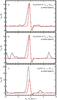 |
Fig. C.1 Molecular line spectra from the ALMA data toward the continuum peak of I16293B. In each panel, a red line shows the best two-layer model of infall fit for each spectrum. The best-fit model parameters are listed in Table 1. |
 |
Fig. C.2 Intensity-weighted velocity for the three lines studied, CH3OCHO-A (left panel) CH3OCHO-E (middle panel), and H2CCO (right panel). Contours are drawn to − 3, 3, 10, 22, 39, 61, 88, 120, and 157 times the rms noise of the integrated intensity, 15 mJy beam-1 km s-1, where negative contours are plotted using dotted lines. The beam size is shown at the bottom left corner. The gray line is the cut used for the position velocity diagram shown in Fig. C.3. |
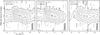 |
Fig. C.3 Position velocity maps of source A, along the direction shown in the rightmost panel of Fig. C.2, for the three lines studied. From left to right: CH3OCHO-A, CH3OCHO-E, and H2CCO. Contours are drawn to − 3, 3, 10, 22, 39, 61, 88, 120, and 157 times the rms noise, 4.5 mJy beam-1, where negative contours are plotted using dotted lines. The red dashed line and red solid circle show the 8 km s-1 arcsec-1velocity gradient and position of source A (VLSR = 3.4 km s-1), respectively. Notice that in all panels an adjacent molecular transition line is marked with a vertical blue line, which can also be identified in Fig. 2. The spatial resolution is shown at the bottom right corner. |
Acknowledgments
This paper makes use of the following ALMA data: ADS/JAO.ALMA#2011.0.00007.SV. ALMA is a partnership of ESO (representing its member states), NSF (USA) and NINS (Japan), together with NRC (Canada) and NSC and ASIAA (Taiwan), in cooperation with the Republic of Chile. The Joint ALMA Observatory is operated by ESO, AUI/NRAO and NAOJ. JEP and AA has received funding from the European Communitys Seventh Framework Programme (/FP7/2007-2013/) under grant agreement No. 229517.
References
- Arce, H. G., Santiago-García, J., Jørgensen, J. K., Tafalla, M., & Bachiller, R. 2008, ApJ, 681, L21 [NASA ADS] [CrossRef] [Google Scholar]
- Bisschop, S. E., Jørgensen, J. K., Bourke, T. L., Bottinelli, S., & van Dishoeck, E. F. 2008, A&A, 488, 959 [NASA ADS] [CrossRef] [EDP Sciences] [Google Scholar]
- Blake, G. A., van Dishoeck, E. F., Jansen, D. J., Groesbeck, T. D., & Mundy, L. G. 1994, ApJ, 428, 680 [NASA ADS] [CrossRef] [Google Scholar]
- Bottinelli, S., Ceccarelli, C., Neri, R., et al. 2004, ApJ, 617, L69 [NASA ADS] [CrossRef] [Google Scholar]
- Caselli, P., Hasegawa, T. I., & Herbst, E. 1993, ApJ, 408, 548 [NASA ADS] [CrossRef] [Google Scholar]
- Castets, A., Ceccarelli, C., Loinard, L., Caux, E., & Lefloch, B. 2001, A&A, 375, 40 [NASA ADS] [CrossRef] [EDP Sciences] [Google Scholar]
- Caux, E., Kahane, C., Castets, A., et al. 2011, A&A, 532, A23 [NASA ADS] [CrossRef] [EDP Sciences] [Google Scholar]
- Cazaux, S., Tielens, A. G. G. M., Ceccarelli, C., et al. 2003, ApJ, 593, L51 [NASA ADS] [CrossRef] [Google Scholar]
- Ceccarelli, C., Castets, A., Loinard, L., Caux, E., & Tielens, A. G. G. M. 1998, A&A, 338, L43 [NASA ADS] [Google Scholar]
- Ceccarelli, C., Loinard, L., Castets, A., Tielens, A. G. G. M., & Caux, E. 2000, A&A, 357, L9 [NASA ADS] [Google Scholar]
- Chandler, C. J., Brogan, C. L., Shirley, Y. L., & Loinard, L. 2005, ApJ, 632, 371 [NASA ADS] [CrossRef] [Google Scholar]
- Correia, J. C., Griffin, M., & Saraceno, P. 2004, A&A, 418, 607 [NASA ADS] [CrossRef] [EDP Sciences] [Google Scholar]
- Coutens, A., Vastel, C., Caux, E., et al. 2012, A&A, 539, A132 [NASA ADS] [CrossRef] [EDP Sciences] [Google Scholar]
- Crimier, N., Ceccarelli, C., Maret, S., et al. 2010, A&A, 519, A65 [NASA ADS] [CrossRef] [EDP Sciences] [Google Scholar]
- Di Francesco, J., Myers, P. C., Wilner, D. J., Ohashi, N., & Mardones, D. 2001, ApJ, 562, 770 [NASA ADS] [CrossRef] [Google Scholar]
- Guarnieri, A., & Huckauf, A. 2003, Z. Naturforsch, 58, 275 [Google Scholar]
- Jørgensen, J. K., Bourke, T. L., Nguyen Luong, Q., & Takakuwa, S. 2011, A&A, 534, A100 [NASA ADS] [CrossRef] [EDP Sciences] [Google Scholar]
- Knude, J., & Hog, E. 1998, A&A, 338, 897 [NASA ADS] [Google Scholar]
- Kristensen, L. E., van Dishoeck, E. F., Bergin, E. A., et al. 2012, A&A, 542, A8 [NASA ADS] [CrossRef] [EDP Sciences] [Google Scholar]
- Kuan, Y.-J., Huang, H.-C., Charnley, S. B., et al. 2004, ApJ, 616, L27 [NASA ADS] [CrossRef] [Google Scholar]
- Loinard, L., Chandler, C. J., Rodríguez, L. F., et al. 2007, ApJ, 670, 1353 [NASA ADS] [CrossRef] [Google Scholar]
- Loinard, L., Torres, R. M., Mioduszewski, A. J., & Rodríguez, L. F. 2008, ApJ, 675, L29 [NASA ADS] [CrossRef] [Google Scholar]
- Looney, L. W., Mundy, L. G., & Welch, W. J. 2000, ApJ, 529, 477 [NASA ADS] [CrossRef] [Google Scholar]
- Maeda, A., De Lucia, F. C., & Herbst, E. 2008, J. Mol. Spectr., 251, 293 [NASA ADS] [CrossRef] [Google Scholar]
- Markwardt, C. B. 2009, in Astronomical Data Analysis Software and Systems XVIII, eds. D. A. Bohlender, D. Durand, & P. Dowler, ASP Conf. Ser., 411, 251 [Google Scholar]
- Mizuno, A., Fukui, Y., Iwata, T., Nozawa, S., & Takano, T. 1990, ApJ, 356, 184 [NASA ADS] [CrossRef] [Google Scholar]
- Müller, H. S. P., Thorwirth, S., Roth, D. A., & Winnewisser, G. 2001, A&A, 370, L49 [NASA ADS] [CrossRef] [EDP Sciences] [Google Scholar]
- Müller, H. S. P., Schlöder, F., Stutzki, J., & Winnewisser, G. 2005, J. Mol. Struct., 742, 215 [NASA ADS] [CrossRef] [Google Scholar]
- Myers, P. C., Mardones, D., Tafalla, M., Williams, J. P., & Wilner, D. J. 1996, ApJ, 465, L133 [NASA ADS] [CrossRef] [Google Scholar]
- Narayanan, G., Walker, C. K., & Buckley, H. D. 1998, ApJ, 496, 292 [NASA ADS] [CrossRef] [Google Scholar]
- Ossenkopf, V., & Henning, T. 1994, A&A, 291, 943 [NASA ADS] [Google Scholar]
- Pickett, H. M., Poynter, R. L., Cohen, E. A., et al. 1998, J. Quant. Spec. Radiat. Transf., 60, 883 [Google Scholar]
- Rao, R., Girart, J. M., Marrone, D. P., Lai, S.-P., & Schnee, S. 2009, ApJ, 707, 921 [NASA ADS] [CrossRef] [Google Scholar]
- Remijan, A. J., & Hollis, J. M. 2006, ApJ, 640, 842 [NASA ADS] [CrossRef] [Google Scholar]
- Rodríguez, L. F., Loinard, L., D’Alessio, P., Wilner, D. J., & Ho, P. T. P. 2005, ApJ, 621, L133 [NASA ADS] [CrossRef] [Google Scholar]
- Schöier, F. L., Jørgensen, J. K., van Dishoeck, E. F., & Blake, G. A. 2002, A&A, 390, 1001 [NASA ADS] [CrossRef] [EDP Sciences] [Google Scholar]
- Stark, R., Sandell, G., Beck, S. C., et al. 2004, ApJ, 608, 341 [NASA ADS] [CrossRef] [Google Scholar]
- Takakuwa, S., Ohashi, N., Bourke, T. L., et al. 2007, ApJ, 662, 431 [NASA ADS] [CrossRef] [Google Scholar]
- van Dishoeck, E. F., Blake, G. A., Jansen, D. J., & Groesbeck, T. D. 1995, ApJ, 447, 760 [NASA ADS] [CrossRef] [Google Scholar]
- Walker, C. K., Lada, C. J., Young, E. T., Maloney, P. R., & Wilking, B. A. 1986, ApJ, 309, L47 [Google Scholar]
- Walker, C. K., Lada, C. J., Young, E. T., & Margulis, M. 1988, ApJ, 332, 335 [NASA ADS] [CrossRef] [Google Scholar]
- Wootten, A. 1989, ApJ, 337, 858 [NASA ADS] [CrossRef] [Google Scholar]
All Tables
All Figures
|
Fig. 1 Left: continuum map of I16293 obtained at 220.1 GHz with ALMA. The synthesized beam is shown in the bottom left corner. The rms noise is 3.6 mJy beam-1in the central 20″ region of the map. Contours are drawn to − 3, 3, 10, 22, 39, 61, 88, 120, and 157 time the rms noise, where negative contours are plotted using dotted lines. The peak continuum flux densities for sources A and B are 0.539 ± 0.004 and 1.066 ± 0.004 Jy beam-1, respectively. Right: spectra of sources A and B are shown in the bottom and top panels, respectively. The rms noise in the line-free channels is 4.5 mJy beam-1. The red lines (solid and dotted) show the molecular transitions previously identified by Jørgensen et al. (2011), and the solid lines mark the transition where the inverse P-Cygni profile is found. |
| In the text | |
|
Fig. 2 Spectrum toward the continuum peak of I16293B for CH3OCHO-A. The red line shows the best two-layer model of infall fit. The best-fit model parameters are listed in Table 1. See Fig. C.1 for fits of all three molecules. |
| In the text | |
|
Fig. 3 Intensity-weighted velocity for CH3OCHO-E. Contours are drawn to − 3, 3, 10, 22, 39, 61, 88, 120, and 157 times the rms noise of the integrated intensity, 15 mJy beam-1 km s-1, where negative contours are plotted using dotted lines. The beam size is shown at the bottom left corner. See Fig. C.2 for velocity maps of all three molecules. |
| In the text | |
|
Fig. C.1 Molecular line spectra from the ALMA data toward the continuum peak of I16293B. In each panel, a red line shows the best two-layer model of infall fit for each spectrum. The best-fit model parameters are listed in Table 1. |
| In the text | |
|
Fig. C.2 Intensity-weighted velocity for the three lines studied, CH3OCHO-A (left panel) CH3OCHO-E (middle panel), and H2CCO (right panel). Contours are drawn to − 3, 3, 10, 22, 39, 61, 88, 120, and 157 times the rms noise of the integrated intensity, 15 mJy beam-1 km s-1, where negative contours are plotted using dotted lines. The beam size is shown at the bottom left corner. The gray line is the cut used for the position velocity diagram shown in Fig. C.3. |
| In the text | |
|
Fig. C.3 Position velocity maps of source A, along the direction shown in the rightmost panel of Fig. C.2, for the three lines studied. From left to right: CH3OCHO-A, CH3OCHO-E, and H2CCO. Contours are drawn to − 3, 3, 10, 22, 39, 61, 88, 120, and 157 times the rms noise, 4.5 mJy beam-1, where negative contours are plotted using dotted lines. The red dashed line and red solid circle show the 8 km s-1 arcsec-1velocity gradient and position of source A (VLSR = 3.4 km s-1), respectively. Notice that in all panels an adjacent molecular transition line is marked with a vertical blue line, which can also be identified in Fig. 2. The spatial resolution is shown at the bottom right corner. |
| In the text | |
Current usage metrics show cumulative count of Article Views (full-text article views including HTML views, PDF and ePub downloads, according to the available data) and Abstracts Views on Vision4Press platform.
Data correspond to usage on the plateform after 2015. The current usage metrics is available 48-96 hours after online publication and is updated daily on week days.
Initial download of the metrics may take a while.