| Issue |
A&A
Volume 544, August 2012
|
|
|---|---|---|
| Article Number | L7 | |
| Number of page(s) | 6 | |
| Section | Letters | |
| DOI | https://doi.org/10.1051/0004-6361/201219589 | |
| Published online | 03 August 2012 | |
Online material
Appendix A: The two-layer model
Each inverse P-Cygni profile was fitted using the simple two-slab model described by Myers et al. (1996) with the modification introduced by Di Francesco et al. (2001) to take into account the continuum source, see also Kristensen et al. (2012). The model assumes that the central continuum source is optically thick, emitting as a blackbody of temperature Tc, and filling a fraction of the beam, Φ. Two layers of gas, front and rear, are infalling toward the central source with an infall velocity and velocity dispersion Vin and σv, respectively. The rear layer is illuminated by the background radiation, Tb. If for each layer the peak optical depth is τ0, then the expected line emission at velocity V can be expressed as 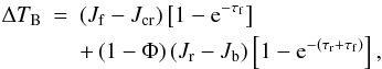 (A.1)where
 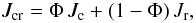 (A.2)and
 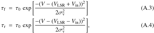 where VLSR is the source velocity, and the radiation temperature is defined as
 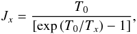 (A.5)where T0 ≡ hν0/kB, and ν0 is the line rest frequency.
Since the front absorbing layer is probably subthermally excited, we assumed a conservative value for the excitation front layer of Tf = 3 K. The continuum temperature, Tc, was chosen such that the continuum radiation temperature, Jc(Tc), matches the peak continuum flux in the image. The continuum source beam filling fraction, Φ, which is not well constrained, was set to 0.3 to use the same value as Di Francesco et al. (2001), who modeled interferometric observations with a similar angular resolution as we did; this value is consistent with the line modeling results of coarse angular resolution Herschel data Kristensen et al. (2012). Although the value of Φ used here is arbitrary, we have also performed line profile fits with higher values of Φ and the obtained infall velocity and velocity dispersion are unchanged, while the values for Tr and τ0 are increased and decreased, respectively.Similarly, if a higher value of Tc is used, Tr and τ0 are increased and decreased, respectively, while we obtain the same results for Vin and σv. Therefore our results are robust to the value of Φ and Tc used. An initial set of models with the centroid velocity, VLSR, as a free parameter were run, and all gave a VLSR of 3.4 ± 0.1 km s-1. Given these results, we decided to fix the value of VLSR at 3.4 km s-1and reduce the number of free variables in the fit.
The χ2 was minimized using the mpfitfun procedure (Markwardt 2009), where a spectrum is generated for different parameters and then compared to the observed line profile. The following parameters were kept fixed during the minimization: VLSR, Tc, Tf, and Φ.
Appendix B: Tables
Table B.1 lists the position of the continuum sources. Table B.2 lists the information for the spectral lines analyzed.
Position of sources.
Spectral parameters for lines with inverted P-Cygni profile.
Appendix C: Inverse P-Cygni profiles, centroid velocity and position velocity maps
In this Appendix, we show the inverse P-Cygni profiles and their respective models in Fig. C.1. The centroid velocity maps for all three molecules studied, CH3OCHO-A/E and H2CCO, are shown in Fig. C.2. The position velocity diagrams along the cut shown in Fig. C.2 are shown in Fig. C.3
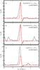 |
Fig. C.1
Molecular line spectra from the ALMA data toward the continuum peak of I16293B. In each panel, a red line shows the best two-layer model of infall fit for each spectrum. The best-fit model parameters are listed in Table 1. |
| Open with DEXTER | |
 |
Fig. C.2
Intensity-weighted velocity for the three lines studied, CH3OCHO-A (left panel) CH3OCHO-E (middle panel), and H2CCO (right panel). Contours are drawn to − 3, 3, 10, 22, 39, 61, 88, 120, and 157 times the rms noise of the integrated intensity, 15 mJy beam-1 km s-1, where negative contours are plotted using dotted lines. The beam size is shown at the bottom left corner. The gray line is the cut used for the position velocity diagram shown in Fig. C.3. |
| Open with DEXTER | |
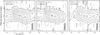 |
Fig. C.3
Position velocity maps of source A, along the direction shown in the rightmost panel of Fig. C.2, for the three lines studied. From left to right: CH3OCHO-A, CH3OCHO-E, and H2CCO. Contours are drawn to − 3, 3, 10, 22, 39, 61, 88, 120, and 157 times the rms noise, 4.5 mJy beam-1, where negative contours are plotted using dotted lines. The red dashed line and red solid circle show the 8 km s-1 arcsec-1velocity gradient and position of source A (VLSR = 3.4 km s-1), respectively. Notice that in all panels an adjacent molecular transition line is marked with a vertical blue line, which can also be identified in Fig. 2. The spatial resolution is shown at the bottom right corner. |
| Open with DEXTER | |
© ESO, 2012
Current usage metrics show cumulative count of Article Views (full-text article views including HTML views, PDF and ePub downloads, according to the available data) and Abstracts Views on Vision4Press platform.
Data correspond to usage on the plateform after 2015. The current usage metrics is available 48-96 hours after online publication and is updated daily on week days.
Initial download of the metrics may take a while.