| Issue |
A&A
Volume 544, August 2012
|
|
|---|---|---|
| Article Number | A55 | |
| Number of page(s) | 9 | |
| Section | Extragalactic astronomy | |
| DOI | https://doi.org/10.1051/0004-6361/201219360 | |
| Published online | 25 July 2012 | |
Spectrally resolved C II emission in M 33 (HerM33es)
Physical conditions and kinematics around BCLMP 691⋆
1
Univ. Bordeaux, Laboratoire d’Astrophysique de Bordeaux,
33270
Floirac,
France
e-mail: This email address is being protected from spambots. You need JavaScript enabled to view it.
2
CNRS, LAB, UMR 5804, 33270
Floirac,
France
3
IRAM, 300 rue de la Piscine, 38406
St Martin d’Hères,
France
4
Instituto Radioastronomia Milimetrica (IRAM),
Av. Divina Pastora 7, Nucleo
Central, 18012
Granada,
Spain
5
Leiden Observatory, Leiden University,
PO Box 9513, NL
2300 RA
Leiden, The
Netherlands
6
SRON Netherlands Institute for Space Research,
Landleven 12,
9747 AD
Groningen, The
Netherlands
7
Tata Institute of Fundamental Research,
Homi Bhabha Road,
Mumbai
400005,
India
8
Laboratoire d’Astrophysique de Marseille – LAM, Université
d’Aix-Marseille & CNRS UMR 7326, 38 rue F. Joliot-Curie, 13388
Marseille Cedex 13,
France
9
Max-Planck-Institut für Astronomie, Königstuhl 17, 69117
Heidelberg,
Germany
10
Max-Planck-Institut für Radioastronomie (MPIfR),
Auf dem Hügel 69,
53121
Bonn,
Germany
11
Astron. Dept., King Abdulaziz University,
PO Box 80203,
Jeddah, Saudi
Arabia
Received: 5 April 2012
Accepted: 15 June 2012
Abstract
This work presents high spectral resolution observations of the [C ii] line at 158 μm, one of the major cooling lines of the interstellar medium, taken with the HIFI heterodyne spectrometer on the Herschel satellite. In BCLMP 691, an H ii region far north (3.3 kpc) in the disk of M 33, the [C ii] and CO line profiles show similar velocities within 0.5 km s-1, while the H i line velocities are systematically shifted towards lower rotation velocities by ~5 km s-1. Observed at the same 12′′angular resolution, the [C ii] lines are broader than those of CO by about 50% but narrower than the H i lines. The [C ii] line intensities also follow those of CO much better than those of H i. A weak shoulder on the [C ii] line suggests a marginal detection of the [13C ii] line, insufficient to constrain the [C ii] optical depth. The velocity coincidence of the CO and [C ii] lines and the morphology at optical/UV wavelengths indicate that the emission is coming from a molecular cloud behind the H ii region. The relative strength of [C ii] with respect to the FIR continuum emission is comparable to that observed in the Magellanic Clouds on similar linear scales but the CO emission relative to [C ii] is stronger in M 33. The [C ii] line to far-infrared continuum ratio suggests a photoelectric heating efficiency of 1.1%. The data, together with published models indicate a UV field G0 ~ 100 in units of the solar neighborhood value, a gas density nH~1000 cm-3, and a gas temperature T ~ 200 K. Adopting these values, we estimate the C+ column density to be NC + ≈ 1.3×1017cm-2. The [C ii] emission comes predominantly from the warm neutral region between the H ii region and the cool molecular cloud behind it. From published abundances, the inferred C+ column corresponds to a hydrogen column density of NH~2×1021cm-2. The CO observations suggest thatNH=2NH2~3.2×1021cm-2 and 21 cm measurements, also at 12′′resolution, yield NH i≈1.2×1021cm-2 within the [C ii] velocity range. Thus, some H2 not detected in CO must be present, in agreement with earlier findings based on the SPIRE 250−500 μm emission.
Key words: galaxies: individual: M 33 / Local Group / galaxies: evolution / galaxies: ISM / ISM: clouds / stars: formation
Herschel is an ESA space observatory with science instruments provided by European-led Principal Investigator consortia and with important participation from NASA.
© ESO, 2012
1. Introduction
The [C ii] line at 157.741 μm is the strongest emission line from galaxies, representing close to one per cent of the bolometric luminosity (Crawford et al. 1985; Stacey et al. 1991; Malhotra et al. 2001) and as such is detectable in very distant objects (Loeb 1993; Maiolino et al. 2005). However, the question of the origin of the [C ii] emission from galaxies (Heiles 1994) remains open to this day. Possible sources are the diffuse warm ionized medium, H ii regions, and mostly neutral photo-dissociation regions (PDRs). Because carbon is ionized more easily than hydrogen (11.26 eV rather than 13.6 eV), [C ii] emission can originate in otherwise neutral gas. A series of [C ii] observations in the Local Group galaxy M 33 with the HIFI (Heterodyne Instrument for Far Infrared astronomy) instrument on the Herschel Space Observatory (Pilbratt 2010; de Graauw et al. 2010; Roelfsema et al. 2012) is the essential component of the open time key project HerM33ES (Kramer et al. 2010). A first article (Mookerjea et al. 2011) presented a PACS map of the [C ii] and [O i] emission and a HIFI [C ii] spectrum of the H ii region BCLMP 302. This work is the first of a series presenting extended high spectral resolution observations of the [C ii] line in M 33.
Despite its importance, only a few velocity-resolved observations have been made of the [C ii] line (e.g. Boreiko & Betz 1991). The goal of such observations is not only to obtain line intensities but also velocity emission profiles to enable a comparison of the velocities and velocity widths of the [C ii]-emitting gas with those of the lines due to CO and HI (and Hα in the future). The [C ii] line emission provides information on the heating and cooling processes of the gas and is a rather unique probe of the photon-dominated region (PDR) between the cool CO-emitting molecular gas and the gas ionized by massive stars. This region is likely to be more massive and extended in sub solar-metallicity galaxies and may represent a significant but hitherto unmeasured gas mass. Hyper-fine components of the [13C ii] line bracket the main isotope (Cooksy et al. 1986) and with HIFI we are, in principle, able to separate the lines allowing a direct determination of the optical depth.
Recently, Langer et al. (2010) found a population of diffuse interstellar clouds (AV < 1.3 mag) in the Milky Way which show [C ii] and H i emission, but no detectable CO emission. The observed [C ii] emission is stronger than expected for diffuse atomic clouds. The idea of CO-dark H2 is not new and (a) some is definitely found around CO-bright clouds (e.g. Pak et al. 1998; Wolfire et al. 2010) but possibly also (b) mixed with the H i (e.g. Papadopoulos et al. 2002) or (c) in the outermost parts of galactic disks (e.g. Pfenniger et al. 1994). Langer et al. (2010) attribute the [C ii] excess emission to diffuse and warm (T ≳ 100 K) molecular (H2) clouds. While the linear resolution of these observations is excellent, the Galactic plane is optically thick at short wavelengths such as the Hα line commonly used to trace H ii regions. Thus, some of the [C ii] emission they detect may in fact be due to ionized rather than neutral gas. The observations presented here allow us to address the same questions with ~50 pc resolution but with the advantage of much clearer views of the region and of the sources of emission at all wavelengths.
Previous observations have established that [C ii] emission is a good tracer of star formation regions. Among Local Group galaxies, there is an excellent correspondence between [C ii] and far-IR emission in both Magellanic Clouds (Poglitsch et al. 1995; Israel et al. 1996; Israel & Maloney 2011) and between [C ii] and both Hα and mid-IR (24 μm) emission in the spiral arms of M 31 (Rodríguez-Fernández et al. 2006). The fact that the [C ii] line represents a similar fraction of the global FIR luminosity of spiral galaxies shows that this also holds in a statistical way on galactic scales.
As illustrated in Fig. 1, the HerM33es project observes [C ii] in a long strip along the major axis. In this work, we investigate the relationship between [C ii] FIR, CO, and H i emission at the scale of individual clouds (~50 pc) in an area centered on the H ii region BCLMP 691 (Boulesteix et al. 1974) and compare it with the results from Mookerjea et al. (2011) on BCLMP 302, both part of the strip. In particular, we estimate the amount of gas traced by the [C ii] emission and and relate that to the CO and HI emission.
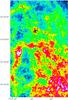 |
Fig. 1 North-eastern part of M 33 in the IRAC 8 μm band (Verley et al. 2007). The upper (small) rectangle shows the region presented in Fig. 2 and the small triangles forming an “X” in and around the rectangle indicate the individual positions of the [C ii] HIFI observations. The large lower rectangle shows the region around BCLMP302 observed with PACS by Mookerjea et al. (2011). The center of M 33 is at the position of the triangle to the lower right of the image of M 33. The giant H ii region NGC 604 can be seen as the very bright region to the left around Dec 30:47 and is marked with a × . |
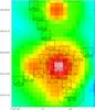 |
Fig. 2 [C ii] spectra superposed on a Spitzer 24 μm image at 6′′ resolution of BCLMP 691. The dotted blue contours show the Hα emission at levels of 100, 300, 1000, 3000, and 10 000 counts (Greenawalt 1998; Hoopes & Walterbos 2000). Only positions with detected [C ii] flux are shown. The velocity scale is from −300 to −230 km s-1 and the y axis is from −0.2 K to 1 K. The beamsize is shown as a circle around the southernmost spectrum. |
2. Observations and data reduction
The HIFI Wide Band Spectrometer horizontal and vertical polarization data were processed to level 2 using the standard pipeline of HIPE version 4 and then exported to CLASS1. The obsids for the BCLMP691 observations are 1342213155 and 1342213156 which are load-chop on-the-fly maps consisting of 8280 individual spectra each. The maps are perpendicular strips with position angles of 22.5 and 112.5 degrees with close spacing between individual spectra. All spectra were smoothed to 8 MHz (1.26 km s-1) resolution and a zero-order baseline (i.e. a continuum level) was subtracted excluding velocities from −280−255 km s-1, corresponding to the expected line velocity. The baseline was calculated over a region extending from −345 to −170 km s-1. All velocities are in the LSR frame and the systemic velocity of M 33 is about −170 km s-1.
A number of spectra (roughly 1/3) suffer from the HIFI hot electron bolometer (HEB) standing wave pattern at about 290 MHz. Various Fourier filtering schemes were applied but it proved very difficult to reliably eliminate the standing waves. In the end, the 11 298 good spectra were kept and the others dropped.
At 5′′ intervals along the cross, the spectra were convolved with a 5′′ Gaussian in order to obtain a single high quality spectrum at each position. The resulting beam size is 12.3 × 11.4′′ because the convolution only stretches the beam in the direction where there are spectra (i.e. along the lines of the cross). In the center, the beam is more circular because both arms of the cross are included in the convolution. Four “extra” spectra were generated near the center at (± 5′′, ± 5′′) with respect to the cross (see Fig. 2). Although no pointings correspond exactly to these positions, this is possible because the neighboring beams overlap considerably in this region so these points are sampled on both arms of the cross.
Positions observed in [C ii].
Velocities, line widths, and line intensities were measured from Gaussian fits to the 17 detected positions on the cross plus the 4 “extra” positions. Table 1 gives the positions of the spectra with the fit results for the detected positions and the rms noise level for the others. The uncertainties come from the Gaussian fits using the CLASS fitting routine. As per the current HIFI users manual2, we adopt a main beam efficiency of 0.693 and present all data on the main beam temperature scale.
3. Analysis of BCLMP 691 [C II] line intensities
3.1. The H II region complex BCLMP 691
Both BCLMP 691 (IK 60, Aller 3, Searle 15) and BCLMP 302 (als known as IK 53, Aller 43, Searle 11) are among the brighter nebulae in the northern half of M 33 with 1.4 GHz flux densities of 4.6 and 6.1 mJy respectively (Boulesteix et al. 1974; Israel & van der Kruit 1974). Figure 1 shows the northern part of M 33 with the region observed around BCLMP 691 (and BCLMP 302) indicated. Zooming in on BCLMP 691, Figure 2 shows the [C ii] detections superposed on a 24 μm image (Tabatabaei et al. 2007) of the region. BCLMP 691 and BCLMP 302 are similar in many aspects. Both are about 75 pc in diameter with large-scale rms electron densities of  of 7.4 and 6.3 cm-3 and excitation parameters of
  and 200 pc cm-2, corresponding to excitation by the equivalent of 3 and 4 O5 exciting stars (Israel & van der Kruit 1974). More significant differences between BCLMP 691, the H ii region studied in this paper, and BCLMP 302 (Mookerjea et al. 2011) are tied to their location. BCLMP 691 is a major H ii region 3.3 kpc from the center, and relatively isolated, whereas BCLMP 302 is a major star-forming region embedded in the northern spiral arm at 2.1 kpc from the center of M 33. The H i and CO(J = 2−1) emission towards the latter is stronger than towards BCLMP 691. BCLMP 691 has a metallicity 12 + log (O/H) = 8.42 ± 0.06 (Magrini et al. 2010), i.e. an oxygen abundance relative to H of 2.6 × 10⁻⁴, about half the metallicity of the solar neighborhood. This is somewhat below the average of the more central H ii regions such as NGC 595 (Magrini et al. 2010). BCLMP 302 is irradiated by the combined young and old stellar population of the northern spiral arm, but in the vicinity of BCLMP 691, the radiation field from the old stellar population is weak. Nevertheless, the difference in ionization between the two regions is remarkable: the isolated complex BCLMP 691 has a much higher degree of ionization than BCLMP 302, with ratios Ne++/Ne+ = 1.25 (0.19) and S3+/S++ = 0.15 (0.04) where the values in parentheses are those of BCLMP 302 (Rubin et al. 2008). The ionization difference may be attributable to the lower metallicities at greater radii causing the exciting stars to have harder radiation fields. As can be seen in the Appendix of Gratier et al. (2012), the geometry of the H ii region – molecular cloud interface differs between BCLMP 302 and 691 (clouds 256 and 299 of Gratier et al. 2012). It is clearly of interest to identify the corresponding effects on the [C ii] emission.
3.2. The [C II] to FIR and the [C II] to CO ratios
The large-scale [C ii] to FIR continuum flux ratio in normal galaxies is usually below 1%, typically 0.3−0.5% (Crawford et al. 1985; Stacey et al. 1991; Braine & Hughes 1999; Malhotra et al. 2001). Here, FIR refers to the dust emission in the wavelength range 42−122μm (IRAS definition). This is about half of all dust emission (i.e. FIR ≈ 1/2 TIR, see Dale & Helou 2002). At the scale of a spiral arm in M 31, using ISO LWS data at 300 pc resolution, Rodríguez-Fernández et al. (2006) find a considerably higher ratio (I[C ii]/FIR42−122 ≈ 2%). The closest to M 33 in metallicity is the LMC, where Israel et al. (1996) and Israel & Maloney (2011) find ICII/FIR flux ratios between of 0.7 and 5.0%. The [C ii] flux can be calculated as  (1)where ∫Tdv is the integrated intensity in the standard units of K km s-1 (the 105 converts from K km s-1 to K cm s-1).
For BCLMP 691 we find a ratio of I[C ii]/FIR42−122 ≈ 1.1% and a ratio of [C ii] flux to total dust emission of 0.54%. The I[C ii]/IR ratio is indicative of the gas heating efficiency (Bakes & Tielens 1994) and the value for BCLMP 691 is very close to the average ratio obtained by Mookerjea et al. (2011) for BCLMP 302 (their region A). In this discussion we focus on the center of the H ii region, our (0, 0) position. The FIR and total dust luminosities for this region were calculated by directly summing the emission in these wavebands using the 5.8, 24, and 70 μm emission from Spitzer and the PACS and SPIRE data obtained by the HerM33es project. PAH emission has been left out of the total dust flux. In both M 33 fields observed, these ratios are thus very similar to each other and to those obtained in the LMC and the SMC (Israel & Maloney 2011).
We may also compare the [C ii] to CO flux ratios for the various environments. Unfortunately, we do not have J = 1−0 12CO measurements at 12′′ resolution so we have convolved our CO(2−1) observations to the 25′′ resolution of the CO(1−0). At this 100 pc resolution, the CO(2−1)/(1−0) line ratio is 0.72, very close to the average value given in Gratier et al. (2010).
For BCLMP 691, a comparison of [C ii] and CO lines can be found in Table 1 and the spectra are superposed in Fig. 3. As for [C ii], the CO flux can be calculated as  × 10-9∫TCO(1−0)dv where ∫Tdv is in K km s-1 as usual. Assuming the CO(2−1)/(1−0) line ratio is also 0.72 at 12′′ resolution, we find a I[C ii]/ICO(1−0) flux ratio of about 8000 for BCLMP 691, slightly lower than the BCLMP 302 peak value (Mookerjea et al. 2011). Although this is in excess of the ratios of about 1500 found in normal spiral galaxies, and even of ratios of 6000 such as found in starburst galaxies (Stacey et al. 1991; Braine & Hughes 1999), it is considerably lower than the corresponding ratios found in the LMC, which (with one exception, N 159W) range from 13 000 to more than 100 000 with a mean of 60 000 for the individual star-forming clouds observed, and a ratio of 23 000 for the LMC as a whole (Israel et al. 1996; Israel & Maloney 2011).
In general, because of its (indirect) dependence on UV photons, [C ii] emission is linked to star formation. GMCs without H ii regions have much weaker [C ii] emission for comparable levels of CO emission, such as N 159S in the LMC with a I[C ii]/ICO ratio of 400 (Israel et al. 1996). In comparison with the LMC clouds, the two objects in M 33 have rather low I[C ii]/ICO ratios although I[C ii]/FIR ratios are practically identical. Since the latter are a measure of the heating efficiency of the clouds, the conclusion must be that otherwise comparable star-forming complexes are much richer in CO in M 33 than in the LMC. Since there is no difference in this respect between the two M 33 objects, the degree of ionization, i.e. the hardness of the radiation field, is not a factor of significance.
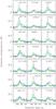 |
Fig. 3 [C ii], CO, and H i spectra of all detected positions at 12′′ resolution. Offsets in arcsec are indicated in the upper right corner of each panel. The order follows that of Table 1from bottom left to upper right. [C ii] is in black, CO in green, and H i is in blue. Y-scale is main beam antenna temperature in Kelvins for [C ii] and CO; H i temperatures need to be multiplied by 150 to obtain true antenna temperatures. |
3.3. Carbon column density
3.3.1. A lower limit to NC+
The [C ii] line is an important probe of the physical conditions of the ISM. In particular, it provides information on regions not probed by the CO line and possibly not probed by the H i line. The [C ii] line is thermalized at a density of about 3000 cm-3 in neutral gas and has an upper level energy of 91 K. Thus, a minimum [C ii] column density can be calculated assuming that densities ≫ 3000 cm-3 and temperatures ≫ 91 K. Lower densities and/or lower temperatures would decrease the [C ii] emission per H-atom. A lower limit to the hydrogen column density can be determined by assuming a carbon abundance. Israel et al. (1996) and Israel & Maloney (2011) performed comparable studies at very similar linear resolutions in the brightest H ii region complexes of the Large Magellanic Cloud, which has a metallicity similar to that of M 33. These studies therefore provide an excellent basis for comparison, even though they did not measure the actual [C ii] line profiles. Following the reasoning and equations presented by Crawford et al. (1985) and Israel et al. (1996), 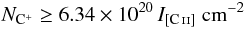 (2)with I [C ii] defined in Eq. (1).
The [C ii] line intensity at the peak of 9.9 K km s-1 is equivalent to 7.0 × 10⁻⁵ erg cm-2 s-1 sr-1, or a column density of NC + ≥ 4.4 × 1016 cm-2. We emphasize once more that this is a lower limit because of the high-density, high-temperature assumption underlying these numbers. We have also assumed that all of the ionized carbon was singly ionized – this latter hypothesis is reasonable for the neutral medium (i.e. where H is not ionized).
That carbon is only singly ionized is not a good approximation for regions where H ii is the dominant phase. The ionization potential for doubly-ionized carbon is 24.38 eV, considerably below that of doubly-ionized neon (40.96 eV) or triply ionized sulphur (34.83 eV). Given the high degree of ionization characterizing BCLMP 691 (Sect. 3.1), in the H ii region itself most carbon will be in the higher ionization states. Therefore, in the following, we will compare the derived carbon column density with that of the neutral gas. By the same token, we expect little of the [C ii] emission to be contributed by the ionized gas in the H ii region, which would have caused us to overestimate the amount of emission from the neutral gas. Rather, we may assume that essentially all of the [C ii] is indeed associated with the H i and H2. As Mookerjea et al. (2011) have estimated that emission from the H ii region BCLMP 302 might account for 20−30% of the [C ii] emission, this is another potential distinction between that complex and the one studied here.
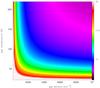 |
Fig. 4 Log of the C+ column density as a function of gas density and temperature for the [C ii] intensity at the (0, 0) position of I [C ii] = 7.0 × 10⁻⁵ erg cm-2 s-1 sr-1. The bottom of the color scale (black) shows the high-temperature high density limit from Eq. (2) which yields log(NC + ) ≥ 16.65 – in the range of parameter space presented here, the limit is not reached. The column densities are for optically thin emission. Contours are plotted at column densities of log(NC+) = 17, 17.3, and 17.6. We have used Eq. (A1) from Crawford et al. (1985) assuming a critical density of 3000 cm-3. |
3.3.2. A more realistic estimate of NC+
We can get an idea of how much of an underestimate Eq. (2) is by looking at Fig. 4, which shows ionized carbon column density variations as a function of density and temperature for low optical depths. Under these conditions the C+ column density is proportional to the [C ii] line intensity, so that we can use this diagnostic diagram to calculate C+ column densities when information about the temperature and density of the gas is available. Throughout, the ratio between NC + and I [C ii] is at least twice that of Eq. (2), except in the very high temperature, very high density regime (the violet region at the upper right).
It is unlikely that the gas (or the dust) in BCLMP 691 has a temperature T ≫ 91 K and density n ≫ 3000 cm-3 on the (linear) scales we are sensitive to here. As noted before, these scales are almost identical to those Israel et al. (1996) and Israel & Maloney (2011) were sensitive to in the LMC. In the LMC regions N 159, N 160, and N 11 they estimate G0 to vary between 25 and 450. Assuming the flux impinging on a dust cloud is Istar = 4πIdust, where the 4π converts the erg cm-2 s-1 sr-1 to erg cm-2 s-1, that half of the stellar flux Istar is due to photons with hν < 6 eV (e.g. Tielens & Hollenbach 1985), we can estimate the FUV (6 < hν < 13.6 eV) flux expressed in units of the Habing (1968) field to be G0 = 2πIdust/1.6 × 10-3.
Direct integration of the dust emission from 5 to 610 μm (the edge of the SPIRE 500 μm band) yields a peak flux of 0.013 erg cm-2 s-1 sr-1, corresponding to G0 = 51, well within the range found to apply to the LMC clouds. Since the core of the H ii region BCLMP 691 is smaller than the 12′′ beam (see Hα contours in Fig. 2), the central G0 is likely to be somewhat higher but probably lower than in N159 or N160. At these temperatures, the dust should emit strongly in the Spitzer 24 and 70 μm bands; if the grains are in thermal equilibrium, then a temperature of about 90 K is suggested by the flux ratio and the gas kinetic temperature should be somewhat higher (Hollenbach & Tielens 1999). The strong 5.8 μm emission shows that some warmer dust is also present. In N159 and N160, Israel et al. (1996) estimate that the C+ column density is 2−4 times higher than the limit given by Eq. (2). As G0 rises, we expect the gas temperature to rise, moving C+ column densities towards the limit expressed by Eq. (2). Hence, for BCLMP 691, our best estimate is a column density NC + ≈ 1.3 ± 0.4 × 1017 cm-2, 3 times the lower limit in Eq. (2). Below, we confirm this estimate using the Kaufman et al. (1999) PDR model.
3.3.3. Hydrogen column density NH
There are no direct measurements of the carbon abundance in BCLMP 691. However, Esteban et al. (2009) estimate carbon and oxygen abundances for NGC 595 and NGC 604 and the C/O ratios they find are [C]/[O] = −0.16 and −0.20. They present models by Carigi et al. (2005) that suggest C/O ratios of about [C]/[O] = −0.33. Based on the models and these recent and high-quality data, we assume [C]/[O] = −0.25 ± 0.08 yielding a carbon abundance for BCLMP 691 of 12 + log [C]/[H] = 8.17 ± 0.1, or a C abundance of 1.48 × 10⁻⁴ ± 25% after propagating the (independent) uncertainties given above for the O abundance and the C/O ratio. If we assume that half of the carbon is locked in dust grains, this leads us to a gas-phase C abundance of 7.4 × 10⁻⁵. Therefore, for NC + ≈ 1.3 × 1017 cm-2, the H column density is about NH ≈ 1.8 × 1021 cm-2. If the fraction of carbon locked in dust is 2/3 (as suggested by Table 2 of Sofia et al. 2011), then the gas-phase C abundance would be correspondingly lower and the H column density would become NH ≈ 2.6 × 1021 cm-2.
 |
Fig. 5 [C ii] spectrum of the sum of the 5 strongest positions of the cross and a Gaussian fit (green), showing the shoulder at v ≈ −259 km s-1 and the velocity where [13C ii] emission would be expected. The average CO spectrum of these positions is shown as a dashed line. The lower panel shows the [C ii] residual (spectrum minus Gaussian fit). |
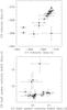 |
Fig. 6 (Top) Comparison of CO and [C ii] velocities, showing the good agreement. (Bottom) Comparison of CO and [C ii] line widths, showing that with the exception of some positions with large uncertainties, the CO lines are narrower. The velocities, line widths, and their uncertainties, have been measured by Gaussian fits to the spectra. |
We can compare this column density with that of the H i and the CO. The H i column density at 12′′ resolution towards the center of BCLMP 691 is NH i = 1.7 × 1021 cm-2, of which 1.2 × 1021 cm-2 is within the [C ii] velocity range. Assuming a conversion factor N(H2)/ICO = 4 × 1020 cm-2/(K km s-1), twice that of the Galactic disk, the molecular gas column density is NH = 2N(H2) ≈ 3.2 × 1021 cm-2. The [C i] line has not been observed in BCLMP 691. At larger scales, the whole H ii region emits about 2% of the Hα flux of M 33 and the associated molecular cloud 299, which is about the same size as the H ii region (see table in Gratier et al. 2012), emits about 0.1% of the CO emission.
4. Analysis of BCLMP 691 [C II] line profiles
4.1. The 13C II line
The three hyperfine components of the [13C ii] line have frequencies equivalent to offsets of −66, + 11, and + 63 km s-1, respectively, from the [12C ii] line center at 1 900 536.9 ± 1.3 MHz (Cooksy et al. 1986; Stacey et al. 1991; Boreiko & Betz 1996). The ratio of the sum of the three hyperfine [13C ii] transitions to the [12C ii] line intensity, coupled with the relative abundance ratio, provides a measure of the optical depth of the [12C ii] emission (e.g. Stacey et al. 1991). We have searched for a possible signature of [13C ii] emission in the inner regions of BLMP 691 where the + 11 km s-1 component may occur as a shoulder present on the [12C ii] line. After fitting a Gaussian to the sum of the five strongest detections (the 0, 0 spectrum and the first spectrum on each leg of the cross), we find that the Gaussian fit is good on the blue side (− 280 km s-1) but leaves an excess on the red side, at 10−11 km s-1 from the [C ii] line center (see Fig. 5). This transition, F = 2 → 1, is expected to be the strongest of the three hyperfine transitions (Cooksy et al. 1986). Although the velocity coverage of the spectra includes the two other components, they are not detected. The lower panel of Fig. 5 shows the residual (spectrum minus Gaussian fit) with the nominal position of the [13C ii] line. Using 10 km s-1 windows shifted by −66, + 11, and + 63 km s-1 with respect to the [12C ii] line center, we find a nominal summed [13C ii] line intensity of 0.31 ± 0.23 K km s-1, i.e. a ratio 97 > I12/13 > 16 with one sigma uncertainties.
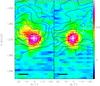 |
Fig. 7 Position-velocity plots along the two arms of the observed HIFI cross. Left: perpendicular to the major axis of the galaxy, right: along the major axis of the galaxy. For each plot the color bitmap is the [C ii] in main beam temperature (Kelvins), the white contours are the CO(2−1) Tmb temperature every 0.1 K starting from 0.1 K, the dark blue contours are the H i temperature every 10 K starting from 10 K. The horizontal bar at the bottom of each panel indicates the 12′′ beamsize of the observations. |
4.2. [C II] line profiles compared to CO and H I
As can be seen from both Table 1 and Fig. 6, the CO and [C ii] radial velocities determined from Gaussian fits agree very well, generally to within half of a CO velocity channel. The exception is the relatively poor measurement at position (+7.7, +18.5) which is a (3.5σ) detection with a very large uncertainty associated with both the velocity and line width. In BCLMP 302, Mookerjea et al. (2011) find a mean velocity difference between CO and [C ii] of 1.3 km s-1, presumably reflecting physical motion (outflow?) of one of the gaseous components giving rise to the [C ii] emission. We do not find such a velocity difference in BCLMP 691 but that could well be a question of geometry. The [C ii] profiles presented here are similar in width to the HIFI spectrum presented by Mookerjea et al., as are the CO profiles.
The [C ii], H i, and CO spectra for all positions detected in [C ii] are presented in Fig. 3. While H i is detected everywhere, the CO emission peaks in the regions where [C ii] was detected. The CO and [C ii] profiles are similar in shape although the [C ii] lines are broader. H i, on the other hand, is systematically shifted to more positive radial velocities (i.e. lower rotation velocities) by about 5 km s-1 and the CO and [C ii] profiles are at the high rotation velocity edge of the H i. Only a few of the [C ii] spectra show emission at velocities similar to those of the H i (e.g. low rotation velocity tail of emission at offsets 9.2, −3.8 and 13.9, −5.7).
Figure 7 presents a comparison of the position-velocity (PV) plots of [C ii], CO, and H i along the two arms of the cross observed in [C ii]. In both directions, the CO temperature and CO velocity follow those of [C ii] closely but the H i profiles seem uncorrelated in temperature and spread over a much broader range in velocities (typically ~20 km s-1). Figure 6 shows the general agreement in velocities between CO and [C ii] in a different way but it also suggests (lower panel) that the line widths mostly fall into two groups. The brighter regions (smaller error bars) define a distribution where the CO line width is essentially constant while the [C ii] line width varies by a factor two. At the very least this indicates that the CO-emitting gas is dynamically cooler, less affected by the processes that cause large-scale motions in the bright [C ii] emitting region. The weaker regions, on the other hand, show a pattern where both CO and [C ii] appear to vary linearly with each other. These regions correspond to the more diffuse ISM. Looking more closely at the bright regions (i.e. ignoring the regions with larger error bars) we see that there may be a division into two further groups with [C ii] widths of ~10 km s-1 and ~15 km s-1 respectively and CO widths of ~7 km s-1 and ~8 km s-1 respectively. The broad and strong [C ii] lines are found along the Hα-bright extension to the SE.
5. Synthesis and conclusions
In order to better locate BCLMP 691 on the diagnostic diagram in Fig. 4, we need an estimate of the temperature, density, or a combination. We can place the [C ii]/FIR ratio of ~0.011 derived in Sect. 3.2 in Fig. 11 in Bakes & Tielens (1994) and find that the product  . For a neutral region, the electrons will come from the singly ionized carbon so ne ≈ nH 7.4 × 10⁻⁵ (see Sect. 3.3.3). Noting G2 = G0/100, T = 100T2, and nH = 1000n3, we obtain
  . In Sect. 3.1.2 we estimated G0 ~ 50 but pointed out that this could be an underestimate by a factor 2. Kaufman et al. (1999) estimate gas temperatures varying from 300 K to 100 K for G0 = 100 as densities climb from 100 to 10 000 cm-3, with nH = 1000 corresponding to T ≈ 200 K.
The general similarity between BCLMP 691 and BCLMP 302 holds also for the [C ii]/[O i] ratio, which is [C ii]/[O i] ≳ 1 in both regions (see Table 7 in Mookerjea et al. 2011; and Nikola et al., in prep.). Looking at e.g. Fig. 4 of Kaufman et al. (1999), we see that for a constant [C ii]/[O i] ratio, nH decreases when T increases. The “solution” G0 ~ 100, nH ~ 1000 seems to be a good fit and the value of T ~ 200 K fits both with the Kaufman et al. (1999) PDR model and with the [C ii]/FIR ratio via the calculations in Bakes & Tielens (1994). Looking back at Fig. 4, the [C ii] column density is about N [C ii] ~ 1.3 × 1017 cm-2, in good agreement with Sect. 3.3.2. It may be worth noting that some “extra” H2 was found by Braine et al. (2010) through correlating the Herschel/SPIRE cool dust measurements with CO and H i observations. Their interpretation was indeed that this column density could likely be attributed to regions, cloud envelopes, where the CO was photo-dissociated but the gas remained predominantly molecular. The 1.3 ± × 1017 cm-2 C+ column we observe comes from this layer of H i and H2 exterior to the region where most carbon is in CO. As the C+ layer contains more H than is observed in H i, particularly when considering only the H i within the velocity range detected in [C ii], some molecular gas not detected via CO must be present.
The correspondence along the cross between the [C ii] and CO intensities and velocities is quite good (see e.g. Fig. 3) in BCLMP 691 but this is not the case for all regions. We suspect that this may be a question of geometry and that in BCLMP 691 we are probably seeing the H ii region with the molecular cloud right behind it such that the surface of the cloud is in the same direction as the bulk of the cloud (where carbon is in CO). At the scale of this H ii region, the [C ii] emission is clearly coming from the PDR, plus perhaps the ionized skin. BCLMP 691 appears to be part of molecular cloud 299 in the Gratier et al. (2012) catalog. The strong emission in all wavebands tracing star formation, including the FUV, suggests that indeed the H ii region is on the near side of the GMC. While we use the term “cloud”, molecular clouds have substructure so the exposed material may have a rather intricate perimeter. The CO peak is actually just south-east of the Hα peak (the H ii region) but the FUV, 8, and 24 μm emission all peak on the H ii region, implying that the warm part of the molecular cloud is behind the H ii region. Since the [C ii] emission is coming from the near side of the molecular cloud, it is not surprising that it shares the same dynamics (velocities, Fig. 6). Perhaps due to the geometry, these observations of BCLMP 691 show clearly that the [C ii] emission is coming from the molecular cloud – H ii region
interface, as in models of photo-dissociation regions (Tielens & Hollenbach 1985; Kaufman et al. 1999).
Acknowledgments
The authors would like to thank Laura Magrini for useful discussions on abundances in M 33. HIFI has been designed and built by a consortium of institutes and university departments from across Europe, Canada, and the United States under the leadership of SRON Netherlands Institute for Space Research, Groningen, The Netherlands, and with major contributions from Germany, France, and the US. Consortium members are: Canada: CSA, U. Waterloo; France: CESR, LAB, LERMA, IRAM; Germany: KOSMA, MPIfR, MPS; Ireland: NUI Maynooth; Italy: ASI, IFSI-INAF, Osservatorio Astrofisico di Arcetri-INAF; Netherlands: SRON, TUD; Poland: CAMK, CBK; Spain: Observatorio Astronómico Nacional (IGN), Centro de Astrobiología (CSIC-INTA); Sweden: Chalmers University of Technology MC2, RSS & GARD; Onsala Space Observatory; Swedish National Space Board, Stockholm University Stockholm Observatory; Switzerland: ETH Zurich, FHNW; USA: Caltech, JPL, NHSC. HIPE is a joint development by the Herschel Science Ground Segment Consortium, consisting of ESA, the NASA Herschel Science Center, and the HIFI, PACS and SPIRE consortia. We also thank the French Space Agency CNES for financial support.
References
- Bakes, E. L. O., & Tielens, A. G. G. M. 1994, ApJ, 427, 822 [NASA ADS] [CrossRef] [Google Scholar]
- Boreiko, R. T., & Betz, A. L. 1991, ApJ, 380, L27 [NASA ADS] [CrossRef] [Google Scholar]
- Boreiko, R. T., & Betz, A. L. 1996, ApJ, 467, L113 [NASA ADS] [CrossRef] [Google Scholar]
- Boulesteix, J., Courtes, G., Laval, A., Monnet, G., & Petit, H. 1974, A&A, 37, 33 [NASA ADS] [Google Scholar]
- Braine, J., & Hughes, D. H. 1999, A&A, 344, 779 [NASA ADS] [Google Scholar]
- Braine, J., Gratier, P., Kramer, C., et al. 2010, A&A, 520, A107 [NASA ADS] [CrossRef] [EDP Sciences] [Google Scholar]
- Carigi, L., Peimbert, M., Esteban, C., & García-Rojas, J. 2005, ApJ, 623, 213 [NASA ADS] [CrossRef] [Google Scholar]
- Cooksy, A. L., Blake, G. A., & Saykally, R. J. 1986, ApJ, 305, L89 [NASA ADS] [CrossRef] [Google Scholar]
- Crawford, M. K., Genzel, R., Townes, C. H., & Watson, D. M. 1985, ApJ, 291, 755 [NASA ADS] [CrossRef] [Google Scholar]
- Dale, D. A., & Helou, G. 2002, ApJ, 576, 159 [NASA ADS] [CrossRef] [Google Scholar]
- de Graauw, T., Helmich, F. P., Phillips, T. G., et al. 2010, A&A, 518, L6 [NASA ADS] [CrossRef] [EDP Sciences] [Google Scholar]
- Esteban, C., Bresolin, F., Peimbert, M., et al. 2009, ApJ, 700, 654 [NASA ADS] [CrossRef] [Google Scholar]
- Gratier, P., Braine, J., Rodriguez-Fernandez, N. J., et al. 2010, A&A, 522, A3 [NASA ADS] [CrossRef] [EDP Sciences] [Google Scholar]
- Gratier, P., Braine, J., Rodriguez-Fernandez, N. J., et al. 2012, A&A, 542, 108 [Google Scholar]
- Greenawalt, B. E. 1998, Ph.D. Thesis, New Mexico State University [Google Scholar]
- Habing, H. J. 1968, Bull. Astron. Inst. Netherlands, 19, 421 [Google Scholar]
- Heiles, C. 1994, ApJ, 436, 720 [NASA ADS] [CrossRef] [Google Scholar]
- Hollenbach, D. J., & Tielens, A. G. G. M. 1999, Rev. Mod. Phys., 71, 173 [Google Scholar]
- Hoopes, C. G., & Walterbos, R. A. M. 2000, ApJ, 541, 597 [NASA ADS] [CrossRef] [Google Scholar]
- Israel, F. P., & Maloney, P. R. 2011, A&A, 531, A19 [NASA ADS] [CrossRef] [EDP Sciences] [Google Scholar]
- Israel, F. P., & van der Kruit, P. C. 1974, A&A, 32, 363 [NASA ADS] [Google Scholar]
- Israel, F. P., Maloney, P. R., Geis, N., et al. 1996, ApJ, 465, 738 [NASA ADS] [CrossRef] [Google Scholar]
- Kaufman, M. J., Wolfire, M. G., Hollenbach, D. J., & Luhman, M. L. 1999, ApJ, 527, 795 [NASA ADS] [CrossRef] [Google Scholar]
- Kramer, C., Buchbender, C., Xilouris, E. M., et al. 2010, A&A, 518, L67 [NASA ADS] [CrossRef] [EDP Sciences] [Google Scholar]
- Langer, W. D., Velusamy, T., Pineda, J. L., et al. 2010, A&A, 521, L17 [Google Scholar]
- Loeb, A. 1993, ApJ, 404, L37 [NASA ADS] [CrossRef] [Google Scholar]
- Magrini, L., Stanghellini, L., Corbelli, E., Galli, D., & Villaver, E. 2010, A&A, 512, A63 [NASA ADS] [CrossRef] [EDP Sciences] [Google Scholar]
- Maiolino, R., Cox, P., Caselli, P., et al. 2005, A&A, 440, L51 [NASA ADS] [CrossRef] [EDP Sciences] [Google Scholar]
- Malhotra, S., Kaufman, M. J., Hollenbach, D., et al. 2001, ApJ, 561, 766 [Google Scholar]
- Mookerjea, B., Kramer, C., Buchbender, C., et al. 2011, A&A, 532, A152 [NASA ADS] [CrossRef] [EDP Sciences] [Google Scholar]
- Pak, S., Jaffe, D. T., van Dishoeck, E. F., Johansson, L. E. B., & Booth, R. S. 1998, ApJ, 498, 735 [NASA ADS] [CrossRef] [Google Scholar]
- Papadopoulos, P. P., Thi, W.-F., & Viti, S. 2002, ApJ, 579, 270 [NASA ADS] [CrossRef] [Google Scholar]
- Pfenniger, D., Combes, F., & Martinet, L. 1994, A&A, 285, 79 [NASA ADS] [Google Scholar]
- Pilbratt, G. L., Riedinger, J. R., Passvogel, T., et al. 2010, A&A, 518, L1 [CrossRef] [EDP Sciences] [Google Scholar]
- Poglitsch, A., Krabbe, A., Madden, S. C., et al. 1995, ApJ, 454, 293 [NASA ADS] [CrossRef] [Google Scholar]
- Rodríguez-Fernández, N. J., Braine, J., Brouillet, N., & Combes, F. 2006, A&A, 453, 77 [NASA ADS] [CrossRef] [EDP Sciences] [Google Scholar]
- Roelfsema, P. R., Helmich, F. P., Teyssier, D., et al. 2012, A&A, 537, A17 [NASA ADS] [CrossRef] [EDP Sciences] [Google Scholar]
- Rubin, R. H., Simpson, J. P., Colgan, S. W. J., et al. 2008, MNRAS, 387, 45 [NASA ADS] [CrossRef] [Google Scholar]
- Sofia, U. J., Parvathi, V. S., Babu, B. R. S., & Murthy, J. 2011, AJ, 141, 22 [NASA ADS] [CrossRef] [EDP Sciences] [Google Scholar]
- Stacey, G. J., Geis, N., Genzel, R., et al. 1991, ApJ, 373, 423 [NASA ADS] [CrossRef] [Google Scholar]
- Tabatabaei, F. S., Beck, R., Krause, M., et al. 2007, A&A, 466, 509 [NASA ADS] [CrossRef] [EDP Sciences] [Google Scholar]
- Tielens, A. G. G. M., & Hollenbach, D. 1985, ApJ, 291, 722 [NASA ADS] [CrossRef] [Google Scholar]
- Verley, S., Hunt, L. K., Corbelli, E., & Giovanardi, C. 2007, A&A, 476, 1161 [NASA ADS] [CrossRef] [EDP Sciences] [Google Scholar]
- Wolfire, M. G., Hollenbach, D., & McKee, C. F. 2010, ApJ, 716, 1191 [NASA ADS] [CrossRef] [Google Scholar]
All Tables
All Figures
|
Fig. 1 North-eastern part of M 33 in the IRAC 8 μm band (Verley et al. 2007). The upper (small) rectangle shows the region presented in Fig. 2 and the small triangles forming an “X” in and around the rectangle indicate the individual positions of the [C ii] HIFI observations. The large lower rectangle shows the region around BCLMP302 observed with PACS by Mookerjea et al. (2011). The center of M 33 is at the position of the triangle to the lower right of the image of M 33. The giant H ii region NGC 604 can be seen as the very bright region to the left around Dec 30:47 and is marked with a × . |
| In the text | |
|
Fig. 2 [C ii] spectra superposed on a Spitzer 24 μm image at 6′′ resolution of BCLMP 691. The dotted blue contours show the Hα emission at levels of 100, 300, 1000, 3000, and 10 000 counts (Greenawalt 1998; Hoopes & Walterbos 2000). Only positions with detected [C ii] flux are shown. The velocity scale is from −300 to −230 km s-1 and the y axis is from −0.2 K to 1 K. The beamsize is shown as a circle around the southernmost spectrum. |
| In the text | |
|
Fig. 3 [C ii], CO, and H i spectra of all detected positions at 12′′ resolution. Offsets in arcsec are indicated in the upper right corner of each panel. The order follows that of Table 1from bottom left to upper right. [C ii] is in black, CO in green, and H i is in blue. Y-scale is main beam antenna temperature in Kelvins for [C ii] and CO; H i temperatures need to be multiplied by 150 to obtain true antenna temperatures. |
| In the text | |
|
Fig. 4 Log of the C+ column density as a function of gas density and temperature for the [C ii] intensity at the (0, 0) position of I [C ii] = 7.0 × 10⁻⁵ erg cm-2 s-1 sr-1. The bottom of the color scale (black) shows the high-temperature high density limit from Eq. (2) which yields log(NC + ) ≥ 16.65 – in the range of parameter space presented here, the limit is not reached. The column densities are for optically thin emission. Contours are plotted at column densities of log(NC+) = 17, 17.3, and 17.6. We have used Eq. (A1) from Crawford et al. (1985) assuming a critical density of 3000 cm-3. |
| In the text | |
|
Fig. 5 [C ii] spectrum of the sum of the 5 strongest positions of the cross and a Gaussian fit (green), showing the shoulder at v ≈ −259 km s-1 and the velocity where [13C ii] emission would be expected. The average CO spectrum of these positions is shown as a dashed line. The lower panel shows the [C ii] residual (spectrum minus Gaussian fit). |
| In the text | |
|
Fig. 6 (Top) Comparison of CO and [C ii] velocities, showing the good agreement. (Bottom) Comparison of CO and [C ii] line widths, showing that with the exception of some positions with large uncertainties, the CO lines are narrower. The velocities, line widths, and their uncertainties, have been measured by Gaussian fits to the spectra. |
| In the text | |
|
Fig. 7 Position-velocity plots along the two arms of the observed HIFI cross. Left: perpendicular to the major axis of the galaxy, right: along the major axis of the galaxy. For each plot the color bitmap is the [C ii] in main beam temperature (Kelvins), the white contours are the CO(2−1) Tmb temperature every 0.1 K starting from 0.1 K, the dark blue contours are the H i temperature every 10 K starting from 10 K. The horizontal bar at the bottom of each panel indicates the 12′′ beamsize of the observations. |
| In the text | |
Current usage metrics show cumulative count of Article Views (full-text article views including HTML views, PDF and ePub downloads, according to the available data) and Abstracts Views on Vision4Press platform.
Data correspond to usage on the plateform after 2015. The current usage metrics is available 48-96 hours after online publication and is updated daily on week days.
Initial download of the metrics may take a while.