| Issue |
A&A
Volume 544, August 2012
|
|
|---|---|---|
| Article Number | A91 | |
| Number of page(s) | 17 | |
| Section | Stellar atmospheres | |
| DOI | https://doi.org/10.1051/0004-6361/201219218 | |
| Published online | 03 August 2012 | |
A high angular and spectral resolution view into the hidden companion of ε Aurigae⋆,⋆⋆,⋆⋆⋆
1
Laboratoire Lagrange, UMR 7293 UNS-CNRS-OCA, Boulevard de
l’Observatoire, BP
4229, 06304
Nice Cedex 4,
France
e-mail: This email address is being protected from spambots. You need JavaScript enabled to view it.
2 Astronomical Institute of the Charles University, Faculty of
Mathematics and Physics, V Holešovičkách 2, 180 00 Praha 8, Czech Republic
3
Department of Physics and Astronomy, University of
Denver, 2112 East Wesley
Avenue, Denver,
Colorado
80208,
USA
4
IPAG, 414 rue de la piscine, 38400 Saint-Martin d’Hères,
France
5
UCBL/CNRS CRAL, 9 avenue Charles André, 69561
Saint Genis Laval Cedex,
France
6
Georgia State University, PO Box 3969, Atlanta
GA
30302-3969,
USA
7
CHARA Array, Mount Wilson Observatory,
91023
Mount Wilson
CA,
USA
8
National Optical Astronomy Observatory,
PO Box 26732, Tucson, AZ
85726,
USA
Received: 14 March 2012
Accepted: 28 June 2012
Abstract
The enigmatic binary, ε Aur, is yielding its parameters as a result of new methods applied to the recent eclipse, including optical spectro-interferometry with the VEGA beam combiner at the CHARA Array. VEGA/CHARA visibility measurements from 2009 to 2011 indicate the formation of emission wings of Hα in an expanding zone almost twice the photospheric size of the F star, namely, in a stellar wind. These may be caused by shocks in the atmosphere from large scale convective or multi-periodic pulsation modes emerging from the star. During the total eclipse phase in 2010, when the disk was in the line of sight, we saw broadening of the Hα absorption and a less steep drop of the visibility curve, consistent with the addition of neutral hydrogen in the line of sight but extended above and below the plane of the interferometrically imaged disk itself. This provides a unique constraint on the scale height of the gaseous component of the disk material, and, based on some additional assumptions, points to a mass of the central object being 2.4 to 5.5 M⊙ for a distance of 650 pc or 3.8 to 9.1 M⊙ for a distance of 1050 pc. These results can be tested during coming observing seasons as the star moves from eclipse phase toward quadrature.
Key words: stars: individual: epsilon Aurigae / binaries: eclipsing / stars: massive / stars: AGB and post-AGB / circumstellar matter
Based on observations with the VEGA/CHARA spectrointerferometer.
Appendix A is available in electronic form at http://www.aanda.org
FITS files of the calibrated visibilities are only available at the CDS via anonymous ftp to cdsarc.u-strasbg.fr (130.79.128.5) or via http://cdsarc.u-strasbg.fr/viz-bin/qcat?J/A+A/544/A91
© ESO, 2012
1. Introduction
ε Aur (7 Aur, HD 31964, HR 1605) is a bright (V ≃ 3 0), single-line eclipsing binary with a very long orbital period of 27.1 years (9890
 3) (Ludendorff 1903; Stefanik et al. 2010; Chadima et al. 2010) and a nearly two years long primary eclipse. During the last eclipse, which ended in the summer of 2011, the near-IR interferometric observations carried out by Kloppenborg et al. (2010, K10 hereafter) demonstrated beyond any doubt that the eclipsing body is indeed a huge, dark and flattened disk as seen in the 1.6 μm continuum.
Two principal models of the system have been considered. In the high-mass model (Kuiper et al. 1937; Struve 1956; Carroll et al. 1991), the F-supergiant primary is a more or less normal supergiant with a mass of at least 15–20 M⊙, while the secondary is also a massive star, completely hidden inside the dark disk. It could be a young object embedded in the remnant of the original molecular cloud, although far infrared evidence has not supported this view. Alternatively, the disk could be created from a focused wind from the F Ia primary. In the low mass model (Eggleton & Pringle 1985; Lambert & Sawyer 1986; Hoard et al. 2010), the F-type primary is a post-asymptotic giant branch (AGB) star, with a low mass. The disk around the secondary could then be a product of the past large-scale mass transfer from the present-day primary toward its companion. The secondary, classified according to its present luminosity in the optical bands, should be the more massive of the two in this model. Astrometric distances were published by van den Kamp (1978; 587 ± 27 pc) and by Heintz & Cantor (1994; 606 ± 55 pc). The Hipparcos distance to ε Aur (nominally 650 pc) is very uncertain (355–4167 pc; van Leeuwen 2007a,b). Note that Welty & Hobbs (2001) adopt d = 1020 pc and Johnston et al. (2012) advocate d = 1150 ± 100 pc. However, Welty & Hobbs (2001) merely quote the parallax 0 007 from the 5th edition of the Bright Star Catalogue (Hoffleit & Jaschek 1982; Hoffleit et al. 1983), the original source being unknown, and they do not attempt to deduce the total column density of hydrogen NH(total) because of discrepancies between K I and other interstellar species in the line of sight. While their data are certainly of interest, their paper does not constitute a primary distance estimate.
Besides the current disagreement in the ε Aur distance from us, there are several other aspects which strongly complicate the understanding of the binary. The Hα profile of ε Aur outside eclipse consists of a double-peaked emission exhibiting cyclic V/R variations and a central absorption core and moves in orbit with the F star. There is rich evidence that the disk has an extended semi-transparent atmosphere, which is optically thick only in certain spectral lines. It is most pronounced in the hydrogen lines of the Balmer series (Kuiper et al. 1937; Chadima et al. 2011) but a disk atmosphere is also observed in some optically thin metallic lines, very clearly, for instance, in the K I 769.9 nm line (Lambert & Sawyer 1986; Leadbeater & Stencel 2010). The K I line, virtually missing in the out-of-eclipse spectrum of ε Aur, becomes very strong and double during the eclipse. The absorption line profiles of the F primary (Struve 1956) as well as the Hα profile (Cha et al. 1994; Chadima et al. 2011) and the brightness of the object (Hopkins & Stencel 2004; Chadima et al. 2011; Hopkins & Stencel, in prep.), exhibit variations on time scales of 50–200 d. The doubling of the Hαabsorption has been observed by Chadima et al. (2011) who – thanks to systematic spectral observations – were able to demonstrate that the atmosphere of the disk starts to be projected against the F primary a full 3 years before the beginning of the photometric eclipse. Chadima et al. (2011) subtracted the average, disentangled, out-of-eclipse Hα profile (properly shifted in velocity) from the individual Hα profiles recorded during the recent eclipse and obtained profiles with two Hα absorptions, comparably strong and symmetrically blue- and red-shifted near the mid-eclipse. They argued that these additional absorptions come from the parts of the atmosphere of the dark rotating disk around the secondary, projected against the F primary. From the fact that two similarly strong absorptions were observed near mid-eclipse and considering that the radius of the disk was found to be much larger than the radius of the F star (see K10), it is clear that these absorptions must come from the parts of the disk atmosphere above the orbital plane. Their doubling can be interpreted as a consequence of a Keplerian rotation of the disk atmosphere and provides important constraints on the geometry of the system. However, due to uncertainties in the orbital elements, distance of the binary from us, and the actual location of the bulk of the absorption within the disk, it is hard to derive quantitative conclusions from the RV separation of the double absorption components.
Analysis of published, out-of-eclipse photometry from 1842 to 2006 Kim (2008) concluded that the F star is a multiperiodic pulsator with two dominant periods of 67 and 123 d. Chadima et al. (2011) claimed multiperiodicity based on data from the 2009–2011 eclipse, consistenly finding a period of 66.21 d in the UBV photometry, central intensities and residual radial velocities of the red Si II and Fe II lines. The ~0.1 mag variations are seen both out of eclipse and during the primary eclipse. The spectral variability affects different spectral lines differently (Struve 1956), and can cause apparent cyclic radial-velocity (RV hereafter) variations with a full amplitude of some 30 km s-1 (see, e.g., Fig. 14 in Chadima et al. 2011), which is comparable to the full amplitude of the orbital motion of the F primary (28–29 km s-1; Stefanik et al. 2010; Chadima et al. 2010). This means that even the latest published sets of orbital elements, despite being derived carefully (Stefanik et al. 2010; Chadima et al. 2010), must be accepted with some caution. Both studies are inevitably based on RV measurements of a number of investigators. Each of them used a different set of spectral lines and the interference between the orbital and physical variations could have adverse effects on the orbital eccentricity and longitude of the derived periastron. Since no secondary eclipse has ever been observed, one must be aware that the geometry of the orbit need not be exactly the one derived from the orbital solution. The difference to the true orbit can actually be quite large, as is documented by the fact that the orbital solution by Stefanik et al. (2010), based on RVs only, predicts the recent mid-eclipse for the end of October 2009, while it actually occurred somewhere on the boundary of July and August 2010. Both Stefanik et al. (2010) and Chadima et al. (2010) had to use combined solutions based on RVs and photometry to obtain a good prediction of the latest mid-eclipse.
To obtain better constraints on the overall geometry of the system and location of various components of the circumstellar matter, we started systematic spectrointerferometric observations in the optical spectral region. The CHARA Array is equipped with a visible spectrograph and polarimeter called VEGA (Mourard et al. 2009). This instrument aims to combine the very high angular resolution permitted by the CHARA baselines with spectral resolution from 1500 to 35 000. This instrument has been used in 2009, 2010 and 2011 for observations of ε Aur in the region of the Hα, NaD and KI lines in high resolution mode and in medium resolution mode in the continuum around Hα for calibrated squared visibility determination. Observations have been made with the shortest baseline of the array (S1S2, length 30 m) at different hour angles to benefit from a rotation of the projected baseline.
As discussed in Kloppenborg et al. (2011), MIRC+CHARA imaging in the 1.6 μm band demonstrates that the continuum appearance of the system during our observations in 2009 resembles a partial eclipse, with the SE quadrant of the F star darkened by the approaching disk. During all of 2010, the dark disk obscures the southern hemisphere of the F star, reducing its apparent angular extent in the N-S direction by one half. During 2011, the eclipse phase is over and the star resumes its full size. It is interesting to note that the eclipse, in some spectral lines, had still continued after 2010, as evidenced by available spectroscopic observations by various observers1. We use these inputs to help constrain the visibilities and phase shifts seen by VEGA/CHARA in selected spectroscopic lines.
This paper presents, in Sect. 2, the different VEGA observations and the principles of the data analysis. Section 3 is focused on the interpretation of the V2 measurements to constrain the global geometry of the system in the visible continuum. In Sect. 4, we describe the results brought by the differential complex visibility measurements in the Hα line. Finally, in Sect. 5 we present a summary of our principal results and provide some quantitative estimates based on the current knowledge of this complex system.
Throughout this paper, we shall adopt the ephemeris based on the PHOEBE combined RV and V-band photometry solution derived by Chadima et al. (2010) (1)To save space and avoid the confusion of a half day shifted modified Julian date (MJD), we consistently use a reduced heliocentric Julian date RJD = HJD-2 400 000.0.
2. CHARA/VEGA observations and data analysis
2.1. Journal of observations
The PTI measurements of ε Aur out of eclipse (Stencel et al. 2008) indicate a 2.27 ± 0.11 millisecond of arc (mas) value for the K-band uniform-disk angular diameter. By considering the limb-darkening of a F0I photosphere, this value translates into a V-band uniform-disk angular diameter of almost 2.17 mas. We thus decided to use the shortest CHARA baselines, which takes into account that the system should exhibit some large structures in the visible and in the Hα line. First attempts with the 65 m baseline (E1E2) clearly indicated that the system was highly resolved in the continuum with squared visibilities less than 0.3. With no infrared group delay sensor available on CHARA at the time of the start of this observing program, such a low visibility would have prevented us from efficiently stabilizing the interferometric signal. Also, this visibility indicated that we will over-resolve the Hα region. We decided, therefore, to focus our observations on the 30 m baseline (S1S2). The orientation of this baseline is mainly north-south. We also repeat the observations during the night at various hour angles in order to obtain different projection angles. At the start of the program in 2009, the east-west orientation of the binary system was not known and it was important to probe asymmetries in the system. Observations in 2011 have used the active stabilization of group delay provided by the CLIMB beam combiner (Sturmann et al. 2010).
We followed two main strategies. The first was to obtain calibrated visibilities in the continuum near Hα for equivalent size determination. The medium resolution mode of VEGA was used and the observations are presented in Table 1. Observations were centered on 660 nm over a bandpass of 20 nm.
VEGA observations of ε Aur in medium resolution for squared visibility measurement in the continuum near Hα.
Our main purpose, however, was high spectral resolution studies and we obtained an important number of observations around the following spectral lines: Hα 656.2 nm and Si II 634.7 nm recorded simultaneously on our detectors AlgolR and AlgolB, respectively (see Table 2), K I 769.9 nm on AlgolR (see Table 3) and Na I 589.5 nm on AlgolR (see Table 4).
VEGA observations of ε Aur in high resolution mode in Hα and Si II 634.7 nm lines.
VEGA observations of ε Aur in high resolution mode in K I 769.9 nm line.
VEGA observations of ε Aur in high resolution mode in Na I 589.5 nm doublet.
2.2. Calibrated squared visibility estimations
The medium resolution data are used to derive squared visibilities in the continuum. The absolute calibration of the visibility is obtained in the classical manner by observing a reference star just before and after the science target. Each block, target or calibrator, takes 10 minutes so that the duration of a complete sequence (Cal-Tar-Cal) is approximately 30 min. This permits a high precision calibration of the V2 measurements.
After studying the list of calibrators used for the PTI and the CHARA/MIRC observations, we use the B3V star HD 32630 (V = 316) as the calibrator star for our observations. Different estimates of its angular diameter could be found in the literature or through the usual web tools such as getCal or Searchcal; see Bonneau et al. (2006) for the bright, and Bonneau et al. (2011b) for the faint calibrator cases2. It appears that the estimates range from 0.34 ± 0.02 mas for SearchCal to 0.6 ± 0.2 mas for getCal. A more detailed analysis shows that this star has a rather high rotational velocity (v sin i = 132 km s-1) and is classified as variable. We also note some discrepancies (02) between the JP11 photometry in the K band and the 2MASS measurements that could explain the low value of the SearchCal diameter based on the V − K color index. For the calibration of the VEGA measurements we finally adopt the value proposed by Zorec et al. (2009) based on an analysis of the spectro-photometric data of this star, i.e., 0.46 mas but we fix the error on this value to 0.1 mas in order to account for the deviation between the different estimates. One should note that at the largest value of the S1S2 baseline (33 m) and the shortest wavelength (500 nm), this error on the angular diameter corresponds to a systematic error of the order of 0.01 on the V2 measurement.
In order to improve the quality of the raw V2 estimates in the various data sets, and to avoid bias in the measurements introduced by the sequences of poor fringe tracking, the data are processed in an different way then the classical procedure described in Mourard et al. (2009). Each block of observations (Calibrator or Target) corresponds to 20 files of 1000 short exposures. Instead of estimating a raw V2 value for each file, the data are processed by packets of 100 exposures, i.e. 2.5 s of time. A statistical analysis of these V2 measurements is then performed. A typical example is shown in Fig. 1. The important result of this new processing is that the distribution of these measurements clearly follows a normal law, which is a good indication of a correct unbiased statistics in the measurements. The estimation of the raw squared visibility and of its uncertainty is obtained from the median and variance of the distribution.
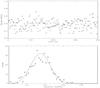 |
Fig. 1 Top: raw V2 measurements as a function of time for the calibrator on the night of Nov. 17th, 2009 at UT 12:17. Bottom: histogram of the V2 values of the previous sample. A Gaussian fit is superimposed on the data points. |
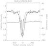 |
Fig. 2 Example of the differential visibility measurement obtained on ε Aur in high spectral resolution mode around the Hα line. The left vertical scale is for the relative intensity of the line profile (thin curve) and for the differential visibility amplitude relative to continuum (thick curve close to 1 at the minimum and maximum radial velocity). A Gaussian function (dashed curve) is fitted to the differential visibility amplitude. The right vertical scale corresponds to the differential phase measurements in degree (thick curve close to 0 at the minimum and maximum radial velocity). |
2.3. Obtaining the differential quantities
For the differential measurements in the high spectral resolution mode, we do not consider observations of calibrators before and after the science target. These data are instead dedicated to differential measurements through the spectral lines. The principle is described in Mourard et al. (2009). Firstly, we calculate the cross-spectrum between a large reference window and a narrow sliding science channel. Secondly, the raw differential measurements are corrected by removing the effect of the residual optical path difference and normalized to 1.0 in the continuum. An example of measurement is shown in Fig. 2. For the final science analysis, the amplitude of the differential visibility in the continuum is set to the value of the visibility in the reference channel, as calculated in Sect. 3. A Gaussian function is fitted to the differential visibility amplitude. This gaussian function is used to extract the minimum value of the visibility and the associated radial velocity and to estimate the full width at half maximum (in radial velocity) of the visibility drop. All the differential phase measurements have been oriented in the same way, which means that a positive offset represents an astrometric displacement towards the south in our case (Bonneau et al. 2011a; Meilland et al. 2011). The uncertainties of the differential interferometric quantities are obtained from a pure photon noise analysis. A more correct estimation is usually done through the dispersion of measurements in the continuum part of the data. The analysis we will present in Sect. 4 will lead to the estimation of global parameters of the Hα region for which error bars correctly account for the dispersion of measurements.
An accurate spectral calibration is mandatory for high spectral resolution interferometric analysis, but it must be admitted that, at present, the wavelength calibration of VEGA, based on a ThAr comparison spectrum, is not ideal. Part of the problem is that the limited wavelength interval used contains only a small number of suitable comparison lines. There can also be a problem of an occasional slight defocusing of the camera. To cope with this, we proceeded in the following way: we imported all VEGA Hα spectra into the program SPEFO (Horn et al. 1996; Škoda 1996), which was later improved by the late Mr. J. Krpata. Each rectified VEGA spectrum reduced to the heliocentric wavelength scale was then compared to the Ondřejov and/or Dominion Astrophysical Observatory red spectra already used by Chadima et al. (2011) or more recent ones, to be studied and published in detail by Harmanec et al. (in prep.), which were taken on roughly the same dates as the VEGA spectrum in question. A shift of the zero point of the wavelength scale was measured in this way and subsequently corrected in the VEGA spectra. This way, we also detected and corrected a few cases, when the original dispersion formula was not derived correctly. Some of the corrections of the zero point were not negligible, their total range being ±45 km s-1.
The differential measurements obtained on Hα are presented in Figs. A.1–A.3. Figures A.4–A.6 present the measurements for the Si lines, Fig. A.7 for the KI line and Fig. A.8 for the Na doublet.
3. Results from the continuum visibility measurements
In Table 1, we present the observations of ε Aur made in medium spectral resolution for the determination of calibrated squared visibilities. In the first step, we decided to derive a uniform disk equivalent diameter for each individual measurement. This is obviously a very rough approximation but it does illustrate that the object seen in the continuum is not symmetric at all and that this asymmetry has been changing from 2009 over 2010 to 2011. The results are presented in Table 1.
In Fig. 3, we present the results for the three main epochs of observation (November 2009, October 2010 and October 2011). It is interesting to note that whereas the out of eclipse observations of October 2011 do not exhibit strong changes with the position angle and a mean angular diameter of almost 2.1 mas, the observations of 2010 and 2009 show strong changes with the position angle of measurements and a clearly reduced size in 2010. This is undoubtedly a sign of a non-symmetric source in favor of the eclipsing body being a dark and sharp-edged, not a partly transparent object.
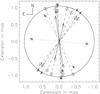 |
Fig. 3 The uniform disk equivalent angular diameter as a function of time (* and dotted line = november 2009, △ and solid line = october 2010, Λ and dashed line = october 2011). The axis are labeled in mas. The data are presented along the position angle of the baseline at the time of observation. The size of the small segments correspond to the uncertainty. The circle corresponds to an angular diameter of 2.1 mas. |
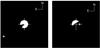 |
Fig. 4 Representation of the best solutions obtained for the 2009 (left) and 2010 (right) visibility measurements, assuming a model of ellipse for the eclipsing body according to K10. The centre of the ellipse is shown as a solid cross whereas the dotted one corresponds to the centre of the F star. The boxes are 12 mas on each side. |
As illustrated in Fig. 3, the uniform circular-disk approximation suggests significant differences in the apparent shape of the F star between 2009 and 2011. We use the CHARA+MIRC near-infrared continuum imaging obtained during this period (Kloppenborg et al. 2011) to guide the interpretation. We first used all the 2011 data together for a uniform disk estimate using the LitPro3 software (Tallon-Bosc et al. 2008). The result is θUD−660 nm = 2.10 ± 0.02 mas or θLD = 2.20 ± 0.02 mas. As seen in Fig. 3, the 2011 data show scatter and asymmetries are certainly expected. Recent MIRC 2011 imaging shows evidence for surface structures (Kloppenborg et al., in prep.). Thus, our value of the limb-darkening diameter should be taken as a rough estimate of the F star properties. For comparison, K10 obtained θUD−H = 2.10 ± 0.04 mas and Stencel et al. (2008) got θUD−K = 2.27 ± 0.11 mas.
We then adopted the ellipse model for the occulting disk as proposed by K10 (semimajor axis fixed to 6.1 mas and position angle to 120°, semiminor axis fixed to 0.61 mas) to check how they agree with our observations. We decided to constrain the position of the elliptical eclipsing body only. If the 2010 squared visibilities of Table 1 are used the best model gives a position of 0.9 mas to the west for the centre of the ellipse (mid-epoch November 2010). The 2009 data (mid-epoch November 2009) are also consistent with the ellipse model having a position of 5.2 mas to the east and 3.1 mas to the south. The best models are presented in Fig. 4. These values correspond to a motion of the eclipsing disk during almost one year for almost 7 mas from southeast to northwest with a position angle of 120°. The reduced χ2 of the best models are 0.5 for the 2009 data and 0.1 for 2010 (only two measurements). This result is a good confirmation of the conclusions obtained with the MIRC measurements and validates our squared visibility measurements. As we will see in the next section, this part of the analysis is very important in order to correctly set the level of differential visibilities in the spectrally resolved measurements.
4. Analysis of the spectral line differential measurements
The rotation sense of the disk is well established as redshifted during ingress and blueshifted during egress (Chadima et al. 2011). Moreover, this angular momentum vector is parallel to the observed orbital motion of the disk around the system center of mass (Kloppenborg et al. 2010). Thus, we can assume that the F star rotation axis is parallel to these, and consistent with its own orbital motion (Chadima et al. 2011; Stefanik et al. 2010).
4.1. Qualitative behavior of the differential visibilities
The intensity (ℐ), visibility ( ) and phase shift (
 ) of the profiles in Hα are displayed in Figs. A.1–A.3. As we are considering differential quantities for the interferometric measurements, the visibility accounts for the relative size of the region of interest at a certain wavelength with respect to the size of the object in the continuum. We note that during 2009, when the redshifted portions of the rotating disk were beginning to occult the blueshifted side of the F star, three of four profiles show
  1 for λ < λo, with λo the central wavelength of the line, suggesting that photons from the F star are being scattered by extended hydrogen associated with disk material – which mainly covers the blueshifted hemisphere of the F star during ingress (2009). Phase shifts in three of the four spectra are positive, implying a source offset (Bonneau et al. 2011a; Meilland et al. 2011) to the south of the F star photocentre, which is consistent with the disk’s orbital plane offset as defined by the interferometric imaging.
The visibility in the Si II line (Figs. A.4–A.6) shows some differential signal with respect to the continuum during 2009, but the amplitudes are minimal, with a small amount of blueshift relative to the line core. The very weak K I 769.9 nm lines (Fig. A.7) show virtually no visibility change or phase shifts at any epoch.
During 2010, the full-eclipse phase, the intensity profile broadens, where ~ 1 at all wavelengths. This indicates that both red- and blue-shifted line-of-sight components are involved, as expected during the central eclipse (August). After August 2010 (RJD > 55 450), as far as the signal-to-noise ratio of the data allows, we see, in the S-shape of the differential phase, a signature of disk rotation in the development of a blue-shifted excess in the intensity profile. During this time, the visibility minimum remains closer to the rest wavelength, indicating that the line of sight contains hydrogen in a region that extends perpendicularly to the plane of the disk, as seen during the conjunction. Positive phase shifts are seen in half of the higher signal-to-noise spectra, with strong phase shifts seen on 27 Aug. (RJD = 55 436) and 11 Oct. (RJD = 55 480), again consistent with the disk occulting the southern part of the F star photosphere.
During 2010, the Si II lines show variable visibilities but the difficulties in correctly calibrating the neighboring continuum prevent us for a more quantitative analysis. The much stronger Na D lines (Fig. A.8) show a different visibility signal on the blue side of the line intensity profiles, consistent with the blue-shifted portions of the disk being in the line of sight at those epochs, although less resolved than in Hα.
During 2011, after the photometric eclipse ended, the spectroscopic one still continued in strong spectral lines. This indicated that the blue-shifted material coming from the extended disk atmosphere was still present in the line of sight to the F star. We also see that  for λ > λo, indicating that the blue-shifted disk material and/or material toward the red-shifted limb of the F star is more resolved, and hence larger than the F star photosphere. The magnitude of this effect seems to diminish over the 2011 autumn interval monitored, although the wing emission could be a factor affecting this. Positive phase shifts are seen again in half of the spectra. Even though the optically thick portion of the disk has passed, there is lagging material still affecting the Hα intensity profile and the phase shifts, consistent with the offset toward the southern half of the F star photosphere.
Also during 2011, the Si II lines continue to behave as previously noted, except with possibly stronger evidence for blue-shift relative to intensity centre (20 Sept., RJD = 55 825). The single Na D observation is consistent with those seen in 2010 but with larger phase shifts.
4.2. Quantitative analysis of the Hα measurements
In order to compare all the Hα differential visibility measurements, and lacking a detailed toy-model with time dependence (which is out of the scope of this paper), we first fit a Gaussian function to the visibility modulus. Although some of the differential visibility curves exhibit some bimodal behavior or some asymmetry, the choice of this representation is really helpful for a global description of the measurements. This permits us to extract the minimum value of the visibility and to estimate the full width at half maximum (in radial velocity) of the visibility drop as well as the velocity shift as a function of time. The mean value of the reduced χ2 for all the 22 measurements is 2.3. Results are given in Table 5.
VEGA observations of ϵ Aurigae in high resolution mode around Hα.
First we estimate the size in mas of the Hα absorbing region considered as Gaussian. The computation of the differential visibility amplitude (Mourard et al. 2009) gives, as result, the product of the visibility amplitude in the continuum (the reference channel) by the value of the visibility amplitude in the science channel. We use the ellipse model developed in Sect. 3 to estimate the visibility amplitude in the continuum at each date and projected baseline and then obtain the final estimate of the calibrated visibility amplitude in the core of the Hα spectral line. The size is thereby estimated, taking into account the projected baseline at the time of the observations and a Gaussian model. Results are presented in Fig. 5-left. The interpretation is discussed in Sect. 5.
Although the 2009 data are highly dispersed (note that no external fringe tracking was available at that time), we notice a tendency for the annual average Hα size to increase as a function of time. It’s clear, however, that even at the beginning of the eclipse, the Hα region has extended to twice the size of the F star. From the Gaussian fit of the visibility drop, we can also estimate the range of velocities (FWHM and central velocity) affected by the Hα visibility decrease. The results are presented in Fig. 5.
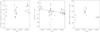 |
Fig. 5 In Figs A.1–A.3, we fit a Gaussian curve for the visibility drop in the Hα line. The left panel presents, as a function of the reduced heliocentric Julian date, the size in mas of the Hα region deduced from the minimum of visibility and modeled as a Gaussian function. In the middle panel we show the evolution of the velocity shift for the minimum of visibility (△ ) overplotted with the radial velocity determined by spectroscopy directly (+ signs). The solid line represents the radial velocity of the F star orbital motion. In the right panel, the width in velocity of the visibility drop is displayed. In all 3 panels, the horizontal scale is the reduced heliocentric Julian date. |
4.3. Astrometric position of the Hα core
Measuring differential phases allows us to locate the position of the photocentre of the emitting source as a function of wavelength, or at least the projection of this position along the direction of the projected baseline. As the observations were only possible with the S1S2 baseline, oriented mainly south-north, we dedicated some nights to obtain at least two projections at two different position angles as detailed in Table 2. However, in certain cases, the quality in the differential phase measurements was not sufficient to allow a reliable determination of the position of the photocentre. After the final data analysis, we obtained the correct positions for two dates in Nov. 2009, two in Oct. 2010, and two in Oct. 2011 (see Table 6 and Fig. 6).
Position (in mas) of the photocentre of the resolved Hα region deduced from the projection along the baseline direction.
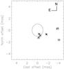 |
Fig. 6 Representation of the photocentre position of the Hα region as determined from differential phase measurements. * Symbol (respectively △ and Λ) corresponds to 2009 (resp. 2010 and 2011). The circle represents the disk of the F star. |
These measurements clearly demonstrate that the region responsible for the core of the Hα absorption is south shifted with respect to the photocentre of the F star. In addition to the global astrometric shift, another interesting feature seen in the differential phases is the S-shape signal observed at certain phases in 2009 and 2011. This S-shape signal in phase is classically interpreted as the signature of a rotational velocity field.
5. Discussion
5.1. Behavior of the Hα region
As primary results of the VEGA/CHARA interferometric analysis in the Hα line, we have obtained three main interesting results.
As seen in the middle panel of Fig. 5, the wavelength shift in the Gaussian-fitted FWHM of the visibility in Hα follows the F star orbital motion, except during total eclipse in 2010, where it resembles the sign and amplitude of disk rotation as determined in other spectral lines (Lambert & Sawyer 1986). The solid line in the middle panel is the theoretical RV curve based on the PHOEBE solution by Chadima et al. (2010).
As seen in the right panel of Fig. 5, the Gaussian-fitted Hα visibility drop width varies between 95–116 ± 13 km s-1FWHM during early eclipse phases (2009) and post-eclipse (2011) but the average increased to 148 ± 18 km s-1 during eclipse phase (2010).
Early in-eclipse (2009, Fig. A.1) and again post-eclipse (2011, Fig. A.3), the visibility is reduced (and the object is therefore more resolved) in the Hα line wings, often on the blue side of the line core, where emission is present in the intensity spectrum. This visibility decrease can be explained by the addition of an extended component, or by the decrease of the flux from the compact source (i.e., the F supergiant) by some absorption. Such a phenomenon is observed in the blue part of P Cygni-type lines observed in stars exhibiting strong winds. Therefore the observed differential visibility is a complex integral of emission and absorption from the line, that can itself be distributed in several detached components. The effect on visibilities due to P Cygni outflows is discussed by ten Brummelaar et al. (2011) and Tallon-Bosc et al. (in prep.).
With this in hand, we can use the VEGA/CHARA observations, along with prior information, to test a three component model: (a) the 2.1 mas diameter F star, rotating eastward at ~40 km s-1, with its north pole position angle at ~30 degrees; (b) the horizontally and vertically extended disk that creates the eclipse, also rotating eastward at ~30 km s-1 and presenting line-of-sight components that are mainly red-shifted in 2009, and mainly blue-shifted thereafter; and (c) a nebular region associated with the F star, which we hypothesize extends toward the direction of the disk. The interferometric observations demonstrate that the optically thick disk moves to the west across the face of the F star, occulting the southern hemisphere.
5.2. Evidences for a stellar wind
We also re-investigated the RV curves of the red Si II and Fe II lines published by Chadima et al. (2011) and the RV curve of the whole Hα emission derived by Harmanec et al. (in prep.) from a comparison of individual Hα line profiles with the mean out-of-eclipse one. Using the program FOTEL (Hadrava 1990, 2004), we only allowed for calculation of the semi-amplitude K1 and systemic velocity γ, keeping all other orbital elements fixed at the values derived by Chadima et al. (2010) in PHOEBE. We obtained the following results: 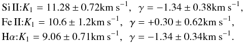 \arraycolsep1.75ptThis seems to indicate that the bulk of the Hα emission moves mostly within the orbit of the F star, though the marginally significant lower amplitude of the Hα RV curve in comparison to the metallic lines could indicate that the optical centre of gravity of the Hα emission is a bit closer to the centre of gravity of the binary than the mass centre of the F star. It may show that there is more emissivity on the side facing the dark disk (filling the “nose”, reminiscent of the critical Roche lobe of circular orbits).
The VEGA/CHARA visibilities are suggestive of a P Cygni-like expansion of the F star hemisphere facing earth and the disk during eclipse phases. We also have evidence for similar outflows seen in ultraviolet spectra. HST+COS data were obtained during 2010 autumn (Howell et al. 2011) where several doubly-reversed lines were seen, including the C II 133.5 nm doublet that shows a clear set of P Cygni profiles with an absorption component displaced by −68 km s-1 relative to the emission component. The same profiles at lower resolution were illustrated by Sheffer & Lambert (1999) in data obtained in 1996 at a phase opposite to the primary eclipse, but these were not discussed in their paper. The increase in the VEGA visibility FWHM during maximum eclipse (2010) indicates additional forward scattering due to the introduction of material surrounding the disk, essentially an atmosphere dominated by hydrogen, but capable of more fully eclipsing the F star than the semi-eclipse caused by the denser portion of the disk imaged at near-IR wavelengths by CHARA+MIRC (Kloppenborg et al. 2011). Future observations with VEGA/CHARA will permit analysis of the part of the disk facing the F star in order to improve our understanding of the wind forming mechanism.
5.3. Constraints on the mass of the central object in the disk
As discussed in Sect. 3, our VEGA+CHARA observations strongly suggest that the hydrogen gas fully eclipses the F star and is at least twice the near-IR value (2.4 mas).
For strictly thermal dispersion of material, the scale height H to disk radius RD ratio equals the sound-speed-to-Keplerian velocity ratio, which is: 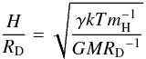 (2)(Lissauer et al. 1996), where mH is the mass of a hydrogen atom, M the mass of the disk and γ is the ratio of specific heats (5/3 for ideal gases). The observed ratio of the measured thickness of the gas disk (2.1 mas) relative to the disk radius (6.10 mas), is 0.34. Figures and tables included in Lissauer et al. (1996) indicate that the disk thickness is of order two to three times the scale height, implying the scale height to disk radius falls in the range 0.11 to 0.17. Given an observed range of disk temperatures, 550 K to 1100 K (Stencel et al. 2011), the hydrogen gas thermal speed is 2.8 to 3.9 km s-1. Given this and the scale height to disk radius ratio, 0.11 to 0.17, we deduce the quantity (GM/R)0.5 to be 23 to 35 km s-1, which implies the central mass to be in the range, M2 = 2.4−5.6 M⊙. For comparison, translating the above values to absolute dimensions requires a knowledge of the distance to ε Aur. Adopting the nominal Hipparcos distance, d = 650 pc, one obtains the disk radius of 3.97 AU. Using these values and Keplerian rotation, this implies the mass of the star hidden in the disk to be M2 = 2.4−5.5 M⊙. Using the distance of 1050 pc (advocated by Johnston et al. 2012), one gets a disk radius of 6.41 AU and M2 = 3.8−9.1 M⊙.
The activity associated with the F star is explained in this picture, a “focused wind” (Friend & Castor 1982) directed from the F star toward the inner Lagrangian point in the system, some of the stellar wind mass can be expected to be transferred to the disk. This Roche region should become increasingly apparent to interferometric imaging as the system approaches quadrature and should be monitored. de Jager et al. (1988) compiled mass loss rate estimates for other yellow supergiants, and these are in the range of 10-8 M⊙ yr-1. If only one percent of the outflow is captured, that provides 10-10 M⊙ yr-1 input to the disk, or about 10-4 of its estimated mass, sufficient to sustain the disk against accretion for aeons.
6. Conclusion
Thanks to high angular and spectral resolution measurements of ε Aur obtained with the VEGA instrument on the CHARA optical array from 2009 to 2011, we have been able to reveal some of the features of the gaseous disk surrounding the unseen companion responsible of the eclipse. Hα originates in an expanding zone almost twice the photospheric size of the F star and extending above and below the plane of the disk itself. With additional assumptions, we deduce some mass constraints for the central object inside the eclipsing disk.
Post-eclipse observations in the coming seasons will permit detailed study of the part of the disk facing the F star, enabling us to understand the origin of the mechanism of stellar wind that we saw.
Online material
Appendix A: Overview of spectrointerferometric observations
Here, we present detailed plots of the spectra, differential visibilities and differential phases for the Hα, Si II, Na I and K I lines. In all cases, the differential phases measurements have been oriented in the same way, which means that a positive offset corresponds to an astrometric displacement towards the south.
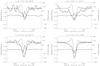 |
Fig. A.1 Hα 2009: spectrum, differential visibility and differential phase. The left vertical scale is the relative intensity of the line profile (thin curve) and the differential visibility amplitude relative to continuum (thick curve close to 1 at the minimum and maximum radial velocity). A Gaussian function (dotted curve) is fitted to the differential visibility amplitude. It permits the extraction of the line and visibility measurements. The right vertical scale corresponds to the differential phase measurements in degree (thick curve close to 0 at the minimum and maximum radial velocity). |
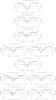 |
Fig. A.2 Hα 2010: spectrum, differential visibility and differential phase. See Fig. A.1 for axis and plot explanations. |
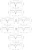 |
Fig. A.3 Hα 2011: spectrum, differential visibility and differential phase. See Fig. A.1 for axis and plot explanations. |
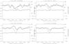 |
Fig. A.4 SiII 2009: spectrum, differential visibility and differential phase. The left vertical scale is the relative intensity of the line profile (thin curve) and the differential visibility amplitude relative to continuum (thick curve close to 1 at the minimum and maximum radial velocity). The right vertical scale corresponds to the differential phase measurements in degree (thick curve close to 0 at the minimum and maximum radial velocity). |
 |
Fig. A.5 SiII 2010: spectrum, differential visibility and differential phase. See Fig. A.4 for axis and plot explanations. |
 |
Fig. A.6 SiII 2011: spectrum, differential visibility and differential phase. See Fig. A.4 for axis and plot explanations. |
 |
Fig. A.7 KI: spectrum, differential visibility and differential phase. The left vertical scale is the relative intensity of the line profile (thin curve) and the differential visibility amplitude relative to continuum (thick curve close to 1 at the minimum and maximum radial velocity). The right vertical scale corresponds to the differential phase measurements in degree (thick curve close to 0 at the minimum and maximum radial velocity). |
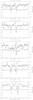 |
Fig. A.8 NaD: spectrum, differential visibility and differential phase. See Fig. A.7 for axis and plot explanations. |
See, e.g., http://www.hposoft.com/EAur09/Spectroscopy.html or Harmanec et al. (in prep.).
The software application is available at http://www.jmmc.fr/searchcal
Available at http://www.jmmc.fr/litpro
Acknowledgments
The CHARA Array is operated with support from the National Science Foundation through grant AST-0908253, the W. M. Keck Foundation, the NASA Exoplanet Science Institute, and from Georgia State University. D.M. warmly thanks all the VEGA observers that permitted the acquisition of this set of data. We profited from the use of the program SPEFO, written by our late colleague Dr. Jiří Horn and program FOTEL written by Dr. P. Hadrava. The research of P.H. was supported by the grant P209/10/0715 of the Czech Science Foundation and also from the Research Program MSM0021620860 Physical study of objects and processes in the solar system and in astrophysics of the Ministry of Education of the Czech Republic. We acknowledge the use of the electronic database from the CDS, Strasbourg and electronic bibliography maintained by the NASA/ADS system. This work also was supported in part by the bequest of William Herschel Womble in support of astronomy at the University of Denver, and by NSF grant AST 10-16678 to the University of Denver.
References
- Bonneau, D., Clausse, J.-M., Delfosse, X., et al. 2006, A&A, 456, 789 [NASA ADS] [CrossRef] [EDP Sciences] [Google Scholar]
- Bonneau, D., Chesneau, O., Mourard, D., et al. 2011a, A&A, 532, A148 [NASA ADS] [CrossRef] [EDP Sciences] [Google Scholar]
- Bonneau, D., Delfosse, X., Mourard, D., et al. 2011b, A&A, 535, A53 [NASA ADS] [CrossRef] [EDP Sciences] [Google Scholar]
- Carroll, S. M., Guinan, E. F., McCook, G. P., & Donahue, R. A. 1991, ApJ, 367, 278 [NASA ADS] [CrossRef] [Google Scholar]
- Cha, G., Tan, H., Xu, J., & Li, Y. 1994, A&A, 284, 874 [NASA ADS] [Google Scholar]
- Chadima, P., Harmanec, P., Yang, S., et al. 2010, IBVS, 5937, 1 [NASA ADS] [Google Scholar]
- Chadima, P., Harmanec, P., Bennett, P. D., et al. 2011, A&A, 530, A146 [NASA ADS] [CrossRef] [EDP Sciences] [Google Scholar]
- de Jager, C., Nieuwenhuijzen, H., & van der Hucht, K. A. 1988, A&AS, 72, 259 [NASA ADS] [Google Scholar]
- Eggleton, P. P., & Pringle, J. E. 1985, ApJ, 288, 275 [NASA ADS] [CrossRef] [Google Scholar]
- Friend, D. B., & Castor, J. I. 1982, ApJ, 261, 293 [NASA ADS] [CrossRef] [Google Scholar]
- Hadrava, P. 1990, Contributions of the Astronomical Observatory Skalnaté Pleso, 20, 23 [Google Scholar]
- Hadrava, P. 2004, Publ. Astron. Inst. Acad. Sci. Czech Rep., 92, 1 [Google Scholar]
- Hoard, D. W., Howell, S. B., & Stencel, R. E. 2010, ApJ, 714, 549 [Google Scholar]
- Hoffleit, D., & Jaschek, C. 1982, The Bright Star Catalogue (Yale University Observatory) [Google Scholar]
- Hoffleit, D., Saladyga, M., & Wlasuk, P. 1983, Bright star catalogue, Supplement (Yale University Observatory) [Google Scholar]
- Hopkins, J., & Stencel, R. E. 2004, in BAAS, 36, 107.05 [Google Scholar]
- Horn, J., Kubát, J., Harmanec, P., et al. 1996, A&A, 309, 521 [NASA ADS] [Google Scholar]
- Howell, S. B., Stencel, R. E., & Hoard, D. W. 2011, in BAAS, 43, 257.07 [Google Scholar]
- Johnston, C., Guinan, E., Harmanec, P., & Mayer, P. 2012, in BAAS, 44, 153.34 [Google Scholar]
- Kim, H. 2008, J. Astron. Space Sci., 25, 1 [NASA ADS] [CrossRef] [Google Scholar]
- Kloppenborg, B., Stencel, R., Monnier, J. D., et al. 2010, Nature, 464, 870 [NASA ADS] [CrossRef] [PubMed] [Google Scholar]
- Kloppenborg, B. K., Stencel, R., Monnier, J. D., et al. 2011, in BAAS, 43, 257.03 [Google Scholar]
- Kuiper, G. P., Struve, O., & Strömgren, B. 1937, ApJ, 86, 570 [NASA ADS] [CrossRef] [Google Scholar]
- Lambert, D. L., & Sawyer, S. R. 1986, PASP, 98, 389 [NASA ADS] [CrossRef] [Google Scholar]
- Leadbeater, R., & Stencel, R. 2010 [arXiv:1003.3617] [Google Scholar]
- Lissauer, J. J., Wolk, S. J., Griffith, C. A., & Backman, D. E. 1996, ApJ, 465, 371 [NASA ADS] [CrossRef] [Google Scholar]
- Ludendorff, H. 1903, AN, 164, 81 [NASA ADS] [CrossRef] [Google Scholar]
- Meilland, A., Delaa, O., Stee, P., et al. 2011, A&A, 532, A80 [NASA ADS] [CrossRef] [EDP Sciences] [Google Scholar]
- Mourard, D., Clausse, J. M., Marcotto, A., et al. 2009, A&A, 508, 1073 [NASA ADS] [CrossRef] [EDP Sciences] [Google Scholar]
- Sheffer, Y., & Lambert, D. L. 1999, PASP, 111, 829 [NASA ADS] [CrossRef] [Google Scholar]
- Škoda, P. 1996, in Astronomical Data Analysis Software and Systems V, eds. G. H. Jacoby, & J. Barnes, ASP Conf. Ser., 101, 187 [Google Scholar]
- Stefanik, R. P., Torres, G., Lovegrove, J., et al. 2010, AJ, 139, 1254 [NASA ADS] [CrossRef] [Google Scholar]
- Stencel, R. E., Creech-Eakman, M., Hart, A., et al. 2008, ApJ, 689, L137 [NASA ADS] [CrossRef] [Google Scholar]
- Stencel, R. E., Kloppenborg, B. K., Wall, Jr., R. E., et al. 2011, AJ, 142, 174 [NASA ADS] [CrossRef] [Google Scholar]
- Struve, O. 1956, PASP, 68, 27 [NASA ADS] [CrossRef] [Google Scholar]
- Sturmann, J., Ten Brummelaar, T., Sturmann, L., & McAlister, H. A. 2010, in Proc. SPIE, 7734 [Google Scholar]
- Tallon-Bosc, I., Tallon, M., Thiébaut, E., et al. 2008, in Proc. SPIE, 7013 [Google Scholar]
- ten Brummelaar, T. A., Huber, D., von Braun, K., et al. 2011 [arXiv:1107.2890] [Google Scholar]
- van Leeuwen, F. 2007a, Hipparcos, the New Reduction of the Raw Data (Berlin: Springer), Astrophys. Space Sci. Lib., 350 [Google Scholar]
- van Leeuwen, F. 2007b, A&A, 474, 653 [NASA ADS] [CrossRef] [EDP Sciences] [Google Scholar]
- Welty, D. E., & Hobbs, L. M. 2001, ApJS, 133, 345 [NASA ADS] [CrossRef] [Google Scholar]
- Zorec, J., Cidale, L., Arias, M. L., et al. 2009, A&A, 501, 297 [NASA ADS] [CrossRef] [EDP Sciences] [Google Scholar]
All Tables
VEGA observations of ε Aur in medium resolution for squared visibility measurement in the continuum near Hα.
VEGA observations of ε Aur in high resolution mode in Hα and Si II 634.7 nm lines.
Position (in mas) of the photocentre of the resolved Hα region deduced from the projection along the baseline direction.
All Figures
|
Fig. 1 Top: raw V2 measurements as a function of time for the calibrator on the night of Nov. 17th, 2009 at UT 12:17. Bottom: histogram of the V2 values of the previous sample. A Gaussian fit is superimposed on the data points. |
| In the text | |
|
Fig. 2 Example of the differential visibility measurement obtained on ε Aur in high spectral resolution mode around the Hα line. The left vertical scale is for the relative intensity of the line profile (thin curve) and for the differential visibility amplitude relative to continuum (thick curve close to 1 at the minimum and maximum radial velocity). A Gaussian function (dashed curve) is fitted to the differential visibility amplitude. The right vertical scale corresponds to the differential phase measurements in degree (thick curve close to 0 at the minimum and maximum radial velocity). |
| In the text | |
|
Fig. 3 The uniform disk equivalent angular diameter as a function of time (* and dotted line = november 2009, △ and solid line = october 2010, Λ and dashed line = october 2011). The axis are labeled in mas. The data are presented along the position angle of the baseline at the time of observation. The size of the small segments correspond to the uncertainty. The circle corresponds to an angular diameter of 2.1 mas. |
| In the text | |
|
Fig. 4 Representation of the best solutions obtained for the 2009 (left) and 2010 (right) visibility measurements, assuming a model of ellipse for the eclipsing body according to K10. The centre of the ellipse is shown as a solid cross whereas the dotted one corresponds to the centre of the F star. The boxes are 12 mas on each side. |
| In the text | |
|
Fig. 5 In Figs A.1–A.3, we fit a Gaussian curve for the visibility drop in the Hα line. The left panel presents, as a function of the reduced heliocentric Julian date, the size in mas of the Hα region deduced from the minimum of visibility and modeled as a Gaussian function. In the middle panel we show the evolution of the velocity shift for the minimum of visibility (△ ) overplotted with the radial velocity determined by spectroscopy directly (+ signs). The solid line represents the radial velocity of the F star orbital motion. In the right panel, the width in velocity of the visibility drop is displayed. In all 3 panels, the horizontal scale is the reduced heliocentric Julian date. |
| In the text | |
|
Fig. 6 Representation of the photocentre position of the Hα region as determined from differential phase measurements. * Symbol (respectively △ and Λ) corresponds to 2009 (resp. 2010 and 2011). The circle represents the disk of the F star. |
| In the text | |
|
Fig. A.1 Hα 2009: spectrum, differential visibility and differential phase. The left vertical scale is the relative intensity of the line profile (thin curve) and the differential visibility amplitude relative to continuum (thick curve close to 1 at the minimum and maximum radial velocity). A Gaussian function (dotted curve) is fitted to the differential visibility amplitude. It permits the extraction of the line and visibility measurements. The right vertical scale corresponds to the differential phase measurements in degree (thick curve close to 0 at the minimum and maximum radial velocity). |
| In the text | |
|
Fig. A.2 Hα 2010: spectrum, differential visibility and differential phase. See Fig. A.1 for axis and plot explanations. |
| In the text | |
|
Fig. A.3 Hα 2011: spectrum, differential visibility and differential phase. See Fig. A.1 for axis and plot explanations. |
| In the text | |
|
Fig. A.4 SiII 2009: spectrum, differential visibility and differential phase. The left vertical scale is the relative intensity of the line profile (thin curve) and the differential visibility amplitude relative to continuum (thick curve close to 1 at the minimum and maximum radial velocity). The right vertical scale corresponds to the differential phase measurements in degree (thick curve close to 0 at the minimum and maximum radial velocity). |
| In the text | |
|
Fig. A.5 SiII 2010: spectrum, differential visibility and differential phase. See Fig. A.4 for axis and plot explanations. |
| In the text | |
|
Fig. A.6 SiII 2011: spectrum, differential visibility and differential phase. See Fig. A.4 for axis and plot explanations. |
| In the text | |
|
Fig. A.7 KI: spectrum, differential visibility and differential phase. The left vertical scale is the relative intensity of the line profile (thin curve) and the differential visibility amplitude relative to continuum (thick curve close to 1 at the minimum and maximum radial velocity). The right vertical scale corresponds to the differential phase measurements in degree (thick curve close to 0 at the minimum and maximum radial velocity). |
| In the text | |
|
Fig. A.8 NaD: spectrum, differential visibility and differential phase. See Fig. A.7 for axis and plot explanations. |
| In the text | |
Current usage metrics show cumulative count of Article Views (full-text article views including HTML views, PDF and ePub downloads, according to the available data) and Abstracts Views on Vision4Press platform.
Data correspond to usage on the plateform after 2015. The current usage metrics is available 48-96 hours after online publication and is updated daily on week days.
Initial download of the metrics may take a while.